The MHD equation of state with post-Holtsmark microfield distributions

Abstract

The Mihalas-Hummer-Däppen (MHD) equation of state is a part of the Opacity Project (OP), where it mainly provides ionization equilibria and level populations of a large number of astrophysically relevant species. Its basic concept is the idea of perturbed atomic and ionic states. At high densities, when many-body effects become dominant, the concept of perturbed atoms loses its sense. For that reason, the MHD equation of state was originally restricted to the plasma of stellar envelopes, that is, to relatively moderate densities, which should not exceed $\rho<10^{-2}$ g cm^-3. However, helioseismological analysis has demonstrated that this restriction is much too conservative. The principal feature of the original Hummer & Mihalas (1988) paper is an expression for the destruction probability of a bound state (ground state or excited) of a species (atomic or ionic), linked to the mean electric microfield of the plasma. Hummer & Mihalas (1988) assumed, for convenience, a simplified form of the Holtsmark microfield for randomly distributed ions. An improved MHD equation of state (Q-MHD) is introduced. It is based on a more realistic microfield distribution (Hooper 1966, 1968) that includes plasma correlations. Comparison with an alternative post-Holtsmark formalism (APEX) is made, and good agreement is shown. There is a clear signature of the choice of the microfield distribution in the adiabatic index $\gamma_{1}$, which makes it accessible to present-day helioseismological analysis. But since these thermodynamic effects of the microfield distribution are quite small, it also follows that the approximations chosen in the original MHD equation of state were reasonable. A particular feature of the original MHD papers was an explicit list of the adopted free energy and its first- and second-order analytical derivatives. The corresponding Q-MHD quantities are given in the Appendix.

1 Introduction

The so-called MHD equation of state (Hummer & Mihalas 1988; Mihalas et al. (1988); Däppen et al. (1988); Däppen et al. (1987)) was developed as part of the international “Opacity Project” (OP; see Seaton 1987, 1992, (1995); Berrington (1997)). Its main purpose was to calculate the ionization degrees of all astrophysically relevant chemical elements in order to provide a crucial ingredient of the calculation of the radiative opacity of stellar interiors. The basic concept of the MHD equation of state was built on the idea of perturbed atomic and ionic states. At high densities, when many-body effects become dominant, the concept of perturbed atoms loses its sense. For that reason, the MHD equation of state was originally restricted to the plasma of stellar envelopes, that is, to relatively moderate densities, which should not exceed $\rho<10^{-2}$ g cm^-3.

However, the MHD calculation of ionization equilibria was not only the necessary part of an opacity calculation. The same analytical and computational effort also allowed the computation of thermodynamic quantities to a high degree of accuracy and reliability. It turned out that for the purpose of thermodynamic calculations, the aforementioned density domain was much too conservative. For instance, Christensen-Dalsgaard et al. (1988) applied the MHD equation of state to models of the entire Sun in order to predict solar oscillation frequencies. MHD remained a reliable tool down to the solar center, where density is about 150 g cm^-3. So in spite of the original design of the MHD equation of state, the associated thermodynamic expressions have a broader domain of applicability, extending in particular to stellar cores. The reason is that in the deeper interior, the plasma becomes virtually fully ionized. Therefore, in practice, it does not matter that the condition for the legitimacy of the perturbation mechanism for bound species (Hummer & Mihalas 1988) is not fulfilled, essentially because there are no bound species of the chemical elements that can be relevant for the equation of state (however, for opacity, bound states of less abundant elements are relevant). Without bound species, the MHD equation of state falls back to an ideal-gas equation, enriched with Coulomb pressure and electron degeneracy. Coulomb pressure is only included to lowest order (the Debye-Hückel approximation, see, e.g., Ebeling et al. (1976)), yet it is now known that, somewhat fortuitously, the lack of higher-order Coulomb term has no significant consequence (for more details see Christensen-Dalsgaard et al. (1996)). Specifically, it was shown by Chabrier & Baraffe (1997) that the MHD equation of state can be used for low-mass stars, at least down to 0.4 M_⊙ (see also Trampedach & Däppen (1999)).

Helioseismology has so far been putting the toughest observational constraints on the equation of state (for a recent review, see Christensen-Dalsgaard et al. (1999)). Given the importance of helioseismology as an experiment, we specifically review some of the most recent results in Section 3. It has emerged that the MHD equation of state clearly fares well, especially in comparisons with simpler formalisms, for instance the popular Eggleton, Faulkner & Flannery (1973) equation of state (hereinafter EFF). However, there are still discrepancies between MHD and the inference from observations (Christensen-Dalsgaard et al. (1996)). Some of these discrepancies were successfully removed by the OPAL equation of state (which is itself part of a major opacity project; Rogers (1986); Iglesias & Rogers 1995; Rogers et al. (1996) and references therein). However, recent results by Basu et al. (1999) have indicated that in the outermost layers of the Sun ($r/R_{\odot}>0.97$), the MHD equation of state appears to be a better match to the data than OPAL (see Section 3).

The continual involvement of the MHD equation of state in current developments has led us to revisit the principal issues. The original Hummer & Mihalas (1988) paper derived an expression for the destruction probability of a bound state (ground state or excited) of a species (atomic or ionic). The probability was expressed as a function of the mean electric microfield. For convenience, Hummer & Mihalas (1988) assumed a Holtsmark microfield for randomly distributed ions. Furthermore, to reduce the computational effort, they adopted a simplified approximate form of the Holtsmark function.

It turned out that these simplifications have been the source of inadequacies of the MHD equation of state. In a real plasma, correlations occur, that is, the Coulomb interaction modifies the ion distribution. The result is that the microfield distribution peaks at lower values of the field strength than given by the Holtsmark distribution. Therefore, the probability with which a state for a specific atom or ion ceases to exist is reduced relative to the Holtsmark result, and thus finally, the occupation probabilities is higher than in the Holtsmark approximation. These discrepancies were demonstrated by Iglesias & Rogers (1995). Therefore, the poor quality of the Holtsmark approximation is one of the reasons for the discrepancy between OP and OPAL opacities at higher densities.

One might think that these differences would have only a small bearing on the equation of state (Rogers & Iglesias 1998). However, recent studies about the influence of details in the hydrogen partition function on thermodynamic quantities (Nayfonov & Däppen 1998; Basu et al. 1999) have revealed that the difference between various approximations of the microfield distribution is well within range of observational helioseismology (see Section 3). In view of these more stringent demands on the equation of state, we have improved the original MHD equation of state by including a post-Holtsmark microfield distribution to account for particle correlation. This microfield distribution function was derived by Hooper (1966, 1968). Here, we present the resulting improved MHD equation of state. We name it “Q-MHD” after Hummer ’s (1986) nomenclature (in which the microfield distribution was called P and its integral Q). Comparison with an alternative post-Holtsmark formalism (APEX; see Iglesias et al. (1985) and references therein) is made, and good agreement is shown. Since one of the main features of the original MHD papers was an explicit list of the free energy and its first- and second-order analytical derivatives, we list all the corresponding Q-MHD quantities in the Appendix.

2 The MHD Equation of State

The majority of the realistic equations of state that have appeared in the last 30 years are based on the so-called “free-energy minimization method”. Before that, a common method was to use one expression (e.g., a modified Saha equation) for the ionization equilibria and another (not necessarily consistent) expression for the thermodynamic quantities. Such a procedure can lead to violations of Maxwell relations. The prevention is of course the use of a single thermodynamic potential, e.g., the free energy. Then, thermodynamic consistency is built in. However, since such a method requires considerable computing power, especially for multi-component plasmas, it could only become feasible since about 1960 (Harris (1959); Harris et al. (1960)).

The free-energy minimization method uses statistical-mechanical models (for example, a partially degenerate electron gas, Debye-Hückel theory for ionic species, hard-sphere atoms to simulate pressure ionization via configurational terms, quantum mechanical models of atoms in perturbed fields, etc.). It is a modular approach, that is, these models become the building blocks of a macroscopic free energy, which is expressed as a function of temperature $T$, volume $V$, and the particle numbers $N_{1},\ldots,N_{m}$ of the $m$ components of the plasma. This model free energy is then minimized, subject to the stoichiometric constraints. The solution of this minimization problem then gives both the equilibrium concentrations and, if inserted in the free energy and its derivatives, the equation of state and the thermodynamic quantities. Obviously, this procedure automatically guarantees thermodynamic consistency. For obvious reason, this approach is called the “chemical picture”. Perturbed atoms must be introduced on a more or less ad-hoc basis to avoid the familiar divergence of internal partition functions (see, e.g., Ebeling et al. (1976)).

2.1 Internal Partition Functions

The simplest way to modify atomic or ionic bound states to account for effects of the surroundings is by truncating the internal partition function at some maximum level that can be a function of temperature and density. Such a modification of bound states runs into the well-known technical problem that whenever the density passes through a critical value, for which a given bound state disappears into the continuum, the partition function changes discontinuously by the amount of the statistical weight $g_{i}$ of the state. This is clearly unphysical and would lead to discontinuities and singularities in the free energy and its derivatives.

One way of avoiding the problem of discontinuous jumps in the partition function is to assign “weights” or “occupation probabilities” to all bound states of all species. The internal partition function then becomes

$$Z_{jk}^{\rm int}=\sum_{i}{w_{ijk}}~{}{g_{ijk}}{\exp\left[-E_{ijk}/(k_{\rm B}T)\right]}\ .$$ (1)

Here, $k_{\rm B}$ is the Boltzmann constant, $T$ temperature, $w_{ijk}$ the probability that the state $i$ of ion $j$ of species $k$ still exists despite the plasma environment, and $g_{ijk}~{}e^{-E_{ijk}/(k_{\rm B}T)}$ indicates the probability that this state is actually occupied in the system. Such an occupation probability formalism has several advantages:

$\bullet$ The $w_{ijk}$ decrease continuously and monotonically as the strength of the relevant interaction increases.

$\bullet$ States now fade out continuously with decreasing $w_{ijk}$ and thus assure continuity not only of the internal partition function but also of all material properties (pressure, internal energy, etc.)

$\bullet$ The probabilistic interpretation of $w_{ijk}$ allows us to combine occupation probabilities from statistically independent interactions. It is thus straightforward to allow for the simultaneous action of different mechanisms, accounting for several different species of perturbers by any one mechanism. Hence the method provides a scheme for treating partially ionized plasmas, and the limits of completely neutral or completely ionized gas are smoothly attained.

$\bullet$ The $w_{ijk}$ can be made analytically differentiable. In this way, MHD realized a reliable second-order numerical scheme in the free-energy minimization.

$\bullet$ Finally, the $w_{ijk}$ formalism can be related naturally to line-broadening theory, which is important both for the interpretation of laboratory spectra and for opacity calculations.

2.2 Statistical-Mechanical Consistency

Although the $w_{ijk}$ can only be calculated a priori from some complementary interaction model, it must be stressed that one cannot introduce occupational probabilities into the internal partition function completely arbitrarily.

Fermi (1924) showed that one can derive the $w_{ijk}$ from a free energy that depends explicitly on the individual occupation numbers $N_{ijk}$; conversely it follows that the use of some heuristic $w_{ijk}$ in the internal partition function implies the existence of an equivalent nonideal term in the free energy $F$ (see Fowler (1936)).

To illustrate that particular care must be taken when using $w_{ijk}$, consider a single-species perfect gas (that is, no dissociation or ionization), with a total of $n$ particles, of which $n_{i}$ are in state $i$ (thus $n=\sum n_{i}={\rm const}$).

If $f$ is defined by

$$w_{i}\equiv e^{-(\partial f/\partial n_{i})/(k_{\rm B}T)}\ ,$$ (2)

then, to get a consistent free energy, the internal partition function $Z^{\rm int}$ [Eq. (1)] must include the weights $w_{i}$ of Eq. (2). We denote by $Z^{*}$ such a particular internal partition function. For statistical-mechanical consistency, the free energy must contain a corresponding external part, which is the last term in the following equation for the free energy of the gas (Fowler (1936))

$$F=-k_{\rm B}Tn\left[{\log\left({{V\over n}{1\over{\lambda^{3}}}}\right)+1}\right]-k_{\rm B}Tn\log Z^{*}+\left[{f-\sum_{i}n_{i}(\partial f/\partial n_{i})}\right]\ ,$$ (3)

where $V$ is the volume occupied by the gas, and $\lambda$ is the de Broglie wavelength of the particles of the species considered here.

The last term in this equation has in fact been often ignored without justification. However, If the interaction term happens to be linear in the $n_{i}$, then the last bracket in Eq. (3) vanishes, and to get a consistent formulation it is sufficient merely to use the appropriately modified internal partition function $Z^{*}$ in the standard expression for $F$. Obviously, the bracket will not, in general, vanish for interaction terms that contain nonlinear combinations of the $n_{i}$. However, in such cases it might be possible to find an astute simplified linear version of the interaction model which would reduce the problem to the previous case.

2.3 MHD Occupational Probabilities

2.3.1 Perturbations by Neutral Species

For neutral perturbing species, Hummer & Mihalas (1988) started out from a widely studied hard-sphere model (Fowler (1936)) with each state in principle having its own diameter. However, the simple binary interaction model is computationally prohibitive because it accounts for perturbations from all ions of all chemical species in all possible excited states. That implies thousands of the individual occupation numbers $N_{ijk}$ as independent variables in the free energy minimization. In addition, in this case the function $f$ is nonlinear.

As an obvious first approximation, MHD considered the low-excitation limit (see Hummer & Mihalas 1988) in which it is assumed that essentially all perturbers encountered by an atom in an exited state reside in the ground state.

$${(w_{ijk})}_{\rm neutral}=\exp\left[{-(4\pi/3V)\sum_{j^{\prime},k^{\prime}}N_{j^{\prime}k^{\prime}}{(r_{ijk}+r_{1j^{\prime}k^{\prime}})}^{3}}\right]\ .$$ (4)

Here, the $r_{ijk}$ are the radii of state $i$ of ion $j$ of species $k$. Thus, the problem is reduced to total occupation numbers $N_{jk}=\sum_{i}N_{ijk}$ of all ionic species. And by eliminating the explicit appearance of $N_{ijk}$ the interaction $f$ becomes linear in individual occupation numbers,

$$f_{\rm neutral}=k_{\rm B}T\left({4\pi\over{3V}}\right)\sum_{i,j,k}N_{ijk}\sum_{j^{\prime},k^{\prime}}N_{j^{\prime}k^{\prime}}{(r_{ijk}+r_{1j^{\prime}k^{\prime}})}^{3}\ .$$ (5)

Therefore the term of the form

$$\left[{f-\sum_{i}n_{i}(\partial f/\partial n_{i})}\right]\ ,$$

appearing in the multispecies generalization of Eq. (3) vanishes identically, and the interaction only appears in the factors $w_{ijk}$, that is, in $Z^{*}$.

2.3.2 Perturbations by Charged Species

In the case of charged particles, instead of trying to figure out $f$ itself, MHD defines $w_{i}$ directly, arguing that the presence of a plasma microfield destroys high-lying states by means of a series of Stark level mixing with higher lying states leading to the continuum.

The basic idea is that for each bound state of every unperturbed ion (labeled by the indices $i,j,k$), there is a critical value of the electric field $F_{ijk}$ such that the state in question cannot exist if the field exceeds the critical value. Then probability that a given state does exist is simply the probability that the field strength is less than $F_{ijk}$, i.e.,

$${(w_{ijk})}_{\rm charged}={\int}_{0}^{F_{ijk}}P(F)dF\ ,$$ (6)

where $P(F)$ is the microfield distribution function (see Section 4). The choice of an appropriate plasma microfield $P(F)$ is not straightforward. Hummer & Mihalas (1988) have made the following choice (see section 4.2) of the resulting $w_{ijk}$, based on numerical comparisons with existing atomic physics calculations

$${(w_{ijk})}_{\rm charged}=\exp\left\{{-\left({4\pi\over{3V}}\right)16{\left[{{(Z_{jk}+1)}^{1/2}e^{2}\over{{K}_{ijk}^{1/2}\chi_{ijk}}}\right]}^{3}\sum_{j^{\prime},k^{\prime}}N_{j^{\prime}k^{\prime}}{Z}_{j^{\prime}k^{\prime}}^{3/2}}\right\}\ ,$$ (7)

where $Z_{jk}$ denotes the charge of ion $j$ of chemical species $k$ (thus, zero for neutral particles) and the sum runs as before over all levels $i$ of ions $j$ of species $k$. $K_{ijk}$ is a quantum correction factor of those levels (see Eq. 4.70 of Hummer & Mihalas 1988). Note that the interaction due to $w_{\rm charged}$ is automatically linear in the abundances $N_{ijk}$ because this model of interaction does not depend on the internal excitation states of the perturbers. Therefore, there is again no term of the form of the last term in Eq. (3), and the interaction only appears in the factors $w_{ijk}$. We stress that this property was of fundamental importance for the numerical feasibility of the MHD equation of state (Hummer & Mihalas 1988).

Assuming statistically independent actions from neutral and charged perturbers, the joint occupation probability is the product of ${(w_{ijk})}_{\rm neutral}$ and ${(w_{ijk})}_{\rm charged}$. Formally, the neutral term could also be retained when extended charged particles interact with neutrals. However, because a hard-sphere description is highly implausible when one of the particles is charged, the MHD equation of state restricts the use of ${(w_{ijk})}_{\rm neutral}$ for mutually neutral species ($jk$) only.

3 Helioseismic Equation-of-State Diagnosis

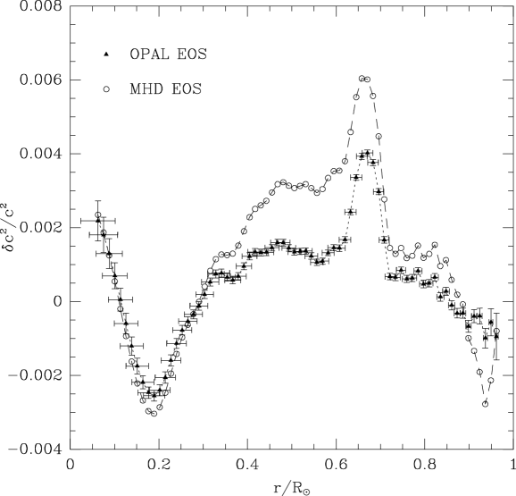
Figure 1: Difference between squared sound speed from inversion of oscillation data and that of a standard model based on the MHD (circles) and OPAL (triangles) equation of state (Figure provided by S. Basu).

In the solar convection zone, helioseismology presents an opportunity to isolate the question of the equation of state from opacity and nuclear reaction rates, since the stratification is essentially adiabatic and thus determined by thermodynamics (see, e.g., Christensen-Dalsgaard & Däppen (1992)). Accurate analysis of the observations requires use of the full, nonasymptotic behavior of the oscillations. Figure 1 shows a typical result of a numerical inversion (Basu & Christensen-Dalsgaard (1997)). It shows the relative difference (in the sense Sun – model) between the squared sound speed obtained from inversion of oscillation data and that of a two standard models. A perfect model would lie on the zero line. The two models are in all respects identical except that they use a different equation of state (MHD and OPAL, respectively, cf. Section 1). Simplifying for the present purpose, we can look at results such as shown in Figure 1 as the data of helioseismology, disregarding how they were obtained from solar oscillation frequencies.

The most important result of the earlier helioseismic equation-of-state analyses (Christensen-Dalsgaard et al. (1996)) was that it is essential to include the leading Coulomb correction (the Debye-Hückel term) to ideal-gas thermodynamics. Under solar conditions, the size of the relative Coulomb pressure correction is largest in the outer part of the convection zone (about –8 percent) and it has another local maximum in the core (about –1 percent). Figure 1, however, hides the fact that the Coulomb correction is the most important one, since both MHD and OPAL already contain it. Note that in Figure 1 the most significant information about the equation of state regards the convection zone ($r>0.71R_{\odot}$), since beneath it, one cannot disentangle the influence from the equation of state from other effects. Figure 1 contains the evidence that in the region $0.90R_{\odot}<r<0.97R_{\odot}$, OPAL is a better fit to reality than MHD.

Two very recent inversions have had further implications for the equation of state. First, the strong constraints from helioseismology now force us to include relativistic effects of electrons (Elliott & Kosovichev (1998)). Neither MHD nor OPAL have so far included relativistic effects, unlike the earlier and simpler EFF (Section 1) and its more recent sibling SIREFF (Guzik & Swenson (1997)). Second, there are indications that for $r>0.97R_{\odot}$, MHD is favored over OPAL. This is the result of an apparent helioseismic confirmation of the thermodynamic effect of the excited states in hydrogen, treated according to MHD [Eq. (4),(6)]. The effect itself was demonstrated in a theoretical study by Nayfonov & Däppen (1998), which revealed interesting features beyond the Coulomb correction approximation. They are related to excited states and their treatment in the equation of state. The MHD equation of state with its specific, density-dependent occupation probabilities (Section 2.3) is causing a characteristic “wiggle” in the thermodynamic quantities, most prominently in $\chi_{\rho}=(\partial\ln p/\partial\ln\rho)_{T}$, but equally present in the other thermodynamic quantities.

For convenience, in Figure The MHD equation of state with post-Holtsmark microfield distributions, we recall the result for the helioseismically relevant $\gamma_{1}$ of a hydrogen-only plasma. Temperatures and densities are taken from a solar model. The appropriate density is implied but not shown (for more details and different thermodynamic variables and chemical compositions, see Nayfonov & Däppen 1998 and Sections 6.2, 6.3). Five cases were considered: (i) ${\rm MHD}$ [standard MHD occupation probabilities: Eq. (4),(6)], (ii) ${\rm MHD_{GS}}$ [standard MHD internal partition function of hydrogen but truncated to the ground state (GS) term], (iii) ${\rm OPAL}$: OPAL tables [version of November 1996 of Rogers et al. (1996) (1996)], (iv) ${\rm MHD_{PL}}$ [MHD internal partition function of hydrogen, but replaced by the Planck-Larkin partition function $Z_{PL}=\sum_{1}^{\infty}g_{n}[\exp(-E_{n}/k_{\rm B}T)+E_{n}/k_{\rm B}T-1]$ (Rogers (1986))], (v) ${\rm MHD_{PL,GS}}$ [${\rm MHD_{PL}}$ truncated to the ground state term]. The effect of the inclusion of the excited states in the internal partition function is manifest in the differences between MHD and ${\rm MHD_{GS}}$, and between ${\rm MHD_{PL}}$ and ${\rm MHD_{PL,GS}}$, respectively. The effect of different occupation probabilities of ground and excited states shows up in the difference between MHD and ${\rm MHD_{PL}}$, and between ${\rm MHD_{GS}}$ and ${\rm MHD_{PL,GS}}$. It was found that the presence of excited states is crucial. Also, the wiggle was demonstrated to be a genuine neutral-hydrogen effect despite the fact that most hydrogen is already ionized. This qualitative picture does not change when helium is added Nayfonov & Däppen (1998).

It seems that this effect of excited states can be observed in the Sun. Figure 2 shows the result of the inversion by Basu et al. (1999), based on the solar oscillation frequencies obtained from the SOI/MDI instrument on board the SOHO spacecraft during its first 144 days in operation (Rhodes et al. 1997). Previous sound-speed and $\gamma_{1}$ inversions (e.g., Elliott & Kosovichev (1998)) were still indirect, that is, they were giving the difference between solar models and the Sun without separating the change in structure due to the equation-of-state contribution. The inversion by Basu et al. (1999) was done for the so-called “intrinsic” $\gamma_{1}$ difference between solar models and the Sun. For convenience, we repeat the principal result in Figure 2, which shows the difference between the Sun and various calibrated solar models. The models alternate between two equations of state (MHD, OPAL), three different values for the solar radius, and two formalisms for convection [MLT: standard mixing length theory, CM: Canuto & Mazitelli (1991) formalism]. The models are specified in Table 1, where in addition the calibrated values of the surface helium abundance $Y_{s}$ and the depth of the convection zone $r_{\rm cz}$ are listed. All models assume gravitational settling of helium and heavy elements, an effect that is now part of the so-called standard solar model (Christensen-Dalsgaard et al. (1996)).

In contrast to earlier results for the intrinsic $\gamma_{1}$ difference (Basu & Christensen-Dalsgaard (1997)), which had uniform resolution throughout the Sun, the new study focuses on the 20% uppermost layers. It appears that in the top layers, the MHD models give a more accurate description of the Sun than the OPAL models. Since the difference in $\gamma_{1}$ between MHD and OPAL is the wiggle of Figure The MHD equation of state with post-Holtsmark microfield distributions, the observed preference of the MHD model in the upper region could indicate a validation of an MHD-like treatment of the exited states. Fig. 2 confirms the aforementioned earlier findings that below the wiggle region, OPAL fares better than MHD. In that region, the Planck-Larkin partition function of OPAL appears to be the better choice.

The results in favor of MHD in the upper part of the Sun ($r>0.97R_{\odot}$) could be due to the different implementations of many-body interactions in the two formalisms. Since density decreases in the upper part, OPAL by its nature of a systematic expansion, inevitably becomes itself more accurate; but MHD might, by its heuristic approach, have incorporated even finer, higher-order effects.

Let us add a word of caution, though. It could appear tempting to produce a “combined” solar equation of state, with MHD for the top part and OPAL for the lower part. However, such a hybrid solution is fraught with danger. For instance, it is known that patching together equations of state can introduce spurious effects (Däppen et al. (1993)). It seems that the right way is to improve MHD and OPAL in parallel and independently, guided by the progress of helioseismology. The aim of the present study is to improve MHD.

4 Microfield Distributions

One of the mechanisms that affects the bound states of a radiator (atom or complex ion immersed in a plasma) is the electric field arising from the charged particles in its environment.

To be able to calculate the internal partition function it, therefore, is necessary to estimate $E_{nlm}$ and to calculate a microfield distribution. The actual electric field at a radiator in plasma is fluctuating in time. From the time-scale point of view, it is convenient to split the electric field into two components: a high-frequency part (with respect to the time scale of particle collisions) and a low-frequency component which varies on a time scale much longer than the orbital period of the bound state considered. Because of their high velocities, free electrons are considered as perturbers in the high-frequency part of the microfield distribution only. The distribution of the low-frequency component is calculated by considering a gas of ion perturbers. As was shown in (Hummer & Mihalas 1988), the low-frequency component dominates microfield effects at least for the conditions of stellar envelopes. In the following we discuss only this component.

4.1 Holtsmark Microfield Distribution

Unsöld (1948) suggested a model for a microfield distribution that allowed for a simple analytical formulation. It contained the nearest neighbor (NN) approximation and, therefore, was better suited to study the limit of strong fields. The long range of Coulomb interactions in plasmas, however, renders the nearest neighbor approximation inadequate. The next logical step in the development of the microfield distributions should involve the interaction of the radiator with all ions in plasma. For a case of pure hydrogen plasma this problem was worked out by Holtsmark (1919). Two serious shortcomings of the Holtsmark distribution are:

$\bullet$ its limitation to neutral radiators and

$\bullet$ the absence of correlations between the charged plasma perturbers.

The original MHD formalism (Hummer & Mihalas 1988) modified the Holtsmark distribution by making plausible but non-rigorous correction for the effects of ions other than protons. It considers hydrogenic radiators in a plasma for which the microfield perturbations by a variety of ionic species of charge $Z_{p}$, $p=1,2,$ are dominant. The resultant occupation probability of an electron in level $i$ = ($n,l,m$) of a hydrogenic potential of charge $Z_{a}$ is given by (see Eq. 4.68a of Hummer & Mihalas 1988)

$$w_{i}^{c}=Q\left[{{K_{i}\chi_{i}^{2}}\over{4Z_{a}a_{0}^{3}}}{\left({4\pi n_{e}\over 3}\right)}^{-2/3}{\left(n_{ion}\over n_{e}\right)}^{1/3}\right]\ ,$$ (8)

where

$$Q(x)=\int_{0}^{x}P_{H}(\beta)d\beta\ ,$$ (9)

$K_{i}$ is the quantal Stark-ionization correction factor, $\chi_{i}$ is the ionization potential of the level $i$, $a_{0}$ is the Bohr radius, $n_{e}$ is the electron density, $n_{ion}$ is the density of all ions, and $P_{H}(\beta)$ is the Holtsmark distribution function

$$P_{H}(\beta)=\left(2\beta\over\pi\right){\int_{0}^{\infty}}dy\exp(-y^{3/2})y\sin\beta y.$$ (10)

4.2 MHD Microfield Distribution

In the form of Eq. (8) the calculations of plasmas with dozens of ions and hundreds of bound states are too cumbersome, especially if one wants to code all the derivatives in the analytical form. Instead, MHD relied on numerical experiments in search for analytical fits that would mimic the Holtsmark distribution function. It turned out that a good starting point was the Unsöld (1948) occupation probability $w_{i}^{c}$, given by

$$w_{i}^{c}=\exp\left(-{32\pi\over{3V}}{Z_{a}^{3/2}a_{0}^{3}\over{K_{i}^{3/2}\chi_{i}^{3}}}\sum_{p}N_{p}Z_{p}^{3/2}\right).$$ (11)

It might be worth noting here that because $\chi_{i}\propto 1/n^{2}$, even putting the arbitrary factor of 2 into exponent of Eq. (11) changes the cutoff quantum number by only a factor of $2^{1/6}=1.12$, which is typically quite negligible.

This simple expression is indeed a good fit to the Holtsmark distribution, if an additional more-or-less ad hoc factor 2 is put in the argument of Eq.(8). Tests showed (Hummer & Mihalas 1988) that for strongly bound states with $w_{i}^{c}\geq 0.1$ this trick actually leads to a good fit. However, for $w_{i}^{c}\leq 0.1$ this fit decreases much more sharply than does Eq.(8); for many applications this is not a matter of serious concern inasmuch as the basic physical effect - that such levels are for all practical purposes destroyed - is achieved.

The adopted form of $w_{i}^{c}$ in MHD equation of state reflects the interactions of the radiator with all ions in the plasma, but the approximation does not take into account the correlations of the charged perturbers. This effect is already a problem because of the choice of the Holtsmark distribution function, not only one of the replacement of the Holtsmark distribution by a modified Unsöld expression (Iglesias & Rogers 1995).

4.3 Microfield Distributions with Correlation Effects

4.3.1 APEX Microfield Distribution

One of the alternative methods to calculate the microfield distribution for plasmas of general nature, which include particle correlations, is the APEX (“adjustable-parameter exponential”) approximation ( see Iglesias et al. (1985) and references therein) based on a so-called “independent quasiparticle model”.

Originally developed as a phenomenological method, APEX was shown to be in agreement with a rigorous theoretical procedure (Dufty et al. (1985)) related to a Baranger-Mozer series type of analysis. APEX has been shown to agree quite well with computer Monte-Carlo simulations for both high- and low-frequency component distributions. Especially well-suited for high-Z plasmas (Iglesias et al. (1983)), it treats the low-frequency component by considering a gas of ions interacting through electron screened potentials, which is a way to include static contributions from both ions and electrons into account. The success of APEX can be attributed to a fact that for small fields the contributions from many ions are important and these are well characterized by the second moment of the microfield distribution that is exactly included in APEX.

The correlation effects are incorporated through the radial distribution functions of the ionic perturbers calculated in the hyper-netted-chain approximation generalized to multi-component plasmas (Rogers (1980)).

4.3.2 Q-fit Microfield Distribution

An alternative improvement over the Holtsmark distribution function, which accounted for particle correlations yet remained sufficiently simple so that it could be expressed by analytical fits suited to an equation-of-state program, was introduced by one of the authors (D. Hummer) in 1990. The numerical fits were based on work by Hooper (1966, 1968). Although until the present work these fits have never been included in equation of state calculations, they were successfully used in an non-LTE investigation of the stellar flux near the series limits in hot stars (Hubeny, Hummer & Lanz (1994)).

The Hooper (1966, 1968) microfield distribution was derived under the following assumptions:

$\bullet$ the perturbing ions and electrons are in equilibrium with the same kinetic temperature,

$\bullet$ while multiply charged radiators were allowed, all of the perturbing ions were singly charged.

While these assumptions are obviously too stringent for studies of general plasmas and even laser-generated plasmas (see Tighe & Hooper (1977)), they should be quite reasonable for the plasma of the interior of more or less normal stars having typical astrophysical compositions. In this case, one can show that the two assumptions of the Hooper microfield are indeed satisfied. First, the interior of normal stars is in thermodynamic equilibrium. Electrons and ions have therefore the same temperature. Note that stellar atmospheres are of course not in thermal equilibrium, but any stellar equation of state of the type discussed in this article is inadequate for them, and special nonlocal formalisms are needed. Second, for not-too-evolved stars, the typical chemical composition of the universe prevails, which has about 90% hydrogen by number. For such plasmas, the vast majority of perturbing ions are protons, i.e., singly charged.

When plasma correlation effects are important, the microfield distribution function depends on two additional parameter, the radiator charge $Z_{r}$ and the correlation parameter

$$a={\left({4\pi\over 3}n_{e}r_{D}^{3}\right)}^{-1/3}=\ {0.09n_{e}^{1/6}\over{T^{1/2}}}\ ,$$ (12)

where $n_{e}$ is in ${\rm cm}^{-3}$ and $T$ is in $K$.

The physical meaning of the parameter $a$ is clear from Eq. (12), namely $a=\eta^{-1/3}$, where $\eta$ is the number of ions in a Debye sphere of radius $r_{D}$

$$r_{D}=\sqrt{k_{\rm B}T\over{4\pi e^{2}n_{e}}}.$$ (13)

In the low-frequency approximation only electrons contribute to shielding [Eq. (13)] and the overall charge neutrality of plasma was used to obtain the last form of Eq. (12).

Another way to look at $a$ is to realize that it can be expressed in terms of the electron coupling parameter $\Gamma_{\rm e}$:

$$a^{2}=3\left({e^{2}\over{k_{\rm B}Ta_{e}}}\right)=3\Gamma_{\rm e}\ ,$$ (14)

where $a_{e}$ is the electron sphere radius defined by ${4\pi\over 3}n_{e}a_{e}^{3}=1$.

The appropriate microfield distribution function $W(\beta;Z_{r},a)$ has been derived by Hooper (1966, 1968). Using a substantially modified version of Hooper’s code, Thomas Schöning of the University of Munich Observatory and Hummer computed two-dimensional fits in $\beta$ and $a$ to $W(\beta;Z_{r},a)$ for $Z_{r}=0,\ldots,5$ and $a\leq 0.8$. From these fits Hummer evaluated the function defined by Eq. (9)

$$Q(\beta;Z_{r},a)\equiv\int_{0}^{\beta}W(\beta^{\prime};Z_{r},a)d\beta^{\prime}$$ (15)

for the given ranges of the parameters $Z_{r}$ and $a$. It was possible to get a reasonably good analytical fit to obtained data by using just two parameters: radiative charge $Z_{r}$ and a correlation parameter $a$.

The adopted form of the fit $Q(\beta,Z_{r},a)$ is

$$Q(\beta,Z_{r},a)={f(\beta,Z_{r},a)\over{1+f(\beta,Z_{r},a)}},$$ (16)

where

$$f(\beta,Z_{r},a)={C_{1}(Z_{r},a)\beta^{3}\over{1+C_{2}(Z_{r},a)\beta^{3/2}}}.$$ (17)

The coefficients $C_{1}$ and $C_{2}$ depend on $a$ and $Z_{r}$ through the forms:

$$C_{1}(Z_{r},a)=P_{1}\left[X+P_{5}Z_{r}a^{3}\right]\ ,$$ (18)

and

$$C_{2}=P_{2}X,$$ (19)

where

$$X={(1.0+P_{3}a)}^{P_{4}}\ ,$$ (20)

and the optimum values of the parameters seem to be:

$$P_{1} = 0.1402$$

$$P_{2} = 0.1285$$

$$P_{3} = 1.0$$ (21)

$$P_{4} = 3.15$$

$$P_{5} = 4.0\ .$$

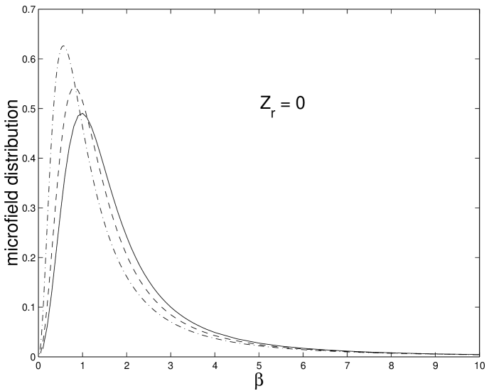
Figure 3: Microfield distribution from Q-MHD model in a case of neutral perturber in hydrogen plasma for different values of coupling parameter: $\Gamma$ = 0.10 (solid line), $\Gamma$ = 0.25 (dashed line), $\Gamma$ = 1.0 (dotted-dashed line).

The chosen forms of the fits are constrained to lie between zero and 1 for all values of $a$ and $Z_{r}$ and to give the correct functional form for both small and large limiting values of $\beta$. The presented fits have been obtained for data from $a=0$ (no correlation, which corresponds to the Holtsmark limit) to $a=0.8$. For $a$=$Z_{r}$=0, the fit is accurate to within $\pm 2\%$. Except for very small values of $\beta$, the fit is accurate to within 10$\%$, except for large $a$ and $Z_{r}$, where it reaches 26$\%$ in the worst case ( for very small $\beta$). However, as $Q(\beta)$ is very small there ( on the order of $10^{-4}$ ), it shouldn’t matter. Figures 3 and 5 demonstrate the magnitude of the correlation effects for a neutral as well as for a singly charged radiator.

In the following we are going to ignore the temperature and density dependence of the coefficients $C_{1}$,$C_{2}$ in the derivatives of the $Q(\beta)$. For solar conditions, the maximum relative error of this approximation is about $10^{-3}$-$10^{-4}$ and, therefore, the approximation is quite sufficient for our fits, which in any case have a few percent errors themselves. Henceforth,

$${df\over{d\beta}}={3C_{1}{\beta}^{2}(1+{1\over 2}C_{2}{\beta}^{3/2})\over{{(1+C_{2}{\beta}^{3/2})}^{2}}}\ ,$$ (22)

$${d^{2}f\over{d^{2}\beta}}={3\over 4}C_{1}\beta{(8+3C_{2}{\beta}^{3/2}+C_{2}^{2}{\beta}^{3})\over{{(1+C_{2}{\beta}^{3/2})}^{3}}}\ ,$$ (23)

$$Q^{{}^{\prime}}(\beta)={1\over{{(1+f)}^{2}}}{\left({df\over{d\beta}}\right)}\ ,$$ (24)

$$Q^{{}^{\prime\prime}}(\beta)={1\over{{(1+f)}^{2}}}{\left[{{d^{2}f\over{d^{2}\beta}}-{2\over{(1+f)}}{\left({df\over{d\beta}}\right)}^{2}}\right]}\ .$$ (25)

5 Q-MHD Equation of State

5.1 Q-fit Occupation Probability

The post-Holtsmark microfield distribution given by the Q-fit can be used to upgrade the original MHD to the Q-MHD equation of state. Recall (Section 2.3) that the MHD-style occupation probability is given by a product of neutral and charged parts

$$w_{ijk}=w_{ijk}^{c}w_{ijk}^{n}\ .$$ (26)

The neutral part $w_{ijk}^{n}$, corresponding to pressure ionization mechanism, has the same form as in the original MHD representation (see Hummer & Mihalas 1988). The charged part $w_{ijk}^{c}$, determined by the microfield distribution, is given by

$$w_{ijk}^{c}=Q(\beta_{ijk})\ ,$$ (27)

$$\beta_{ijk}={\left(3\over{4\pi}\right)}^{2/3}{K_{ijk}\chi_{ijk}^{2}\over{4(Z_{jk}+1)e^{4}}}{\left({n_{ion}\over n_{e}}\right)}^{1/3}{1\over{n_{e}^{2/3}}}\ ,$$ (28)

where $\chi_{ijk}$ is the ionization potential of level $i$ of ion $j$ of chemical species $k$, $Z_{jk}$ is the net charge on ion $j$ of species $k$ ( zero for neutral particle), $n_{ion}$ is the total density of ionic perturbers in a system and $n_{e}$ is again the electron density. $K_{n}$ is the quantal Stark-ionization correction factor of MHD theory (see Hummer & Mihalas 1988)

$$K_{n} = 1\ ,\ \ n\leq 3,$$

$$K_{n} = {16\over 3}{n\over{(n+1)}^{2}}\ ,\ \ n>3\ .$$ (29)

In the following we adopt an important approximation ${\left({n_{ion}/{n_{e}}}\right)}^{1/3}\approx 1$. As been already discussed in Hummer & Mihalas (1988) the error of this assumption for stellar plasmas of normal chemical compositions never exceeds a few percent due to scarcity of high-Z species. This minor approximation simplifies the analytical derivatives (Appendix) significantly.

Therefore, Equation (28) can be rewritten as

$$\beta_{ijk}=\beta_{ijk}(n_{e})={\left(3\over{4\pi}\right)}^{2/3}{K_{ijk}\chi_{ijk}^{2}\over{4(Z_{jk}+1)e^{4}}}{n_{e}^{-2/3}}\ .$$ (30)

5.2 Q-MHD Free Energy

Once the new Q-fit occupation probabilities are known, they merely have to be put in place of the original MHD occupation probabilities. To allow detailed comparisons with the MHD expressions (Mihalas et al. (1988); Däppen et al. (1988)), we list the Q-fit analogs in the Appendix. Calculation of the ionization equilibria and thermodynamic quantities is done as in MHD, and the result is the Q-MHD equation of state.

6 Results and Discussion

6.1 Comparisons of Q-fit and APEX Microfield Distributions

In this section the microfield distributions in hydrogen plasmas are presented for different values of the plasma coupling parameter $\Gamma$ (which is the ionic analog to $\Gamma_{\rm e}$ defined by Eq. (14). More precisely,

$$\Gamma=\left({e^{2}\over{k_{\rm B}Ta_{\rm av}}}\right)\ ,$$ (31)

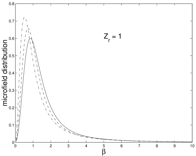
Figure 5: Same as Fig.1 in a case of $Z_{r}=1$ perturber.

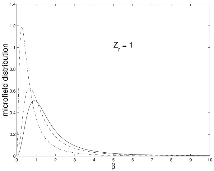
Figure 6: Same as Fig.2 in a case of $Z_{r}=1$ perturber.

where $a_{\rm av}$ is the average ion sphere radius defined by $({4\pi/3})\sum_{\rm ion}n_{i}a_{\rm av}^{3}=1$. In both Q-MHD and APEX formalisms only singly-charged perturbers considered. To demonstrate the effect of a radiator charge, the case of a neutral ($Z_{r}=0$) radiator (see Figs. 3 and 4) is presented alongside with the singly-charged ($Z_{r}=1$) case (Figs. 5-6) calculated for a several values of coupling parameter $\Gamma$.

The resultant function Q [see Eq. (9)] for these cases demonstrates a clear dependence on a radiator charge as well as on a value of $\Gamma$.

6.2 Comparison of the Equation of State for a Hydrogen-only Plasma

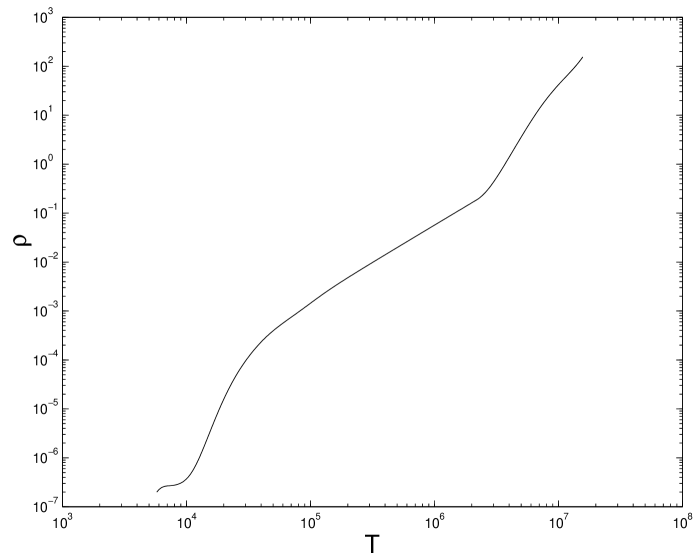
Figure 11: “H-only solar track”: for given temperature, density of a hydrogen-only plasma is chosen such that pressure corresponds to solar pressure.

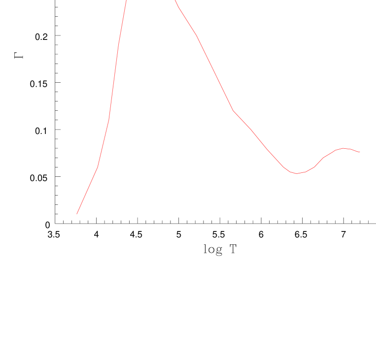
Figure 12: Estimated coupling parameter $\Gamma$ along the H-only solar track

This section deals with equation-of-state calculations for hydrogen-only plasmas. Four different equations of state have been calculated for a set of fictitious solar temperatures and densities, given in Fig. 11. The densities were chosen by Nayfonov & Däppen (1998) to simulate solar pressure at the given temperature for a hydrogen-only plasma. In the following we will denote by “H-only solar track” the set of temperatures and densities of Figure 11. Figure 12 demonstrates a coupling parameter $\Gamma$ as estimated for the conditions of the H-only solar track.

The four equations of state (EOS) are: (i) regular MHD EOS (solid lines in all of the following graphs); (ii) MHD EOS with a true Holtsmark microfield distribution function (dotted-dashed lines); (iii) Q-MHD EOS, as described in Section 5 of this paper (dashed lines) and, finally, (iv) OPAL EOS (dotted lines). The results expand the previous study (Nayfonov & Däppen 1998) on the effects of internal partition functions, and in as much as the studies overlap, they agree with each other. Among the quantities considered, that is, $\chi_{\rho}={(\partial\ln p/\partial\ln\rho)}_{T}$, $\chi_{T}={(\partial\ln p/\partial\ln T)}_{\rho}$, and $\gamma_{1}={(\partial\ln p/\partial\ln\rho)}_{s}$, only $\chi_{\rho}$ reveals differences already in the absolute plot. However, the differences are present, and of the same order of magnitude, also in the other two quantities, in the same way as found by Nayfonov & Däppen (1998). Figures 13 and 14 show absolute values of $\chi_{\rho}$ and relative difference (with respect to OPAL), respectively. All three MHD-type EOS (i.e., MHD, MHD with true Holtsmark, and Q-MHD) demonstrate the characteristic wiggle discovered in the previous study (see also Fig. The MHD equation of state with post-Holtsmark microfield distributions). The wiggle is located in the temperature zone $4.5\leq\log T\leq 5.3$. Given the hydrogen-only plasma, it is obviously a pure hydrogen phenomenon. However, as the location of the 10% to 90% ionization zone demonstrates (Fig. 14), the wiggle is caused by the last remaining neutral hydrogen atoms, fighting against pressure ionization in a region of near full ionization.

The figures also reveal a close agreement between regular MHD and MHD with a true Holtsmark distribution function, which gives a post factum justification of the choice made by the authors of MHD in 1988. It is also clear that Q-MHD seems to be in a better overall agreement with OPAL than other two equations of state.

6.3 Comparison of the Equation of State for a Hydrogen-Helium Mixture

To study a more realistic picture of solar plasmas, calculations similar to ones described in the previous section were carried out for a hydrogen-helium mixture along a real solar profile of density and temperature (model S of Christensen-Dalsgaard et al. (1996)). Hydrogen constitutes 74% of this mixture by mass, making it very similar to a solar composition of the standard solar model. While those calculations exclude heavier elements from the analysis, the obtained results actually give a strong indication that a treatment of heavier elements is necessary to improve our current equation of state models (Däppen et al. (1993)). The plots of absolute values of $\chi_{\rho}$ and of relative differences (with respect to OPAL) between the same four equations of state are given by Figures 15 and 16.

Figure 17 reveals that the signature of the hydrogenic internal partition function is present in other thermodynamic quantities, such as $\gamma_{1}$, as well. Again, one can argue that Q-MHD agrees with OPAL better than the other models and that the differences between the usual MHD and MHD with a true Holtsmark distribution remain small. Fig. 17 shows that Q-MHD leaves MHD and approaches OPAL especially in the temperature range $5.1\leq\log T\leq 5.4$. From the comparison with the helioseismic experiment (Fig. 2), one realizes that for at least the upper part of this temperature range, OPAL is a better equation of state than MHD. Therefore, Q-MHD corrects MHD in the right direction.

7 Conclusion

Upgrading the MHD equation of state to include realistic microfield distributions beyond the Holtsmark approximation has confirmed the significant changes in the occupation numbers for atomic and ionic states, as was expected by Iglesias & Rogers (1995). These changes in the occupation numbers and the associated shifts in the ionization balances are widely assumed responsible, among other, for the discrepancies between OP and OPAL opacities under the temperatures and densities of the solar center (see Gong et al. (1998)). For conditions of envelopes of more massive stars, however, the two opacity calculations agree very well. Our study is a systematic comparison of the impact on occupation probabilities of the original MHD microfield, the proper Holtsmark microfield, and the APEX distribution.

As far as thermodynamic properties are concerned, Iglesias & Rogers (1995) and also Rogers & Iglesias (1998) believed that effects of different microfield distributions would be rather negligible. But encouraged by recent progress on the influence of excited states in hydrogen on thermodynamic quantities (Section 3), we have found a clear signature of the microfield distribution, easily within reach of helioseismological accuracy (compare Figures 2 and 17). This confirms once more that solar observations constrain formalisms used to describe the physics of atoms and compound ions immersed in a plasma.

Since these thermodynamic effects are nonetheless quite small and are, even for helioseismological accuracy, only relevant at some selected locations of the Sun, our results also show that for most applications of stellar structure, the approximations chosen in the original MHD equation of state are reasonable. In the particular cases where they are not reasonable, such as in helioseismological studies of the zones of partial ionization in the Sun, the more accurate Q-MHD equation of state, which is based on a realistic microfield distribution, is more accurate.

8 Acknowledgments

We thank Jørgen Christensen–Dalsgaard, Carlos Iglesias and Forrest Rogers for stimulating discussions and critical comments. We are grateful to Sarbani Basu for providing Figures 1 and 2. A.N. and W.D. are supported by the grant AST-9618549 of the National Science Foundation. W.D. acknowledges additional support from the SOHO Guest Investigator Grant NAG5-7352 of NASA, the Danish National Research Foundation through its establishment of the Theoretical Astrophysics Center, and from PPARC. D.M. was supported by the Mc Vittie Professorship Fund at the University of Illinois during the early phases of this work. SOHO is a project of international cooperation between ESA and NASA.

Appendix A Appendix: Analytical Expressions for the Free Energy and Its Derivatives with Q-fit Occupation Probabilities

We follow the MHD notation (Mihalas et al. (1988); Däppen et al. (1988)) very closely. The term affected by the new microfield is the free energy of bound systems of species $s$

$$F_{2}=\sum_{s\neq e}N_{s}\left(E_{1s}-k_{\rm B}T\log Z_{s}\right)\ ,$$ (A1)

with the internal partition function evaluated for energies relative to the ground state, that is,

$$Z_{s}=\sum_{i}w_{is}g_{is}\exp\left({-\Delta E_{is}\over{k_{\rm B}T}}\right)\ .$$ (A2)

Here, $\Delta E_{is}=E_{is}-E_{1s}$. In what follows, $\lambda,\mu,\nu$ label neutral, $q$ charged particles. We shall also treat ($N_{p}/N_{e})$ as a constant (see the discussion leading to Eq. (30). Then, (1) $F_{2}$ is linear in $N_{j}$, and (2), $Z_{s}$ does not depend on individual ions $N_{j}$. Then

$${\partial F_{2}\over{\partial N_{\nu}}}=E_{1\nu}-k_{\rm B}T\ln Z_{\nu}-k_{\rm B}T\sum_{s\neq e}{N_{s}\over Z_{s}}{\partial Z_{s}\over{\partial N_{\nu}}}$$ (A3)

$${\partial F_{2}\over{\partial N_{q}}}=E_{1q}-k_{\rm B}T\ln Z_{q}$$ (A4)

$${\partial F_{2}\over{\partial N_{e}}}=-k_{\rm B}T\sum_{s\neq e}{N_{s}\over Z_{s}}{\partial Z_{s}\over{\partial N_{e}}}$$ (A5)

$${\partial^{2}F_{2}\over{\partial N_{e}^{2}}}=-k_{\rm B}T\sum_{s\neq e}{N_{s}\over Z_{s}}{\left[{{\partial^{2}Z_{s}\over{\partial N_{e}^{2}}}-{1\over{Z_{s}}}{\left({\partial Z_{s}\over{\partial N_{e}}}\right)}^{2}}\right]}$$ (A6)

$${\partial^{2}F_{2}\over{\partial N_{e}\partial N_{q}}}=-k_{\rm B}T{1\over{Z_{q}}}{\partial Z_{q}\over{\partial N_{e}}}$$ (A7)

$${\partial^{2}F_{2}\over{\partial N_{\lambda}\partial N_{e}}}=-k_{\rm B}T\left[{1\over{Z_{\lambda}}}{\partial Z_{\lambda}\over{\partial N_{e}}}+\sum_{s\neq e}{N_{s}\over Z_{s}}\left({\partial^{2}Z_{s}\over{\partial N_{e}\partial N_{\lambda}}}-{1\over{Z_{s}}}{{\partial Z_{s}\over{\partial N_{e}}}}{{\partial Z_{s}\over{\partial N_{\lambda}}}}\right)\right]$$ (A8)

$${\partial^{2}F_{2}\over{\partial N_{\lambda}\partial N_{\mu}}}=-k_{\rm B}T\left[{1\over{Z_{\lambda}}}{\partial Z_{\lambda}\over{\partial N_{\mu}}}+{1\over{Z_{\mu}}}{\partial Z_{\mu}\over{\partial N_{\lambda}}}+\sum_{s\neq e}{N_{s}\over Z_{s}}\left({\partial^{2}Z_{s}\over{\partial N_{\mu}\partial N_{\lambda}}}-{1\over{Z_{s}}}{\partial Z_{s}\over{\partial N_{\mu}}}{\partial Z_{s}\over{\partial N_{\lambda}}}\right)\right]$$ (A9)

$${\partial^{2}F_{2}\over{\partial T\partial N_{e}}}=-k_{\rm B}T\sum_{s\neq e}{N_{s}\over Z_{s}}{\left[{{\partial^{2}Z_{s}\over{\partial N_{e}\partial T}}+{\left({{1\over T}-{1\over Z_{s}}{\partial Z_{s}\over{\partial T}}}\right)}{\partial Z_{s}\over{\partial N_{e}}}}\right]}$$ (A10)

$${\partial^{2}F_{2}\over{\partial T\partial N_{\lambda}}}=-k_{\rm B}T{\left\{{{1\over T}\ln Z_{\lambda}+{1\over{Z_{\lambda}}}{\partial Z_{\lambda}\over{\partial T}}+\sum_{s\neq e}{N_{s}\over Z_{s}}{\left[{{\partial^{2}Z_{s}\over{\partial T\partial N_{\lambda}}}+{\left({{1\over T}-{1\over Z_{s}}{\partial Z_{s}\over{\partial T}}}\right)}{\partial Z_{s}\over{\partial N_{\lambda}}}}\right]}}\right\}}$$ (A11)

$${\partial^{2}F_{2}\over{\partial T\partial N_{q}}}=-k_{\rm B}T\left({1\over T}\ln Z_{q}+{1\over{Z_{q}}}{\partial Z_{q}\over{\partial T}}\right)$$ (A12)

$${\partial^{2}F_{2}\over{\partial V\partial N_{\lambda}}}=-k_{\rm B}T\left[{1\over{Z_{\lambda}}}{\partial Z_{\lambda}\over{\partial V}}+\sum_{s\neq e}{N_{s}\over Z_{s}}\left({\partial^{2}Z_{s}\over{\partial V\partial N_{\lambda}}}-{1\over{Z_{s}}}{\partial Z_{s}\over{\partial V}}{\partial Z_{s}\over{\partial N_{\lambda}}}\right)\right]$$ (A13)

$${\partial^{2}F_{2}\over{\partial V\partial N_{e}}}=-k_{\rm B}T\sum_{s\neq e}{N_{s}\over Z_{s}}\left({\partial^{2}Z_{s}\over{\partial V\partial N_{e}}}-{1\over{Z_{s}}}{\partial Z_{s}\over{\partial V}}{\partial Z_{s}\over{\partial N_{e}}}\right)$$ (A14)

$${\partial^{2}F_{2}\over{\partial V\partial N_{q}}}=-{k_{\rm B}T\over Z_{q}}{\partial Z_{q}\over{\partial V}}$$ (A15)

$${\partial Z_{s}\over{\partial N_{e}}}=-{2\over{3N_{e}}}\sum_{i}{\beta_{is}Q_{is}^{{}^{\prime}}\over{Q_{is}}}w_{is}g_{is}e^{{-\Delta E_{is}/{k_{\rm B}T}}}$$ (A16)

$${\partial^{2}Z_{s}\over{\partial N_{e}^{2}}}=-{\left(\frac{2}{3N_{e}}\right)}^{2}\sum_{i}{\beta_{is}^{2}\over{Q_{is}}}{\left({Q_{is}^{{}^{\prime\prime}}+{5\over 2}{Q_{is}^{{}^{\prime}}\over{\beta_{is}}}}\right)}w_{is}g_{is}e^{{-\Delta E_{is}/{k_{\rm B}T}}}$$ (A17)

$${\partial Z_{\nu}\over{\partial N_{\mu}}}=-{4\pi\over{3V}}\sum_{i}{(r_{i\nu}+r_{1\mu})}^{3}w_{i\nu}g_{i\nu}e^{{-\Delta E_{i\nu}/{k_{\rm B}T}}}$$ (A18)

$${\partial^{2}Z_{\nu}\over{\partial N_{\mu}\partial N_{\lambda}}}={\left({4\pi\over{3V}}\right)}^{2}\sum_{i}{(r_{i\nu}+r_{1\mu})}^{3}{(r_{i\nu}+r_{1\lambda})}^{3}w_{i\nu}g_{i\nu}e^{{-\Delta E_{i\nu}/{k_{\rm B}T}}}$$ (A19)

$${\partial^{2}Z_{\nu}\over{\partial N_{\mu}\partial N_{e}}}={8\pi\over{9N_{e}V}}\sum_{i}{(r_{i\nu}+r_{1\mu})}^{3}{\left({\beta_{i\nu}Q_{i\nu}^{{}^{\prime}}\over{Q_{i\nu}}}\right)}w_{s\nu}g_{i\nu}e^{{-\Delta E_{i\nu}/{k_{\rm B}T}}}$$ (A20)

$${\partial Z_{s}\over{\partial T}}={1\over{k_{\rm B}T^{2}}}\sum_{i}{\Delta E_{is}}w_{is}g_{is}e^{{-\Delta E_{is}/{k_{\rm B}T}}}$$ (A21)

$${\partial^{2}Z_{s}\over{\partial T^{2}}}={\left({1\over{k_{\rm B}T^{2}}}\right)}^{2}\sum_{i}{\Delta E_{is}}{\left({\Delta E_{is}-2k_{\rm B}T}\right)}w_{is}g_{is}e^{{-\Delta E_{is}/{k_{\rm B}T}}}$$ (A22)

$${\partial^{2}Z_{s}\over{\partial T\partial N_{e}}}=-{2\over{3k_{\rm B}T^{2}N_{e}}}\sum_{i}{\Delta E_{is}}{\left({\beta_{is}Q_{is}^{{}^{\prime}}\over{Q_{is}}}\right)}w_{is}g_{is}e^{{-\Delta E_{is}/{k_{\rm B}T}}}$$ (A23)

$${\partial^{2}Z_{s}\over{\partial T\partial N_{\mu}}}=-{4\pi\over{3k_{\rm B}T^{2}V}}\sum_{i}{\Delta E_{is}}{(r_{is}+r_{1\mu})}^{3}w_{is}g_{is}e^{{-\Delta E_{is}/{k_{\rm B}T}}}$$ (A24)

$${\partial Z_{s}\over{\partial V}}={1\over{V}}\sum_{i}\left[{2\beta_{is}Q_{is}^{{}^{\prime}}\over{3Q_{is}}}+\frac{4\pi}{3V}\sum_{\nu}N_{\nu}(r_{is}+r_{1\nu})^{3}\right]w_{is}g_{is}e^{-\Delta E_{is}/{k_{\rm B}T}}$$ (A25)

$${\partial^{2}Z_{s}\over{\partial T\partial V}}={1\over{k_{\rm B}T^{2}V}}\sum_{i}\Delta E_{is}{\left[{{2\beta_{is}Q_{is}^{{}^{\prime}}\over{3Q_{is}}}+\frac{4\pi}{3V}\sum_{\nu}N_{\nu}(r_{is}+r_{1\nu})^{3}}\right]}w_{is}g_{is}e^{{-\Delta E_{is}/{k_{\rm B}T}}}$$ (A26)

$${\partial^{2}Z_{s}\over{\partial V\partial N_{\mu}}}=\frac{4\pi}{3V^{2}}\sum_{i}{(r_{is}+r_{1\mu})}^{3}\hskip 199.16928pt$$

$$\;\;\;\;\;\;\;\;\;\;\;\;\;\;\;\;\;\;\;\;\;\;\;\;\;\;\;\;\;\;\;\;\;\;\;\;{\left\{{-{2\over 3}{\beta_{is}Q_{is}^{{}^{\prime}}\over{Q_{is}}}+{\left[{1-{4\pi\over{3V}}\sum_{\nu}N_{\nu}{(r_{is}+r_{1\nu})}^{3}}\right]}}\right\}}w_{is}g_{is}e^{{-\Delta E_{is}/{k_{\rm B}T}}}$$ (A27)

$${\partial^{2}Z_{s}\over{\partial V\partial N_{e}}}=-\frac{2}{3N_{e}V}\sum_{i}\left\{{\frac{4\pi}{3V}{\beta_{is}Q_{is}^{{}^{\prime}}\over{Q_{is}}}\left[\sum_{\nu}N_{\nu}(r_{is}+r_{1\nu})^{3}\right]}\right.\hskip 170.71652pt$$

$$\;\;\;\;\;\;\;\;\;\;\;\;\;\;\;\;\;\;\;\;\;\;\;\;\;\;\;\;\;\;\;\;\;\;\;\;\;\;\;\left.+\frac{2}{3}\sum_{i}{\beta_{is}\over{Q_{is}}}(Q_{is}^{{}^{\prime}}+\beta_{is}Q_{is}^{{}^{\prime\prime}})\right\}w_{is}g_{is}e^{{-\Delta E_{is}/{k_{\rm B}T}}}$$ (A28)

$${\partial^{2}Z_{s}\over{\partial V^{2}}}={1\over V^{2}}\sum_{i}\left\{\left[\frac{4\pi}{3V}\sum_{\nu}N_{\nu}(r_{is}+r_{1\nu})^{3}\right]\left[{4\over 3}{\beta_{is}Q_{is}^{{}^{\prime}}\over{Q_{is}}}+\left(\frac{4\pi}{3V}\sum_{\nu}N_{\nu}(r_{is}+r_{1\nu})^{3}-2\right)\right]\right.\hskip 28.45274pt$$

$$\;\;\;\;\;\;\;\;\;\;\;\;\;\;\;\;\;\;\;\;\;\;\;\;\;\;\;\;\;\;\;\;\;\;\;\;\;\;\;\;\;\;\;\;\;\;\;\;\;\;\;\;\;\;\;\;\;\;\left.+{4\over 9}{\beta_{is}\over{Q_{is}}}(\beta_{is}Q_{is}^{{}^{\prime\prime}}-{1\over 2}Q_{is}^{{}^{\prime}})\right\}w_{is}g_{is}e^{-\Delta E_{is}/{k_{\rm B}T}}$$ (A29)

Table 1: Properties of the solar models of Fig. 2. See text.

Model	EOS	Radius	Convective	$Y_{s}$	$r_{\rm cz}/R_{\odot}$
		Mm	Flux
M1	MHD	695.78	CM	0.2472	0.7145
M2	MHD	695.99	CM	0.2472	0.7146
M3	MHD	695.51	CM	0.2472	0.7145
M4	MHD	695.78	MLT	0.2472	0.7146
M5	OPAL	695.78	CM	0.2465	0.7134
M6	OPAL	695.99	CM	0.2465	0.7135
M7	OPAL	695.51	CM	0.2466	0.7133
M8	OPAL	695.78	MLT	0.2465	0.7135

Left Panel: absolute values of $\gamma_{1}$ for solar temperatures and densities of a hydrogen-only plasma. Linestyles: MHD – asterisks, ${\rm MHD_{GS}}$ – dashed lines, ${\rm MHD_{PL}}$ – dotted-dashed lines, ${\rm MHD_{PL,GS}}$ – dotted lines, and OPAL – solid lines. See text for the definitions of the different MHD versions. Right Panel: relative differences with respect to ${\rm MHD_{GS}}$, in the sense $(\gamma_{1}-\gamma_{1}[{\rm MHD_{GS}}])/\gamma_{1}[{\rm MHD_{GS}}])$, using the same line styles as in the left panel. The horizontal solid zero line, representing ${\rm MHD_{GS}}$, is also shown.

Figure 2: Relative difference between $\gamma_{1}$ obtained from an inversion of helioseismological data and $\gamma_{1}$ of the solar models listed in Table I, in the sense “Sun – model”. Only the intrinsic difference in $\gamma_{1}$ is shown, that is, the part of the difference due to the equation of state (Figure provided by S. Basu).

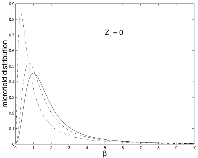
Figure 4: Microfield distribution from APEX model in a case of neutral perturber in hydrogen plasma for different values of coupling parameter: $\Gamma$ = 0.10 (solid line), $\Gamma$ = 0.25 (dashed line), $\Gamma$ = 1.0 (dotted-dashed line).

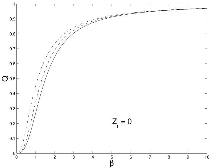
Figure 7: Function Q for a case presented in Fig.1

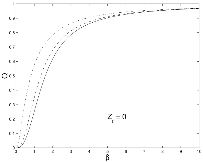
Figure 8: Function Q for a case presented in Fig.2

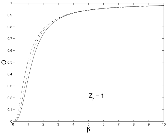
Figure 9: Function Q for a case presented in Fig.3

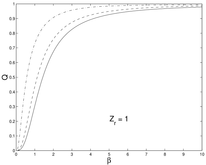
Figure 10: Function Q for a case presented in Fig.4

Figure 13: $\chi_{\rho}$ for a case of hydrogen-only plasma calculated for 4 different models: standard MHD (solid line), MHD with Holtzmark (dotted-dashed line), Q-MHD (dashed line) and OPAL (dotted line). For details see text.

Figure 14: Relative differences in $\chi_{\rho}$ with respect to OPAL for a case of hydrogen-only plasma. Linestyles are the same as in Fig. 13. The ionization zone of hydrogen (ionization degree between 10% and 90%) is indicated. For details see text.

Figure 15: The same as Fig. 13 for a case of a hydrogen-helium mixture (74% to 26% by mass, respectively). For details see text.

Figure 16: The same as Fig. 14 for the hydrogen-helium mixture of Fig. 13. Besides the hydrogen ionization zone, the two ionization zones of helium (ionization degree between 10% and 90%) are also indicated. For details see text.

Figure 17: Relative differences in the adiabatic index $\gamma_{1}$ with respect to OPAL for the hydrogen-helium mixture of Fig. 13. Ionization degrees are as in Fig. 16, linestyles as in Fig. 13. For details see text.

References

- Basu & Christensen-Dalsgaard (1997) Basu, S., & Christensen-Dalsgaard, J. 1997, Astron. Astrophys., 322, L5
- (2) Basu, S., Däppen, W., & Nayfonov, A. 1999, Astrophys. J., in press (June 20)
- Berrington (1997) Berrington, K.A. 1997, The Opacity Project, Vol. 2 (Bristol: Institute of Physics Publishing)
- (4) Canuto, V. M., & Mazzitelli, I. 1991, Astrophys. J., 370, 295
- (5) Chabrier, G., & Baraffe, I. 1997, Astron. Astrophys., 327, 1039
- Christensen-Dalsgaard & Däppen (1992) Christensen-Dalsgaard, J., & Däppen, W. 1992, Astron. Astrophys. Rev., 4, 267
- (7) Christensen-Dalsgaard, J., Däppen, W., & Lebreton, L. 1988, Nature, 336, 634
- Christensen-Dalsgaard et al. (1996) Christensen-Dalsgaard, J., Däppen, W., & the GONG Team 1996, Science, 272, 1286
- Christensen-Dalsgaard et al. (1999) Christensen-Dalsgaard, J., Däppen, W., Dziembowski, W.A., & Guzik, J.A. 1999, in Variable Stars as Essential Astrophysical Tools, ed. C. Ibanoglu & C. Akan, NATO-ASI Çeşme, Turkey, (Dordrecht: Kluwer), in press.
- Däppen et al. (1987) Däppen, W., Anderson, L.S., & Mihalas, D. 1987, Astrophys. J., 319, 195
- Däppen et al. (1988) Däppen, W., Mihalas, D., Hummer, D.G., & Mihalas, B.W. 1988, Astrophys. J., 332, 261
- Däppen et al. (1993) Däppen, W., Gough, D.O., Kosovichev, A.G., & Rhodes, E.J., Jr. 1993, in Proc. IAU Symposium No 137: Inside the Stars, ed. W. Weiss & A. Baglin (San Francisco, PASP Conference Series Vol. 40), 304
- Dufty et al. (1985) Dufty J.W., Boercker D.B., & Iglesias C.A. 1985, Phys. Rev. A, 31, 1681
- Ebeling et al. (1976) Ebeling, W., Kraeft, W.D., & Kremp, D. 1976, Theory of Bound States and Ionization Equilibrium in Plasmas and Solids (DDR-Berlin: Akademieverlag)
- (15) Eggleton, P. P., Faulkner, J., & Flannery, B. P. 1973, Astron. Astrophys., 23, 325
- Elliott & Kosovichev (1998) Elliott, J. R., & Kosovichev, A. G. 1998, Astrophys. J., 500, L199
- Fowler (1936) Fowler, R. H. 1936, Statistical Mechanics (Cambridge, Cambridge University Press)
- (18) Fermi, E. 1924, Zs. Phys., 26, 54
- Gong et al. (1998) Gong Z.G., Däppen W., & Li Y. 1998, in The 10th Cambridge Workshop on Cool Stars, Stellar Systems and the Sun, eds. B. Donahue & J. Bookbinder, (Boston: ASP Conf. Series Vol. 154), 761
- Guzik & Swenson (1997) Guzik, J.A., & Swenson, F.J. 1997, Astrophys. J., 491, 967
- Harris (1959) Harris, G.M. 1959, J. Chem. Phys., 31, 1211
- Harris et al. (1960) Harris, G.M., Roberts, J.E., & Trulio, J.G. 1960, Phys. Rev., 119, 1832
- (23) Holtsmark, J. 1919, Ann.Phys., 58, 577
- (24) Hooper, C.F. 1966, Phys. Rev, 149, 77
- Hooper (1968) Hooper, C.F. 1968, Phys. Rev, 165, 215
- Hubeny, Hummer & Lanz (1994) Hubeny, I., Hummer, D.G., & Lanz, T. 1994, Astron. Astrophys., 282, 151
- (27) Hummer, D.G. 1986, J. Quant. Spectrosc. Radiat. Transfer, 36, 1
- (28) Hummer, D.G., & Mihalas, D. 1988, Astrophys. J., 331, 794
- Iglesias et al. (1983) Iglesias, C.A., Lebowitz, J.L., & MacGowan, D. 1983, Phys. Rev. A, 28, 1667
- Iglesias et al. (1985) Iglesias, C.A., DeWitt H.E., Lebowitz J.L., MacGowan D., & Hubbard W.B. 1985, Phys. Rev. A 31, 1698
- (31) Iglesias, C.A., & Rogers, F.J. 1995, Astrophys. J., 443, 460
- Mihalas et al. (1988) Mihalas, D., Däppen, W., & Hummer, D.G. 1988, Astrophys. J., 331, 815
- (33) Nayfonov, A., & Däppen, W. 1998, ApJ, 499, 489
- (34) Rhodes E. J., Kosovichev A. G., Schou J., Scherrer P. H., & Reiter, J. 1997, Solar Phys. 175, 287
- Rogers (1980) Rogers, F.J. 1980, J. Chem. Phys. 73, 6272
- Rogers (1986) Rogers, F.J. 1986, Astrophys. J., 310, 723
- (37) Rogers, F.J., & Iglesias, C.A. 1998, Space Sci. Rev., 85, 61
- Rogers et al. (1996) Rogers, F.J., Swenson, F.J., & Iglesias, C.A. 1996, Astrophys. J., 456, 902
- Seaton 1987, 1992, (1995) Seaton, M.J. 1987, J. Phys. B: Atom. Molec. Phys., 20, 6363
- (40) Seaton, M.J. 1992, Revista Mexicana de Astronomía y Astrofísica, 23, 180
- (41) Seaton, M.J. 1995, The Opacity Project, Vol. 1 (Bristol: Institute of Physics Publishing)
- Tighe & Hooper (1977) Tighe, R.J, & Hooper, C.F. 1977, Phys. Rev. A, 15, 1773
- Trampedach & Däppen (1999) Trampedach, R., & Däppen, W. 1999, Astron. Astrophys., submitted
- (44) Unsöld, A. 1948, Zeitschrift für Astrophysik, 24, 355