Search for optical microvariability in a large sample of Seyfert I galaxies

Abstract

We present results of an optical (I band) monitoring of a sample of 22 Seyfert I galaxies. We aimed to detect microvariability with time resolution from $\simeq$ 6 minutes down to 30 seconds for the most luminous one. It is the largest survey ever done in the search of rapid optical variations in Seyfert galaxies. We used differential photometry and a new method of analysis between galaxy and comparison stars light curves in order to minimize the influence of the intrinsic variabilities of the latter. We thus obtain precision on standard deviation measurements less than 1% and generally of the order of 0.5%. We obtain no clear detection of microvariability in any of these objects. In the hypothesis where optical microvariability could be due to synchrotron emission of a non thermal electrons population, we discuss the physical constraints imposed by these results.

1 Introduction

If optical microvariability for radio-loud AGNs is now well established (Carini et al. Car91 (1991), Miller et al. Mil92 (1992), Wagner et al. Wag92 (1992), Doroshenko et al. Dor92 (1992)), any search for intra-night optical variability in radio-quiet QSOs (Gopal-Krishna et al Gop93 (1993), Gop95 (1995), Jang et al. Jan97 (1997), Rabbette et al. Rab98 (1998)) or Seyfert galaxies in the past ten years does not report clear evidence of such phenomenon. In fact, much of the controversy may be due to the transient characteristics of microvariability, precluding a clear confirmation of any reported variations. This becomes a critical problem in the case of Seyfert galaxies, since very few observations of such objects were performed to search for optical flickering. To our knowledge, the first one was done by Lawrence et al. (Law81 (1981)). They observed NGC 4151 on a range of time-scales from 10 seconds to 1 week, but detected no variation to better than $0.05$ mag in bands V and K. Five years later, systematic photoelectric $UBV$ observations of rapid variability in AGNs were begun at the Crimean Laboratory in 1986 and have been carried out for the Seyfert galaxies NGC 4151, NGC 7469, NGC 3516 and NGC 5548 (Lyutyĭ et al. Lyu89 (1989), Aslanov et al. Asl89 (1989) and Lyutyĭ & Doroshenko Lyu93 (1993) respectively). Optical microvariabilities were detected in each of these objects: NGC 4151, NGC 7469 and NGC 3516 showed amplitude of microvariability up to 10% over 15-20 min and about 5% for NGC 5548 with a shorter time-scale, i.e. $\sim$ 10-15 min. But for each cases, the phenomenon is not continuous and periods without any rapid variabilities are also observed all along each run. It seemed thus that onset and disappearance of microvariability follow a random process as observed in radio-loud AGNs (Carini Car90 (1990)). A number of other investigators attempted to detect or confirm the presence of these rapid variations. For example, the case of NGC 7469 was confirmed by Dultzin-Hacyan et al. (Dul92 (1992)) althougth no variations were obtained during another run (Dultzin-Hacyan et al. Dul93 (1993)).
Yet, particulary important results come from simultaneous multifrequency observations which can put strong constraints on the spatial distribution of the emitting regions and indicate whether the same radiative process dominates at different frequencies. The only such search for Seyfert galaxies is the simultaneous optical-infrared-X-ray study of NGC 4051 by Done et al. (Don90 (1990)). They report that, on time-scales of tens of minutes, the flux remained constant within 1% and 5% in optical and infrared, respectively, while the X-ray flux continually flickered by up to a factor 2. Another survey of this galaxy was done by Hunt et al. (Hun92 (1992)), but only in the K band, and confirm the upper limit on nuclear variability of about 2%. Done et al. deduced from their results that the IR/optical source must be at least an order of magnitude larger than, or completely separate from, the X-ray source.
It appears from these results that, in a general manner, the study of microvariability in Seyfert galaxies is not sufficiently complete to clearly conclude if optical flickering is (or is not) a common characteristics for this class of AGNs. This contrasts with the more complete works done recently with QSOs. First, Jang et al. (Jan97 (1997)) report, on a selected sample of radio-quiet and radio-loud QSOs, an apparent contrast in microvariations between the two class of quasars, 20% of the radio-quiet objects showing evidence of flickering against 85% for radio-loud. Next, Rabbette et al. (Rab98 (1998)) have just published a search for rapid optical variability (on time-scales of few minutes) in a large sample of 23 radio-quiet quasars. They report no detection, with a precision of few percents, of any significant rapid variability for any of the sources observed.

Presently, no clear explanations of microvariability are approved unanimously. Unlike radio-loud AGNs where flikering could be due to the presence of shock inside a relativistic jet (Qian et al. Qia91 (1991), Gopal-Krishna & Wiita Gop92 (1992)), no such conclusion can be drawn up to now for radio-quiet objects such as Seyfert galaxies, since their high energy spectrum is apparently cut-off above a few hundred keV (Jourdain et al. Jou92a (1992); Maisack et al. Mais93 (1993); Dermer & Gehrels DermGehr95 (1995)). Thus, some models supposed that microvariability could be due to disturbances (like flares or hot spots) in the accretion disk surrounding the central engine (Wiita et al Wii91 (1991), Wii92 (1992), Chakrabarti & Wiita Cha93 (1993), Mangalam & Wiita Man93 (1993)). But some results of recent observations do not provide strong support for such models (Jang & Miller Jan95 (1997)). In the case of Seyfert galaxies, the origin of microvariability could be associated with the high energy process giving birth to the hard X-ray spectra (up to few hundred of keV) observed in these galaxies. The source of the high energy emission is still uncertain: it could be produced through the comptonization of low energy photons by a thermal, mildly relativistic plasma $(kT\leq m_{e}c^{2})$ (Haardt & Maraschi Haa91 (1991)) or by Inverse Compton process from a non-thermal, highly relativistic $(E\gg m_{e}c^{2})$ particle distribution (possibly made of electron-positron) (e.g. Zdziarski et al. Zdz94 (1994), Henri & Petrucci Hen97 (1997)). As there is probably some magnetic field to accelerate and confine the particles, synchrotron emission is expected to be produced in the latter case, but not in the former. Purely thermal emission in the optical range is likely produced in too broad a region to produce intra-day variability. On the opposite, synchrotron emission should be correlated to X-ray emission, and thus be also rapidly variable. Therefore a positive detection of rapid (intra-day) visible-IR variability would strongly favour non-thermal models. Conversely, non-detection would bring very valuable upper limits on the intrinsic properties of the local environment of the emission region, giving strong constraints on the various models of non thermal emission (Celotti et al. Cel91 (1991)). Besides, if it exists, the synchrotron emission is diluted by the stellar contribution and probably by the thermal continuum possibly emitted by an accretion disk and by dust. The dust emission peaks in the IR range and fall down near 1 $\mu$m due to dust sublimation, while the disk emission, supposed to give rise to the Blue Bump, peaks in the UV range. Hence the most favourable wavelength domain to detect variable synchrotron emission would be around 1 $\mu$m.

We present here the results of two observational campaigns of a sample of 22 Seyfert 1 galaxies in the I band at $0.9\mu m$ (and simultaneously in the J band at $1.25\mu m$ for 3 of them), at the observatories of Cananea and San Pedro Mártir in Mexico. We aim to detect rapid optical variabilities by differential photometry between the galaxies and the comparisons stars in the CCD field of view. We have developped a new method of analysis which minimize the influence of the intrinsic variabilities of the comparisons stars. In Section 2 we report on the sample and the observations. The data analysis method is explained in Section 3. We present the results for each galaxy, in Section 4, developing the cases of the more interesting ones. We will finally discuss the theoretical constraints imposed by these outcomes in Section 5 before concluding.

2 Observations

Table 1: List of observed galaxies. Coordinates and magnitudes are taking from Véron-Cetty & Véron (Ver89 (1989))

Name	RA (1950)	Dec (1950)	z	$m_{V}$	Julian day	Exposure time	Total duration	Place	Filter
							of the run
					2450000+	(seconds)	(hours)
Mkn 543	23 59 52.9	+03 04 26	0.026	14.7	423.568	150	3.5	Cananea	I
Mkn 335	00 03 45.1	+19 55 27	0.025	13.9	420.615	60	2.8	Cananea	I
Mkn 359	01 24 50.1	+18 55 07	0.017	14.2	419.630	120	3.5	Cananea	I
Mkn 590	02 12 00.5	-00 59 57	0.027	13.8	421.589	90	3.9	Cananea	I
Mkn 1044	02 27 38.2	-09 13 11	0.016	14.3	424.578	100	4.2	Cananea	I
NGC 1019	02 35 52.33	+01 41 32.1	0.024	14.9	425.581	150	2.5	Cananea	I
Mkn 372	02 46 30.9	+19 05 54	0.031	14.8	422.598	200	4.5	Cananea	I
IRAS 04448-0513	04 44 52.2	-05 13 33	0.044	14.6	425.752	200	3.3	Cananea	I
1H 0510+031	05 10 03.0	+03 08 13	0.016	14.8	423.731	260	3.6	Cananea	I
ARK 120	05 13 38.0	-00 12 17	0.033	13.9	419.834	60	3.6	Cananea	I
MCG+08-11-11	05 51 09.60	+46 25 50.9	0.020	14.6	420.809	90	4	Cananea	I
Mkn 376	07 10 36.13	+45 47 06.3	0.056	14.6	424.792	150	3.5	Cananea	I
Mkn 9	07 32 42.4	+58 52 56	0.039	14.4	422.817	200	4.7	Cananea	I
PG 0844+349	08 44 33.93	+34 56 08.6	0.064	14.	421.810	120	3.3	Cananea	I
NGC 4051	12 00 36.3	+44 48 34	0.002	12.9	423.960	40	0.5	Cananea	I
					425.926	60	1	Cananea	I
NGC 4151	12 08 01.055	+39 41 01.82	0.003	11.8	425.990	8	0.3	Cananea	I
Mkn 1383	14 26 33.7	+01 30 27	0.086	14.9	211.803	120	2	San Pedro	I
Mkn 684	14 28 53.1	+28 30 29	0.046	14.7	212.810	300	2.5	San Pedro	I
Mkn 478	14 40 04.59	+35 39 07.6	0.077	14.6	216.842	210	2.3	San Pedro	I, J
Mkn 1392	15 03 25.9	+03 53 59	0.036	14.3	214.783	300	3.3	San Pedro	I, J
Mkn 1098	15 27 37.9	+30 39 23	0.035	14.9	215.788	300	3.3	San Pedro	I, J
IRAS 15438+2715	15 43 52.6	+27 15 49	0.031	14.6	213.772	300	3.3	San Pedro	I

2.1 The sample

The observed galaxies are listed in table 1, along with their 1950 coordinates, redshift $z$, apparent V magnitude, date and place of observation. These objects have been selected from Véron-Cetty & Véron (Ver89 (1989)) to fulfil the following criteria: a) $-10^{\circ}\leq\delta(1950)$, b) $m_{v}\leq 15$ to reach photometric signal to noise of about few thousands in a few minutes of integration, c) size $\leq 1$ arcmin to be limited by photon noise and not by readout noise, d) there must be 3 or more possible comparison sources in the arcmins CCD field, thus allowing us to identify and discount any of the comparison stars that are themselves variable on short time-scales. Some of these objects have at least 2 stars closer than 1 arcmin and were thus suitable for the infrared camera CAMILA of San Pedro; they were observed simultaneously in the visible and the IR. Some objects, like NGC 4051, NGC 4151 and MCG+08-11-11, did not fulfill all these criteria particularly the c) one since the size of these galaxies was about the third of the field of view. But, firstly they are well known objects, already observed for search of microvariability for two of them (Lyutyi et al. Lyu89 (1989), for NGC 4151; Done et al. Don90 (1990), for NGC 4051) and so interesting to study. Secondly, due to their proximity, their flux were high enough to be rapidly limited by photon noise and not by readout noise in a few seconds integration time. We could not satisfy criterion d) for NGC 4151 as well, and only one comparison star was in the CCD field. Consequently, we have treated this galaxy differently (see Section 3.2.3). One or two photometric standard stars, selected from Landolt (Lan92 (1992)) were also observed before and after each galaxy run to estimate the mean brightness of the object, needed to deduce physical constraints (see Section 5).

2.2 The observational campaigns

We have carried out two campaigns of observations in Mexico. The first one was done in the I band during 7 nights (7-13 May 1996) at the 1.5 m telescope of the Observatorio Astronómico Nacional at San Pedro Mártir (Baja California). We used a $1024\times 1024$ Tektronix CCD with 6 electrons readout noise and $4\times 4\ \mbox{arcmin}^{2}$ field of view. Simultaneous observations in the J band were performed at the 2.1m telescope during the 3 last nights. We used the CAMILA $256\times 256$ infrared camera with 40 electrons readout noise and $2\times 2\ \mbox{arcmin}^{2}$ field of view (Cruz-Gonzàlez et al. Cru93 (1993)). The second campaign was done at the 2.1m telescope of the Guillermo Haro Observatory in Cananea (Sonora) during 8 nights (1-9 December 1996) in the I band. Only a useful $400\times 600$ pixels part of a $1024\times 1024$ CCD Tektronix, with 8 electrons readout noise and $6\times 10\ \mbox{arcmin}^{2}$ equivalent field of view, was read. Galaxies with several comparison stars with comparable brightness in the field of view are observed as a priority. The exposure time was chosen to use the CCD at about half of its dynamic in order to prevent saturation due to rapid changes of seeing. The acquisition program was automated to take an image with a period equal to the exposure time plus the backup time.

3 Data analysis

3.1 Fluxes measurement

The individual CCD frames are reduced using standard IRAF software procedures by substracting the bias frame and by flat-fielding using the median sky exposures. We choose at least three comparison stars with about the same brightness than the galaxy in the CCD frame. Faint sources in their neighbourhood and in the vicinity of the galaxy are substracted and replaced by the median value measured in annuli around. Then we use circular apertures to measure the fluxes of the comparison stars. For galaxies, we can use circular or elliptic apertures depending on the size and form of the galaxy. In fact, for large galaxies , like NGC 4051 or NGC 4151, we used two apertures: the first one to fit the background of the image at the galaxy position (the background fitting aperture), the second one (the photometric aperture), smaller, to measure the flux of the central nucleus (see Fig.(1)). In the more general case, for starlike galaxies, these two apertures are the same and are circular.
In order to fit the sky background in each aperture, we extract a subimage centred on each object, the size of this subimage being four times the radius of the background fitting aperture. We fit this subimage line by line and column by column with a 3 degrees polynomial, using only points outside the aperture. We take the average of the line by line and column by column fits to estimate the background flux. This flux is substracted at the total flux measures within the photometric aperture to obtain the intrinsic flux of the stars or of the galaxy. We repeat the treatment for each image of the run, which are recentered, if necessary, towards a reference image in order to compensate the telescope drifts.

Figure 1: Different apertures used to measure the central flux of a galaxy (see text). We show the case of NGC 4051, the biggest galaxy of our sample.

3.2 Treatment and light curves achievment

3.2.1 General case

Our treatment rests on the small probability that two stars of a given image vary intrinsically by the same amount from their average behaviour. If it is the case, the variation is supposed to be due to an extrinsic perturbation like scintillation, seeing, or atmospheric extinction and all objects in the field of view are affected in the same way by this perturbation. It ensues from this that, in this image the two stars can play the role of standard stars. Actually, due to the different electronic and statistic noises, we can never detect stars varying exactly in the same manner. We used thus a minimizing method where the function to minimize, for a number $n_{s}$ of comparison stars in the CCD field, can be expressed as follows (we minimize with respect to the variable N which plays the role of a normalized flux):

$$S_{i}(N)=\sum_{j=1}^{n_{s}}P^{j}_{i}(N)$$ (1)

where

$$P^{j}_{i}=\prod_{k\neq j}\frac{(\bar{x}_{i,k}-N)^{2}}{\bar{\sigma}_{i,k}^{2}}$$ (2)

In Eq.(2), $\bar{x}_{i,k}$ and $\bar{\sigma}_{i,k}$ are respectively the relative flux (i.e. normalized to the average flux of the star $k$ on all the images of the run) and the corresponding relative noise of the comparison star $k$ in the image $i$. The noise includes the photon and the read-out noises, and is usually dominated by the former.

3.2.2 Differences from standard $\chi^{2}$ reduction

To see the interest of our approach, let us consider a situation where at least two stars are not variable while all the others vary independently. Neglecting, for the moment, the statistical noise, the algorithm will then naturally choose, for the normalization factor $N$, the common relative flux value $N_{i}$ of all non variable stars, which makes the $S_{i}$ function vanish. It is clearly different from the classical minimization of the $\chi^{2}$ function that would give some weight to all stars, variable or not. However, due to the statistical noise, any weighted algorithm will tend to favor the brightest source. This is most apparent in the $n_{s}=2$ case, where the $S_{i}$ function reduces to the $\chi^{2}$ function and the two methods become thus identical. For $n_{s}\geq 2$ however, they can give quite different results. We illustrate this with a simple model: we assume that we measure 5 stars, one of which (called star 1) is three times as luminous as each of the 4 others. We assume that star 1 is also intrinsically variable. We simulate the light curves of each star taking into account the statistical noise and the intrinsic variability of star 1. Then we applied the $\chi^{2}$ method and our method to the simulated data. The standard deviations of each light curves computed by the 2 methods are plotted in Fig. (2) as functions of the amplitude of the intrinsic variability of star 1.

Figure 2: Plots of the relative standard deviations $\bar{\sigma}_{simu}$ of the simulated light curves of 5 stars, obtained with our method and the $\chi^{2}$ one, as a function of the variability amplitude $\bar{\sigma}_{var}^{star\ 1}$ of star 1. The other stars are only marred by statistical noise. The horizontal straight line in each plot gives the mean value of the real noise of star 2-5. The inclined straight line represents the $\bar{\sigma}_{simu}=\bar{\sigma}_{var}^{star\ 1}$ curve and must be normally followed by star 1. This is effectively the case with our reduction method contrary to the standard $\chi^{2}$ one.

Clearly both methods are indistinguishable when the intrinsic variability is much lower than the mean statistical noise of stars 2-5. However, as soon as the variability is comparable to this value, the $\chi^{2}$ method tends to underpredict the variability of star 1, because of its high statistical weight in the normalization, and overpredict the variability of stars 2-5. On the other hand, our method gives very good approximations of the standard deviation of all stars. In practice, to use at best the advantage of our method, we choose the largest possible number of comparison stars with approximatively the same brightness ( the relative brightness of each object can be deduced from their relative noise $\bar{\sigma}_{ph}$ reported in Table 2). We have found at least 3 comparison stars for all galaxies excepted NGC 4051 (only 2) and NGC 4151 (only 1, see next).
For each image, the value of $N_{i}$ represents thus the relative flux of a “virtual” standard star. We finally obtain the light curve of an object by dividing its relative flux by $N_{i}$.

3.2.3 The particular case of NGC 4151

For this object, there is only one comparison star in the CCD field with about the same brightness as the galaxy. We obtain another comparison object by measuring the flux of the diffuse component of NGC 4151, excluding the central region. We have to use a large aperture and, for the same flux as the comparison star, the photon noise is 3 times as large due to the sky background.

3.3 Errors measurement

The variance of the light curve of an object depends obviously on the method of treatment used and can be expressed, in the more general case, as the sum of 2 terms:

$$\sigma_{obs}^{2}=\sigma^{2}_{ph}+\sigma^{2}_{supp}$$ (3)

In this expression, $\sigma_{ph}$ would be the value of $\sigma_{obs}$ obtained if the object was really non-variable and only marred by photons statistics. On the other hand, $\sigma_{supp}$ represents a supplementary noise which can include a variable component or any artefact of the light curve due to the observations or the treatment. An estimation of $\sigma_{supp}$ gives thus an estimation or an upper limit of the variability of the object. We assess $\sigma_{supp}$ indirectly by evaluating $\sigma_{ph}$. We simulate in this way new sets of data, where the flux of each star $s$ in each image $i$ takes the following value:

$$x_{\mbox{\tiny{simu}}}^{s,i}=\left\langle x^{s,i}\right\rangle_{\mbox{\tiny{run}}}\left\langle\frac{x^{s,i}}{\left\langle x^{s,i}\right\rangle_{\mbox{\tiny{run}}}}\right\rangle_{\mbox{\tiny{star}}}.$$ (4)

In this expression $\langle\ \rangle_{\mbox{\tiny{run}}}$ means the average flux of a star on all the images of the run and $\langle\ \rangle_{\mbox{\tiny{star}}}$ means the average flux on all the stars of an image. The second term of the right member of Eq. (4) allows to take into account global variations of fluxes, image by image due for example to small clouds crossing. Finally we add a poissonian noise to each simulated value. Then, we treat the data with the same algorithm described above. The standard deviation of the light curves gives therefore an estimation of $\sigma_{ph}$ and thus, of $\sigma_{supp}$ from Eq.(3). Due to the limited number of images, there is a statistical inaccuracy on this estimation and we improved it by repeating the simulation many times and taking the average.
The value of $\sigma_{ph}$, obtained in this manner, is very close (within a factor 2) to the true observationnal noise (photon noise and read-out noise) and proves, by the way, the robustness of the method.

3.4 The structure function

A way to detect a continuous trend in our data is to used the so-called first-order structure function (hereafter we simply refer to the “structure function”, or “SF”), commonly employed in time-series analysis (Rutman Rut78 (1978)). It has been introduced in the field of astronomy by Simonetti et al. (sim85 (1985), see also Paltani et al. Pal97 (1997)). It is defined, for data of minimum temporal sampling $\Delta t$ between two consecutive images, by:

$$SF_{k}(\tau=n\Delta t)=\sqrt{<{(\bar{x}_{i,k}-\bar{x}_{i+n,k})^{2}}>}$$ (5)

for the star $k$ of the run. The brakets point out that we take the average on all the images $i$ of the light curve. We can sum up the main aspects of the structure function as follows. For a non-variable object, the SF is constant and gives an estimation of the standard deviation of the white noise introduced by the measurement errors on the fluxes. For light curves with different variable components of different timescales, the SF is more complex, increasing with $\tau$ until the maximum variability time scale is reach. Obviously, for small sample of images, the form of the structure function for the largest time lags is very noisy, since the average is done on a very small number of images.

Table 2: Relative values of $\sigma_{obs}$, $\sigma_{ph}$ and $\sigma_{supp}$ for each galaxy and comparison stars

Name	$\bar{\sigma}_{obs}$	$\bar{\sigma}_{ph}$	$\bar{\sigma}_{supp}$	Name	$\bar{\sigma}_{obs}$	$\bar{\sigma}_{ph}$	$\bar{\sigma}_{supp}$	Name	$\bar{\sigma}_{obs}$	$\bar{\sigma}_{ph}$	$\bar{\sigma}_{supp}$
	(%)	(%)	(%)		(%)	(%)	(%)		(%)	(%)	(%)
AKN 120	0.85	0.62	0.51	1H 0510+031	1.64	1.82	0.02	IRAS 15438+2715	0.89	0.44	0.74
star1	0.48	0.35	0.28	star1	0.53	0.55	0.22	star1	0.66	0.36	0.54
star2	0.50	0.28	0.40	star2	0.98	0.78	0.68	star2	0.58	0.27	0.55
star3	0.75	0.38	0.68	star3	1.05	1.25	0.00	star3	0.75	0.41	0.67
star4	0.86	0.49	0.72	star4	1.72	1.40	1.04	star4	0.54	0.30	0.42
Mkn 543	1.54	1.19	0.69	star5	1.52	1.08	1.17	star5	0.97	0.49	0.88
star1	2.15	1.19	1.69	Mkn 1044	0.93	0.68	0.57	NGC 4051a	0.47	0.31	0.38
star2	1.83	1.52	0.46	star1	0.70	0.53	0.40	star1	0.44	0.42	0.17
star3	1.60	1.45	0.33	star2	0.65	0.51	0.34	star2	0.17	0.16	0.06
star4	1.47	1.10	0.84	star3	0.84	0.65	0.50	NGC 4051b	0.98	0.47	0.88
Mkn 1392	0.51	0.16	0.46	star4	0.75	0.41	0.69	star1	0.53	0.60	0.16
star1	0.33	0.16	0.29	Mkn 376	0.83	0.69	0.07	star2	0.21	0.24	0.06
star2	0.36	0.10	0.39	star1	0.97	0.62	0.77	Mkn 590	0.55	0.43	0.20
star3	0.24	0.15	0.18	star2	0.88	0.85	0.14	star1	0.81	0.70	0.43
Mkn 1098	0.53	0.24	0.42	star3	1.37	0.91	1.09	star2	0.63	0.61	0.10
star1	0.55	0.21	0.54	star4	1.53	1.36	0.63	star3	0.80	0.61	0.51
star2	0.49	0.24	0.47	star5	1.59	1.29	1.08	star4	0.80	0.59	0.55
star3	0.45	0.29	0.34	IRAS 04448-0513	0.88	0.83	0.24	star5	0.66	0.49	0.44
star4	0.38	0.19	0.30	star1	0.76	0.59	0.52	PG 0844+349	1.00	0.88	0.48
Mkn 335	1.20	0.96	0.53	star2	0.67	0.62	0.21	star1	0.63	0.57	0.30
star1	0.67	0.65	0.03	star3	0.76	0.74	0.15	star2	1.75	1.58	0.69
star2	0.61	0.53	0.16	star4	0.80	0.56	0.62	star3	0.84	0.81	0.27
star3	0.63	0.46	0.42	star5	0.66	0.50	0.46	star4	1.75	1.66	0.72
Mkn 478	0.53	0.26	0.44	NGC 1019	0.61	0.45	0.34	star5	0.65	0.48	0.46
star1	0.23	0.11	0.21	star1	0.62	0.49	0.28	star6	0.56	0.43	0.37
star2	0.56	0.27	0.52	star2	0.85	0.53	0.64	Mkn 359	0.95	0.30	0.97
star3	0.40	0.20	0.39	star3	0.70	0.54	0.47	star1	0.25	0.24	0.14
MCG+08-11-11a	0.54	0.39	0.35	star4	0.46	0.40	0.02	star2	0.64	0.52	0.55
star1	0.44	0.44	0.23	star5	0.90	0.69	0.65	star3	1.65	0.52	1.85
star2	0.52	0.40	0.36	star6	1.01	0.60	0.82	star4	0.53	0.40	0.40
star3	0.46	0.40	0.23	Mkn 684	0.93	0.25	0.89	star5	0.95	0.39	0.97
star4	0.53	0.37	0.38	star1	0.57	0.13	0.65	star6	0.75	0.43	0.69
MCG+08-11-11b	0.47	0.41	0.17	star2	0.45	0.16	0.17	star7	0.53	0.20	0.53
star1	0.32	0.46	0.00	star3	0.86	0.25	0.94	NGC 4151	0.63	0.18	0.56
star2	0.60	0.41	0.45	Mkn 1383	0.51	0.15	0.45	star1	1.05	0.52	0.99
star3	0.44	0.42	0.09	star1	0.48	0.22	0.44	star2	0.09	0.03	0.30
star4	0.50	0.40	0.29	star2	0.41	0.27	0.31
Mkn 372	0.78	0.60	0.48	star3	0.29	0.13	0.29
star1	0.50	0.44	0.29	Mkn 9	0.88	0.80	0.16
star2	0.50	0.46	0.19	star1	1.24	0.91	0.99
star3	0.56	0.41	0.38	star2	0.97	0.72	0.61
star4	0.77	0.73	0.32	star3	0.99	0.50	0.94
star5	0.72	0.65	0.31	star4	0.72	0.67	0.17
				star5	1.19	0.71	0.93

4 Variability results

4.1 Optical observations

The relative values of $\sigma_{obs}$, $\sigma_{ph}$ and $\sigma_{supp}$ are reported in table (2) for each galaxy and comparison stars. Values of $\sigma_{supp}$ are smaller than $1\%$ in

Figure 3: The typical light curves of a non-variable (during our observations) Seyfert galaxy (here Mkn 590) and 5 comparisons stars used for differential photometry.

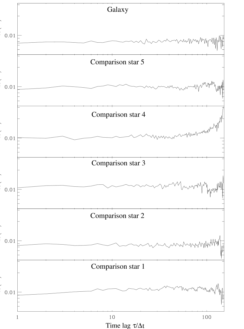
Figure 4: The corresponding structure functions of Mkn 590 and its associated comparisons stars with a temporal sampling $\Delta t\simeq 90$ s. No variability time lag appears.

all cases and often smaller than $0.5\%$ which underlines the precision of the method employed. We consider a galaxy to be variable if firstly $\sigma_{obs}\geq 2\sigma_{ph}$ (i.e. $\sigma_{supp}\geq\sqrt{3}\sigma_{ph}\simeq 2\sigma_{ph}$) and secondly at least one comparison star is stable. From table (2), it appears that we have no clear variability detection for any of the objects of the sample, with some limited cases for Mkn 478, Mkn 684, Mkn 1392 and NGC 4151, studied further. Figure 3 shows the typical light curves obtained by our algorithm for a non-variable (according to the previous criteria) galaxy, Mkn 590, and 5 comparison stars. The corresponding structure functions are also plotted in Fig. 4. They are all flat (the form of the structure function for $\tau\geq 100$ is smarred by large statistical errors not plotted in the graph) meaning that no continuous trend are present in the data during the period of observations. The light curves of each galaxy and the associated comparison stars are plotted in Fig. 7 at the end of this paper.

4.2 Individual objects

We only presents results for the most interesting objects either because they have a limit variability detection or because they have been previously studied by other authors. We develop succinctly some tests used to confirm or not any variability detection.

4.2.1 Mkn 684 and Mkn 1383

These galaxies fulfill the two criteria of variability since $\sigma_{supp}\geq 3\sigma_{ph}$ and their comparison star 2 is non variable. Yet only one comparison star, in each case, has a flat structure function and the other ones increase with time lag. We suspect that a selection effect may occur in our algorithm (see Section 3.2). Thus, we start again the treatment, including the galaxy in the set of comparison stars. All the new structure functions appear finally stable for all time lags, quashing any variability detection.

4.2.2 Mkn 1392

Figure 5: The corresponding structure functions of Mkn 1392 and its associated comparisons stars with a temporal sampling $\Delta t\simeq 300$ s. The structure function of the galaxy increases slightly during the run which may indicate a variability on time scale larger than the length of the observation.

This galaxy fullfills equally the criteria of variability and its structure function increases slightly during the run whereas the comparison star ones are stable (see Fig. 5). This trend remains even if we include the galaxy in the comparison star. It seems, thus, that Mkn 1392 may be variable but on a timescale larger than the length of the observations ($\simeq$ 4 hours).

4.2.3 NGC 4151

As previously said (see Section 3.2.3), important selection effect may exist in the treatment of this galaxy, since there is only one brigth star in the CCD field. To minimize these effects, we repeat the treatment but including the galaxy in the set of comparison stars. The structure function of the galaxy and its diffuse component become stable whereas the star one slightly increases during the run. We have thus to be very carefull when using differential photometry with this galaxy, since the nearest bright star seems to be variable on timescale of hours.

4.3 Infrared observations

Table 3: Same as table 2 but in J band for 3 galaxies of the sample

Name	$\bar{\sigma}_{obs}$	$\bar{\sigma}_{ph}$	$\bar{\sigma}_{supp}$
	(%)	(%)	(%)
Mkn 1392	3.55	1.59	2.30
star1	2.68	0.95	3.49
star2	3.86	2.32	2.40
star3	3.02	1.92	0.90
star4	6.63	3.30	6.05
Mkn 478	5.12	1.59	5.12
star1	2.26	0.62	2.07
star2	6.69	1.95	6.43
Mkn 1098	2.71	1.40	2.30
star1	4.31	1.40	3.80
star2	0.70	1.00	3.50
star3	3.02	2.80	0.60

Three galaxies of the sample, Mkn 478, Mkn 1392 and Mkn 1098, have been observed simutaneously in I and J bands. We treat the J band data with the same algorithm described in Section 3.2. At this wavelength we are clearly limited by the CCD and sky background noises. We can not obtain precision smaller than 2% and it is in the range 2-5 % in most cases. The results are reported in table 3. Only Mkn 478 fulfills the first variability criterium, since all comparison stars seem variable. But, once again, only two comparisons stars were used and a selection effect occurs. No more variability is detected when the galaxy is included in the set of comparison stars.

5 Discussion

The simultaneous observations of NGC 4051 in the IR-optical and X-ray wavebands by Done et al (Don90 (1990)) have given very strong constraints on the spatial distribution of the emitting regions. Effectively, in this object, the limits on the amount of rapid variability in the optical/IR were below 1 and 5 per cent while the X-ray flux continually flickered by up to a factor 2. It clearly rules out models in which the IR/optical and X-ray continuum emission are produced in the same region. Nonetheless, the IR/optical continuum could be the sum of two different components. The first one could originate in the outflows observed in most Seyfert galaxies (Wilson Wil93 (1993), Colbert et al. Col96 (1996)), through synchrotron process on large scale magnetic field. Due to the large sizes of the flows, we expect no rapid variabilities from this emission. On the contrary, a second component, whose flux is noted $F_{syn}$, could be associated with the synchrotron emission of the non-thermal distribution of relativistic electrons producing X-rays, and thus concentrated in a much smaller region. Since rapid X-ray variability is a common features in such objects (Mc Hardy et al. McH85 (1985), Mushotzky et al. Mus93 (1993), Grandi et al. Gra92 (1992)) and is likely associated with instabilities in the source of particles, we expect flickering from this second component too. We assume that its variability amplitude is of the order of the flux, that is $\sigma(F_{syn})\simeq F_{syn}$ which seems reasonable since it is the case in the X-ray range (Mushotzky et al. Mus93 (1993), Ulrich et al. ulr97 (1997)). The treatment allows thus to estimate an upper limit of this variable component by measuring $\sigma_{supp}$ and therefore to constrain the intrinsic properties of the local environment of the emission region. Our assumptions are presented in the following.

5.1 Basic hypotheses

Table 4: Characteristics of 7 galaxies of the sample. The flux density are given in $10^{-11}erg.s^{-1}.cm^{-2}$, lengths in centimeter and magnetic fields in gauss units. Data are taken from Walter & Fink Wal92 (1992). The maximum of $B_{\mbox{\tiny{sup}}}$ gives an absolute upper limit on the magnetic field in the AGN in order not to detect variability.

Name	$F^{\mbox{\tiny{2 keV}}}_{\mbox{\tiny{X}}}$	$F^{\mbox{\tiny{1375 \AA}}}_{\mbox{\tiny{UV}}}$	$F_{\mbox{\tiny{syn}}}$	s	$R_{s}$	$R_{var}$	$max(B_{\mbox{\tiny{sup}}})$
Mkn 359	$0.12\pm 0.01$	$2.76\pm 0.54$	0.03	0.9	8$10^{10}$	-	2.5$10^{5}$
Mkn 590	$1.51\pm 0.22$	$8.36\pm 1.08$	0.01	0.9	6$10^{11}$	-	1.6$10^{4}$
ARK 120	$1.56\pm 0.06$	$22.3\pm 3.3$	0.03	1.1	2$10^{12}$	-	1.9$10^{4}$
MCG+08-11-11	$2.55\pm 0.11$	$1.98\pm 2.46$	0.01	0.7	8$10^{10}$	-	8000
NGC 4051	$0.54\pm 0.03$	$1.66\pm 0.44$	0.17	0.65	6$10^{8}$	9$10^{12}$	4.7$10^{6}$
Mkn 1383	$0.42\pm 0.03$	$11.6\pm 3.9$	0.12	0.9	8$10^{12}$	-	2.4$10^{4}$
Mkn 478	$0.41\pm 0.04$	$7.47\pm 2.04$	0.008	0.9	4$10^{12}$	-	9.0$10^{3}$

We suppose the non-thermal plasma region to be spherical, with radius $R$. As explained above, the particles emit synchrotron radiation in a magnetic field of strength $B$. We also assume the electrons density distribution follows a power law with spectral index $s$, i.e. $\displaystyle n(\gamma)=n_{0}\gamma^{-s}$, with $\gamma_{min}\leq\gamma\leq\gamma_{max}(\gg\gamma_{min})$. If we assume the magnetic field to be uniform throughout the emitting region and with a random direction in the line of sight, the spectral density of the synchrotron flux received by an observer at a distance $D$ away, can be approximated by (Blumenthal & Gould Blu70 (1970)):

$$F_{\nu}^{syn}=\left\{\begin{array}[]{ll}E(s)B^{\frac{s+1}{2}}\frac{n_{0}R^{3}}{D^{2}}\nu^{-\frac{s-1}{2}}&\mbox{if $\nu_{t}<\nu<\nu_{c}$}\\ 0&\mbox{if $\nu_{c}<\nu$}\end{array}\right.$$ (6)

In this equation, $E(s)$ is a function of $s$ solely, $\nu_{c}$ the cut-off frequency of the radiation which depends on the maximum Lorentz factor of the electrons (Blumenthal & Gould Blu70 (1970), Rybicki & Lightman Ryb89 (1989)):

$$\nu_{c}\simeq\frac{3q}{4\pi mc}\gamma_{max}^{2}B.$$ (7)

and $\nu_{t}$ the synchrotron self-absorption frequency separating the optically thin and optically thick regimes of synchrotron emission (see Pacholczyk Pac70 (1970)).
On the other hand, the same electron population produces X-ray radiation by Inverse Compton (IC) process on UV photons, generally supposed to be produced by an accretion disk . We assume that the UV source is roughly at a distance $Z$ from the non-thermal plasma. Finally we suppose that the UV photons density can be approximate by a delta function, and thus, at the location of the hot source, this density can be expressed as follows:

$$n_{\mbox{\tiny{UV}}}(\nu)=\frac{F_{\mbox{\tiny{UV}}}D^{2}}{h\nu_{\mbox{\tiny{UV}}}Z^{2}c}\delta(\nu-\nu_{\mbox{\tiny{UV}}})$$ (8)

where $F_{\mbox{\tiny{UV}}}$ is the observed UV flux. We can then deduced the X-ray flux received by an observer at a distance $D$ away (Blumenthal & Gould Blu70 (1970), Rybicki & Lightman Ryb89 (1989)):

$$F_{\nu}^{\mbox{\tiny{X}}}=F(s)F_{\mbox{\tiny{UV}}}\frac{n_{0}R^{3}}{Z^{2}}\nu_{\mbox{\tiny{UV}}}^{\frac{s-3}{2}}\nu^{-\frac{s-1}{2}}.$$ (9)

where $F(s)$ is solely a function of $s$. This expression is representative of the common spectrum of Seyfert galaxies between 2-10 keV which is well fitted by a power with mean spectral index $s\simeq 2.8$ (Mushotzky et al. Mus93 (1993)).

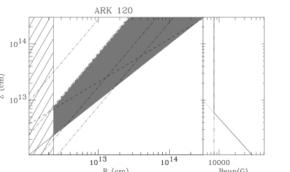
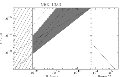
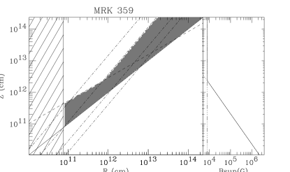
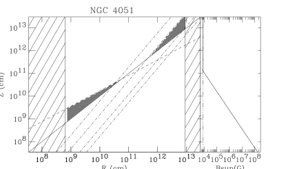
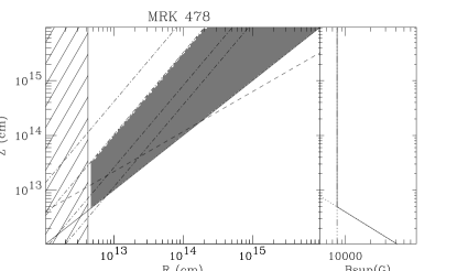
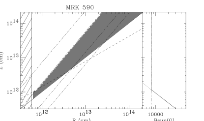
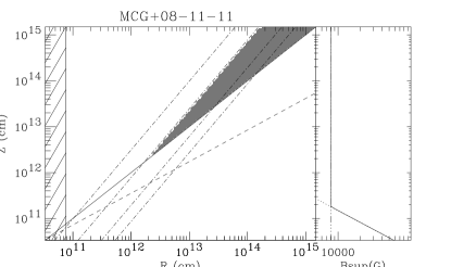
Figure 6: The left part of each plot gives limits on R and Z for 7 galaxies of our sample whose parameters are reported in Table 4. The dash lines represent the equipartition $B_{eq}=B_{\mbox{\tiny{flux}}}$ (Eq. (18)) whereas the set of dot-dash lines represents the equipartition $B_{eq}=B_{\mbox{\tiny{cut-off}}}(\gamma_{max})$ for different values of $\gamma_{max}$ (Eq. (19)). From left to right, $\gamma_{max}$= 50, 100, 200 and 300, corresponding to $B_{eq}\simeq$ 32000 G, 8000 G, 2000 G and 1000 G. Finally, the solid line refers to the $Z=R$ (Eq. (12)). For each galaxy, the allowed region is constrained by Eqs. (10), (11), (12), (18) and (19). It is colored in grey in each plot for $\gamma_{max}=100$. Other $\gamma_{max}$ values would correspond to another dot-dash curve (called type II in the text). The hashed regions are forbidden by Eqs. (10) and (11).
On the right part of each graphic, we have plotted $B_{\mbox{\tiny{sup}}}(Z)$ in solid line. The dot line and three dots-dash line correspond respectively to $B_{\mbox{\tiny{flux}}}(Z)$ and $B_{\mbox{\tiny{cut-off}}}(Z)$. Thus $B_{\mbox{\tiny{sup}}}=B_{\mbox{\tiny{flux}}}(Z)$ when Eq. (18) applied and $B_{\mbox{\tiny{sup}}}=B_{\mbox{\tiny{cut-off}}}(Z)$ when Eq. (19) applied

5.2 Constraint deduced on $R$ and $Z$

First of all, it seems likely that $R\geq R_{s}$, where $R_{s}$ is the Schwarzschild radius of the black hole supposed to power the AGN. We obtain a lower limit for $R_{s}$ through the Eddington limit. Assuming $L_{\mbox{\tiny{UV}}}=4\pi D^{2}F_{\mbox{\tiny{UV}}}$ as roughly equal to the bolometric luminosity, it gives:

$$R\geq R_{s}\geq\frac{L_{\mbox{\tiny{UV}}}\sigma_{t}}{2\pi m_{p}c^{3}}.$$ (10)

On the contrary, the smaller X-ray time variability $\Delta t_{min}$ (if known) gives an upper limit for the size of the non-thermal source:

$$R\leq R_{var}=c\Delta t_{min}.$$ (11)

Finally, we must have at least:

$$Z\geq R.$$ (12)

On the other hand, it appears from Eq. (6) that, to observe no synchrotron emission at the I band frequency $\nu_{\mbox{\tiny{I}}}$, a sufficient (but not necessary) condition is $\nu_{\mbox{\tiny{I}}}\geq\nu_{c}$, that is the upper cut-off of the spectrum lies below our observed frequency. It gives thus a possible upper limit for the strength of the magnetic field:

$$B\leq B_{\mbox{\tiny{cut-off}}}\simeq\frac{4\pi mc}{3q}\frac{\nu_{\mbox{\tiny{I}}}}{\gamma_{max}^{2}}=\frac{C_{\mbox{\tiny{cut-off}}}}{\gamma_{max}^{2}}.$$ (13)

We can also constraint $\gamma_{max}$ since we know that the X-ray spectrum of Seyfert galaxies can be fitted by a power law from $\simeq 1keV$ to $\simeq 100-500\ keV$, where an exponential cut-off is observed (Jourdain et al. Jou92a (1992); Maisack et al. Mais93 (1993); Dermer & Gehrels DermGehr95 (1995)). Since the mean frequency of the soft UV photons is roughly in the range $5-50\ eV$ (Walter et al. Wal94 (1994)), the maximum Lorentz factor $\gamma_{max}$ of the particles must be in the range 50-300.
Besides, limits on $\sigma_{supp}$ resulting from our data analysis (see Section 3) give upper limits on the flux of the variable component $F_{\mbox{\tiny{syn}}}=\nu_{\mbox{\tiny{I}}}F_{\nu}^{syn}$ for each galaxy. Consequently, combining Eqs.(6) and (9) we obtain another possible upper limit for the magnetic field:

$$B\leq B_{\mbox{\tiny{flux}}} = \left(\frac{F(s)}{E(s)}\frac{D^{2}}{Z^{2}}\frac{F_{\mbox{\tiny{syn}}}F_{\mbox{\tiny{UV}}}}{F_{\mbox{\tiny{X}}}}\left(\frac{\nu_{\mbox{\tiny{I}}}\nu_{\mbox{\tiny{UV}}}}{\nu_{\mbox{\tiny{X}}}}\right)^{\frac{s-3}{2}}\right)^{\frac{2}{s+1}}$$ (14)

$$= C_{\mbox{\tiny{flux}}}Z^{-\frac{4}{s+1}}$$

In this equation $\nu_{\mbox{\tiny{X}}}$ is the mean X-ray frequency depending on the X-ray data for each objects, and $F_{\mbox{\tiny{X}}}=\nu_{\mbox{\tiny{X}}}F_{\nu_{\mbox{\tiny{X}}}}^{\mbox{\tiny{X}}}$ is the associated mean flux. Thus, no microvariability detection in any galaxy of our sample, means that:

$$B\leq max(B_{\mbox{\tiny{cut-off}}},\ B_{\mbox{\tiny{flux}}})=B_{sup}.$$ (15)

We have studied these differents constraints for only seven galaxies of our sample whose UV and X-ray luminosity and spectral index are reported in Walter & Fink (Wal93 (1992)). These data are gathered together in Table 4, with the corresponding values of $R_{s}$, $R_{var}$, $F_{\mbox{\tiny{syn}}}$ and $B_{flux}$ for each of the galaxies. The galaxy NGC 4051 is the only one for which a variability in the X-ray is known, down to 100 s. As a conservative value to estimate the maximum X-ray size for this galaxy, we use $\Delta t_{min}$ = 300 s.
Further constraint come from equipartition between particles and magnetic field. Effectively, non-thermal particles need to be accelerated to compensate synchrotron and Inverse Compton losses and magnetic field is generally invoked in the acceleration process (Fermi processes in a shock for example). In this case the magnetic energy density must be equal or larger than the particles energy density. Defining the equipartition value $B_{eq}$ for the magnetic field:

$$\frac{B^{2}_{eq}}{8\pi}=\frac{n_{0}mc^{2}\gamma_{min}^{2-s}}{s-2}$$ (16)

and deducing $n_{0}$ from Eq.(9), we must have finally:

$$B\geq B_{eq} = \left(\frac{8\pi Z^{2}mc^{2}}{(s-2)\gamma_{min}^{2-s}R^{3}F(s)}\frac{F_{\tiny{X}}}{F_{\mbox{\tiny{UV}}}}\left(\frac{\nu_{\tiny{X}}}{\nu_{\mbox{\tiny{UV}}}}\right)^{\frac{s-3}{2}}\right)^{1/2}$$ (17)

$$= C_{eq}\frac{Z}{R^{3/2}}$$

Inequalities (15) and (17) reduce finally to inequalities between $Z$ and $R$:

$$Z\leq\left(\frac{C_{flux}}{C_{eq}}R^{3/2}\right)^{\frac{s+1}{s+5}}\hskip 14.22636pt(\text{corresponding to }B_{eq}\leq B_{flux})$$ (18)

or

$$Z\leq\frac{C_{\mbox{\tiny{cut-off}}}}{C_{eq}}\frac{R^{3/2}}{\gamma_{max}^{2}}\hskip 28.45274pt(\text{corresponding to }B_{eq}\leq B_{cut-off})$$ (19)

Plots Z vs. R of Fig. 6 compiled the constraints described above. We have plotted the curves (type I) corresponding to constraint (18) for each galaxy in dashed line. The second inequality (19) gives a set of limiting curves (type II) on the assumed value of $\gamma_{max}$. Since these curves represent the equipartition $B_{eq}=B_{\mbox{\tiny{cut-off}}}(\gamma_{max})$, they can also be considered as isocontours of $B_{eq}(R,Z)$. We have plotted type II curves corresponding, from left to right, to $\gamma_{max}=50,\ 100,\ 200,\ 300$, which correspond to $B_{eq}=32000\ G,\ 8000\ G,\ 2000\ G$ and $1000\ G$. The diagrams must be read as follows:

1. For each galaxy, the allowed region is constrained by Eqs. (10), (11), (12), (18) and (19). It is colored in grey in each plot for $\gamma_{max}=100$. Other $\gamma_{max}$ values would correspond to another curve of type II. The hashed regions are forbidden by Eqs. (10) and (11).

2. At a given point inside the allowed region, a lower limit of $B$ is given by $B_{\mbox{\tiny{eq}}}$, represented by the type II curve passing through this point. An upper limit is given by $B_{\mbox{\tiny{flux}}}$ if Eq. (18) applies or by $B_{\mbox{\tiny{cut-off}}}$ if Eq. (19) applies. $B_{\mbox{\tiny{flux}}}$, $B_{\mbox{\tiny{cut-off}}}$ and $B_{\mbox{\tiny{sup}}}$ are plotted on the right of each graphic. The equality $B_{\mbox{\tiny{flux}}}=B_{\mbox{\tiny{cut-off}}}$ is realized, for a given assumed value of $\gamma_{max}$, when type I and type II curves intersect. An absolute maximum of the magnetic field is obtained for the smaller value of $Z$ in the allowed region. This value is also reported in Table 4.

An allowed region exists for each galaxy, with a critical case for NGC 4051, where the space parameter is strongly constrained. However our results for this galaxy disagree with those of Celotti et al. (Cel91 (1991)), since if we assume, like them, that the size of the X-ray region is strictly equal to $R_{var}$, we are intside the allowed region for non-thermal models. But these results need to be used with care, in the case of this galaxy, since it seems unlikely for R and Z to be so fine tuned. These different results are obviously affected by the lack of simultaneous X-ray and Optical-UV data and constraints could be tightened if rapid X-ray variability were detected for most of these objects. It appears however that non-thermal model can not be ruled out by our data and can still explain the high energy spectra of Seyfert galaxies.

6 Conclusion

Upper limits on optical microvariabilities in a large sample of 22 Seyfert galaxies have been obtained, using differential photometry. We have developped a new method of analysis minimizing the influence of possible variability of the comparison stars. We thus obtain precision on our variability detection smaller than 1% and in most cases about 0.5%. We do not detect variability in any of our objects, with a possible trend of several hours in Mkn 359. In the hypothesis where variable optical emission would be due to synchrotron radiation from the non-thermal electron population which we suppose to be responsible for the X-ray emission, these results enable us to constraint intrinsic properties of the local environment of the non thermal source. Upper limits on our variability detection and equipartition hypothesis between magnetic field and particle, restrain the possible values of the size R of the non thermal source, its distance Z from the UV emission region and fix upper and lower limits for the magnetic field.

Acknowlegements: We are grateful to the referee, Prof. Gopal Krishna, for his precious comments and really careful reading of the manuscript. We feel that his suggestions and criticisms have certainly improved this paper.

Figure 7: Light curves of the different galaxies and associated comparison stars of the sample.

Figure 7: To be continued.

Figure 7: To be continued.

Figure 7: To be continued.

Figure 7: To be continued.

Figure 7: To be continued.

References

- (1) Aslanov A. A., Kolosov, D. E., Lipunova, N. A., et al., 1989, SvAL 15, 132
- (2) Barr P., Willis A.J., Wilson R., 1983, MNRAS 203, 201
- (3) Blumenthal G. R., Gould R. J., 1970, Rev. Mod. Phys. 42, 237
- (4) Carini, M. T. 1990, The time scales of the optical variability of blazars, Ph.D. Thesis, 11
- (5) Carini, M. T., et al., 1991, AJ 101, 1196
- (6) Carini, M. T., Miller, H. R., Noble, J. C., et al., 1992, AJ 104, 15
- (7) Celotti, A., Ghisellini, G., Fabian A. C., 1991, MNRAS 251, 529
- (8) Chakrabarti S. K. & Wiita P. J., 1993, ApJ 411, 602
- (9) Colbert, E. J. M., Baum, S. A., Gallimore, J. F., O’Dea, C. P., & Christensen, J. A. 1996, ApJ 467, 551
- (10) Cruz-Gonzàlez, I., Carrasco, L., Ruiz, E., et al., 1993, Rev. Mex. Astron. Astrof. 29, 197
- (11) Dermer C.D., Gehrels N., 1995, ApJ 447, 103
- (12) Done C., Ward M. J., Fabian A. C., et al., 1990, MNRAS 243, 713
- (13) Doroshenko, V. T., Lyutyĭ V. M., Sillanpää, A., Valtaoja, E., 1992, in Variability of Blazars, eds. E. Valtaoja & M. Valtonen (Cambridge: University Press), p. 358
- (14) Dultzin-Hacyan, D., Schuster, W., Parrao, L., et al., 1992, AJ 103, 1769
- (15) Dultzin-Hacyan,, Ruelas-Mayorga, A., Costero, R., 1993, Rev. Mex. Astron. Astrof. 25, 143
- (16) Ginzburg V. L. and Syrovatskii S. I., 1965, ARAA 3, 297
- (17) Gopal-Krishna, Ram Sagar, Wiita P. J., 1995, MNRAS 274, 701
- (18) Gopal-Krishna, Wiita P. J., 1992, A&A 259,109
- (19) Gopal-Krishna, Ram Sagar, Wiita P. J., 1993, MNRAS 262, 969
- (20) Grandi, P., Tagliaferri, G., Giommi, P., Barr, P., & Palumbo, G. G. C. 1992, ApJS, 82, 93
- (21) Haardt F. & Maraschi L., 1991, ApJ 380, 51
- (22) Henri G. & Petrucci P. O., 1997, A&A 326, 87
- (23) Hunt, L. K., Mannucci, F., Salvati, M., & Stanga, R. M. 1992, A&A, 257, 434
- (24) Jang M. & Miller H. R., 1995, ApJ 452, 582
- (25) Jang M. & Miller H. R., 1997, AJ 114 (2), 565
- (26) Jourdain E., et al., 1992a, A&A 256, L38
- (27) Koenig M., Staubert R., Wilms J., 1997, A&A 326, L25
- (28) Landolt A. U., 1992, AJ 104, 340
- (29) Lyutyĭ V. M., Doroshenko, V. T., 1993, SvAL 19, 405
- (30) Lyutyĭ V. M., Aslanov A. A., Khruuzina T. S., et al., 1989, SvAL 15, 247
- (31) Lawrence A., Giles A. B., Mc Hardy I. M. and Cooke B. A., 1981, MNRAS 195, 149
- (32) Malaguti G., Bassani L., Caroli E., 1994, ApJS 94, 517
- (33) McHardy I., 1985, SSRv 40, 559
- (34) Maisack M., et al., 1993, ApJ 407, L61
- (35) Mangalam A. V., Wiita P. J., 1993, ApJ 406,420
- (36) Miller H. R., Carini M. T., Noble J. C., Webb J. C., Wiita P. J., 1992, in Variability of Blazars, eds. E. Valtaoja & M. Valtonen (Cambridge: University Press), p. 320
- (37) Mushotzky, R. F., Done, C., & Pounds, K. A. 1993,, ARAA 31, 717
- (38) Paltani S. et al., 1997, A&A 327, 539
- (39) Pacholczyk, A. G. 1970, Radio Astrophysics (W. H. Freeman: San Francisco)
- (40) Qian S. J., Quirrenbach A., Witzel A., et al., 1991, A&A 241, 15
- (41) Véron-Cetty M.-P., Véron P., 1989, ESO Sci. Rep. No. 13
- (42) Rabette 1998, A&AS, in press
- (43) Rutman J., 1978, Proc. IEEE 66, 1048
- (44) Rybicki, G., B. & Lightman, A., P., 1979, in Radiative processes in Astrophysics, Wiley-interscience, New-York.
- (45) Simonetti J.H., Cordes J.M. & Heeschen D.S., 1985, ApJ 296, 46
- (46) Ulrich, M. H., Maraschi, L., Megan, C., 1997, ARA&A 35, 445
- (47) Wagner S., 1992, in Variability of Blazars, eds. E. Valtaoja & M. Valtonen (Cambridge: University Press), p. 346
- (48) Walter R. & Courvoisier T. J.-L., 1992, A&A 266, 65-71
- (49) Walter R. & Fink H. H., 1993, A&A 274, 105
- (50) Walter et al., 1994, A&A 285, 119
- (51) Wiita P. J., Miller H. R., Carini M. T., Rosen A., 1991, in structure and Emission Properties of Accretion, IAU Colloquium No. 129, edited by J. P. Lasota et al. (Editions Frontieres, Gif sur Yvette), p. 557
- (52) Wiita P. J., Miller H. R., Gupta N., Chakrabarti S. K., 1992, in Variability of Blazars, eds. E. Valtaoja & M. Valtonen (Cambridge: University Press), p. 311
- (53) Wilson, A. S. 1993, in Astrophysical Jets, ed. D. Burgarella, M. Livio & C.P. O’Dea (Cambridge: Cambridge Univ. Press), 121
- (54) Zdziarski, A. A., Fabian, A. C., Nandra, K., 1994 MNRAS 269, L55