A transition from linear to circular polarization in pulsar radio emission

Abstract

At present three pulsars are known which clearly show a strongly increasing degree of circular polarization with frequency. As this is accompanied by a smooth decrease of linear polarization, we investigate, if this observation can be explained through a propagation mode transition from linear to circular polarization. Using a previously published model we find that the rate of change of the polarization types with frequency is well consistent with the theory.

The small number of only three objects does of course not allow to draw a general conclusion for the whole sample of pulsars. However we show that the very unusual behavior of these three objects can be well explained with this model and we discuss, why only so few such objects are presently known.

1 Introduction

Whether the observed polarimetric features of pulsar radio emission are intrinsic properties of the emission mechanism or if they are a result of propagational effects is one of the open questions for the understanding of the polarization of radio pulsars. Early observations of the ‘S’-type swing of the polarization position angle through the pulse profile of the Vela pulsar led to an geometrical interpretation by Radhakrishnan & Cooke (1969). In their model the swing reflects the geometry of the magnetic field lines projected on the plane of the sky. In some cases the expected swing is matched so well that a non-geometrical origin for the position angle seems rather improbable. Ruderman & Sutherland (1975) gave an explanation for this phenomenon as an intrinsic property of emission by coherent curvature radiation. The particles experience an acceleration perpendicular to their motion in the plane of curvature of the field line. The resulting radiation has its electric field vector within this plane, thus producing the geometrical signature.

Alternatively, it was proposed that the observed polarization originates from propagational effects or is at least influenced by them. Various authors calculated the properties of the propagational modes in a pulsar magnetosphere (e.g. Allan & Melrose 1982, Barnard & Arons 1986, Lyutikov 1998 and references therein). It is widely agreed among those authors, that two independent, generally elliptical polarization modes propagate, which are oriented parallel and perpendicular to the plane of curvature of the magnetic field line. The observed polarization then corresponds to the shape of these modes at the distance from the neutron star, where the radiation decouples from the plasma. This distance is called the polarization limiting radius (hereafter PLR) and does not necessarily coincide with the place of emission. The magnitude of the PLR has been a subject of theoretical debates. Barnard (1986) and Beskin et al. (1993) place the PLR at the cyclotron resonance. Melrose (1979) defines a coupling ratio $Q=1/(\Delta kL)$ where $\Delta k$ denotes the difference in wavenumber of the two modes and $L$ is a characteristic length scale. The PLR is at the position where $Q\simeq 1$.

In a previous paper (von Hoensbroech et al. 1998b) we have shown that many of the complex variety of radio pulsar polarization states can be understood qualitatively if some propagational effects in the pulsar magnetosphere are taken into account. This was done by using a simple approximation for the properties of natural polarization modes as they propagate through the magnetosphere. The model is based on the following assumptions: 1. The temperature of the background plasma is assumed to be zero (distribution function $f(\gamma)=\delta(\gamma-\gamma_{\rm bg})$, hereafter $\gamma_{\rm bg}$ is the $\gamma$-factor of the background plasma). 2. Furthermore no strong pair production in a sense, that the $e^{-}e^{+}$-plasma is not approximately neutral, is assumed. Considering all relevant angles under which the propagating wave and the magnetic field lines intersect, the shape of the natural polarization modes can be calculated at any given point between the emission height and the light cylinder radius (hereafter $R_{\rm LC}$, $R_{\rm LC}=cP/2\pi$). 3. Assuming a PLR and a certain Lorentz-factor for the background plasma, the following qualitative statements can be made: a. The polarization modes propagate independently with their position angle parallel and orthogonal to the local plane of field line curvature, b. the radiation depolarizes towards high frequencies, c. the degree of polarization correlates with the pulsars loss of rotational energy $\dot{E}$ and d. the polarization smoothly changes from linear to circular with increasing frequency.

This last point was met by recent observations at the relatively high radio frequencies of $\nu_{\rm obs}=4.9$ GHz (von Hoensbroech et al. 1998a) as it was already suspected by early measurements of Morris et al. (1981). For a few pulsars the degree of circular polarization increases strongly with frequency. For three of those objects, the circular polarization reaches values of more than 50 %, even surpassing the linear polarization. This rather unusual behavior appears smooth and is thus likely to be systematic, as an inspection of lower frequency data showed. We therefore use the data of those three clear examples to quantitatively compare the rate of change from linear to circular to the predicted one in statement d.

2 Analysis and Results

Figure 1: Position of the three pulsars in the $P-\dot{P}$–diagram for which the change from linear to circular polarization has been observed. They do not form a coherent group within the pulsar sample. One of them is very young, one is rather average and the third one is a relatively old object.

Table 1: Polarization data and references for all three pulsars.

Pulsar	Freq. [MHz]	$\Pi_{\rm L}$[%]	$\Pi_{\rm C}[\%]$	$R$	Ref.
B0144+59	610	$29\pm 2$	$11\pm 3$	$2.64\pm 0.74$	[1]
	1408	$23\pm 1$	$24\pm 2$	$0.96\pm 0.09$	[1]
	1642	$25\pm 6$	$26\pm 6$	$0.96\pm 0.32$	[1]
	2695	$16\pm 3$	$50\pm 4$	$0.32\pm 0.07$	[4]
	4850	$12\pm 1$	$50\pm 2$	$0.24\pm 0.02$	[2]
B1737$-$30	610	$22\pm 1$	$20\pm 1$	$1.10\pm 0.07$	[1]
	660	$43\pm 3$	$17\pm 4$	$2.53\pm 0.62$	[3]
	925	$73\pm 2$	$21\pm 2$	$3.48\pm 0.34$	[1]
	1408	$80\pm 1$	$38\pm 1$	$2.11\pm 0.06$	[1]
	1642	$71\pm 1$	$45\pm 1$	$1.58\pm 0.04$	[1]
	4750	$53\pm 7$	$59\pm 5$	$0.90\pm 0.14$	[2]
B1913+10	408	$18\pm 2$	$13\pm 3$	$1.38\pm 0.35$	[1]
	610	$38\pm 2$	$22\pm 2$	$1.73\pm 0.18$	[1]
	925	$77\pm 4$	$35\pm 3$	$2.20\pm 0.22$	[1]
	1408	$50\pm 1$	$42\pm 1$	$1.19\pm 0.04$	[1]
	1642	$49\pm 2$	$46\pm 3$	$1.07\pm 0.08$	[1]
	4850	$21\pm 4$	$55\pm 5$	$0.38\pm 0.08$	[2]

Presently we have data for three pulsars, where a clear change from linear to circular polarization towards high frequencies is observed (see Fig. 5 in von Hoensbroech et al. 1998b). It is obvious from Fig. 1 that the three objects have very different rotational periods $P$ and period time derivatives $\dot{P}$. Hence they do not form an isolated group with respect to their rotational parameters. Since the change from linear to circular polarization is superposed by general depolarization effects, which affect both types of polarization likewise, the degrees of polarization cannot be compared directly with the theory. Therefore we choose the ratio

$$R:=\frac{\Pi_{L}}{\Pi_{C}}$$ (1)

between the degrees of linear ($\Pi_{L}$) and the circular ($\Pi_{C}$) polarization as an depolarization independent parameter. $R$ and its statistical error $\Delta R$ can easily be calculated from the data.

The polarization data we used for this analysis were accessed through the online EPN-database (http://www.mpifr-bonn.mpg.de/pulsar/data/). The calibrated data were extracted in the EPN-format (Lorimer et al. 1998). The degrees of polarization were calculated using the same routine for all profiles. All relevant parameters and references are listed in Table 1.

The theoretical functional dependence of $R$ can be derived from equation (25) in (von Hoensbroech et al. 1998b). Applying a Taylor-expansion in inverse frequency $\nu^{-1}$ to the first order yields

$$R(\nu) = \frac{\Omega_{e,{\rm PLR}}}{\gamma_{\rm bg}}\frac{\sin^{2}\theta_{\rm PLR}}{4\pi(\cos\theta_{\rm PLR}-\beta)(1-\beta\cos\theta_{\rm PLR})^{2}}\cdot\nu^{-1}$$ (3)

$$+O\left(\nu^{-3}\right)\ .$$

Here $\Omega_{e,{\rm PLR}}$ is the local electron gyro frequency at the PLR, $\theta_{\rm PLR}$ the angle between the propagating wave and the direction of the local magnetic field at the PLR and $\beta=v/c=\sqrt{1-1/\gamma_{\rm bg}^{2}}$ the streaming velocity of the plasma. Higher order terms can be neglected as long as the wave frequency is different from $\sim\Omega_{e}/2\pi$.

Obviously, a $\nu^{-1}$–frequency dependence of $R$ is required by the theory. A comparison of the observed frequency dependence of $R$ with the predicted one is therefore a strong test for the theory. Figs. 2 – 4 show a comparison of the data points and the theoretical curve (dashed line) for $R$.

There are a couple of parameters which indirectly enter Eq. (3) as scaling factors. $\Omega_{e,{\rm PLR}}$ is proportional to the local magnetic field strength $B(PLR)$. This value again depends on basic pulsar parameters such as the period, its time derivative and, if known, on the inclination angle between the rotation- and the magnetic dipole axis. Furthermore the angle $\theta_{\rm PLR}$ between the propagating wave and the local magnetic field depends on the chosen field line and the assumed emission height. For the background plasma Lorentz factor we made the assumption $\gamma_{\rm bg}=200$. Finally we chose the PLR at 20 % of $R_{\rm LC}$. As the values of the PLR and the emission height (2 % of $R_{\rm LC}$ are given as fractions of $R_{\rm LC}$, their absolute values depend on the period. The combination of $\gamma_{\rm bg}$ and PLR was chosen without restriction of generality as various other combinations yield the same result (see Fig. 5).

However, apart from the known intrinsic pulsar parameters $P$ and $\dot{P}$, the same set of parameters was used for all three pulsars. Please note that these parameters only enter Eq. (3) as scaling factors, yielding a parallel displacement of the function. Hence they determine the frequency range where the transition from linear to circular polarization takes place, but not the functional dependence $\sim\nu^{-1}$.

Figure 2: PSR B0144+59, $R=\Pi_{L}/\Pi_{C}$ versus frequency. The theoretical change of $R$ (dashed line) is compared to measured data. The horizontal dotted line corresponds to $R=1$, i.e. linear and circular polarization are of equal strength (here $R=1$ at $\nu=1.4$ GHz). Parameters for theoretical line: $\gamma_{\rm bg}=200,{\rm PLR}=20\%$ of $R_{\rm LC}$.

Figure 3: PSR B1737$-$30, see caption of Fig. 2 and text for details (here $R=1$ at $\nu=3.5$ GHz). See text about the two “outriders’. Parameters for theoretical line: $\gamma_{\rm bg}=200,{\rm PLR}=20\%$ of $R_{\rm LC}$.

Figure 4: PSR B1913+10, see caption of Fig. 2 and text for details (here $R=1$ at $\nu=1.8$ GHz). Parameters for theoretical line: $\gamma_{\rm bg}=200,{\rm PLR}=20\%$

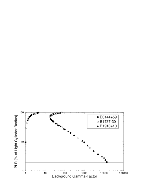
Figure 5: Possible combinations of PLR and $\gamma_{\rm bg}$ which yield consistent results for the prefactor in Eq. (3) which fit to the observed data of each pulsar. A variation of this factor results into a parallel displacement of the theoretical curves in Figs. 2-4. The solid line below corresponds to the assumed emission height at 2 % of the $R_{\rm LC}$ as the minimum PLR.

2.1 PSR B0144+59

This pulsar is the first one in which we found the effect of increasing circular polarization to high frequencies. Its rotational parameters are $P=196$ ms and $\dot{P}=0.3\times 10^{-15}$, yielding to a weak surface magnetic field of ‘only’ $B_{0}=2.3\times 10^{7}$ T, an average value for $\dot{E}=1.3\times 10^{26}$ W and the characteristic age $\tau=1.2\times 10^{7}$ yrs. Reasonable data in full polarization was available between 610 MHz and 4.85 GHz.

Fig. 2 shows the measured values and the theoretical curve for the change of $R$ with frequency.

2.2 PSR B1737$-$30

PSR B1737$-$30 has a spin period of $P=607$ ms and a period derivative of $\dot{P}=466\times 10^{-15}$. The resulting spin down energy loss $\dot{E}=8.3\times 10^{27}W$ places it amongst the top 10% of the pulsar sample. The very low characteristic age $\tau=2\times 10^{4}$ yrs and the very high surface magnetic field $B_{0}=1.7\times 10^{9}$ T make this one an extreme object. Note that in terms of the surface magnetic field, this object is at the opposite end of the “normal” pulsar sample compared to PSR B0144+59.

The change of $R$ with frequency is shown in Fig. 3. Although the two low frequency points do not fit the theoretical function, the frequency change of $R$ smoothly follows this function at higher frequencies. Note that the two outrider profiles are significantly affected by interstellar scattering which could also alter the polarization state when emission from different pulse phases with different polarization states are superposed (see also Sect. 2.4).

2.3 PSR B1913+10

With a spin period $P=405$ ms and its temporal derivative $\dot{P}=15\times 10^{-15}$ this is an average pulsar. This is also reflected by its parameters $\dot{E}=9\times 10^{26}$ W, $B_{0}=2.5\times 10^{8}$ T and $\tau=4\times 10^{5}$ yrs.

Fig. 4 shows the measured values for $R$ and the theoretical function . As for PSR B1737$-$30 the lower frequency points are too small, but at higher frequencies the theoretical curve is matched perfectly. As for the previous pulsar, the two outrider profiles are significantly scattered.

2.4 Outriders

The systematic deviation of the low frequency points is certainly a draw back of these observations. However they can be understood through the following argument: von Hoensbroech et al. (1998a) have shown that the polarization properties in general are much less systematic at low radio frequencies compared to higher ones. This indicates that the polarization of pulsars undergo some sort of randomization at low radio frequencies. This can be caused either through intrinsic variations – e.g. non constant PLR at low frequencies – or through additional propagation effects in the highly magnetized medium close to the pulsar, which mainly affect low radio frequencies.

3 Discussion

Based on a simple propagational scenario for natural polarization modes in pulsar magnetospheres we were able to show that for the available data set of three pulsars, theory and observations are in very good agreement. In these objects the polarization changes smoothly from linear to circular with increasing frequency. The principal theoretical $\nu^{-1}$-functional dependence of of this change, expressed in Eq. (3) is independent of all pulsar parameters (as long as a mono-energetic background plasma is concerned). The individual pulsar parameters enter Eq. (3) only as scaling factors, hence yielding a parallel displacement of the function. Thus the comparison of the calculated and observed functional dependence is a strong test for the theory. As shown in Sect. 2 the rate of change of $R$ with frequency is consistent with Eq. (3).

We note that for all three pulsars the same combinations of $\gamma_{\rm bg}$ and PLR result into quantitative agreements between the measured points and the theoretical curve, although these objects are very different in their parameters $P$ and $\dot{P}$. Obviously not only the $\nu^{-1}$ dependence is in agreement with the observation, but also the scaling of the function as it is defined through the prefactor in Eq. (3) for these three pulsars. This scaling coincidence is remarkable but does not necessarily mean, that all pulsars have to scale in the same manner.

Of course the number of pulsars which clearly show this effect is too small to make a statistically rigorous statement. This is especially true as it cannot be predicted at which frequency this effect should occur and hence for which other pulsars we should have observed it. We emphasize that it is rather difficult to observe such a frequency behavior of polarization since it requires a significant increase of the circular polarization to result into some decrease of the linear because they are added in quadrature.

Pulsars exhibit steep radio spectra, a fact which reduces the total number of available profiles in full polarization to about 100 at 4.9 GHz with many of them at a fairly low signal-to-noise ratio. As pulsars are also known to depolarize towards high frequencies, the signal-to-noise-ratio of the polarized emission is often very low, hardly allowing a credible determination of the ratio between linear and circular polarization. Nevertheless, it has been shown at low frequencies that the linear polarization reduces with frequency while such a trend is not evident for circular polarization (e.g. Han et al. 1998). This result qualitatively fits into the same trend of changing the ratio between the two polarizations. Taking all points mentioned above into account we are not surprised that only three pulsars have been found yet which clearly show this effect and allow an opportunity to test the theory.

In this paper we have used the frequency dependence of integrated profiles. These integrated profiles of course differ strongly from the individual pulses. It has been shown e.g. by Stinebring et al. (1984), that these individual pulses are often highly circularly polarized also at low frequencies. This is not necessarily in contradiction to the ideas described in this paper as the conditions within the magnetosphere are known to be highly non-stationary and unstable. The location at which the radiation decouples from the plasma (PLR) might therefore vary strongly from pulse to pulse. However, the integrated profile represents an average over these individual pulses, corresponding to an average PLR. A crucial test whether the described effect is responsible for the circular polarization would be the simultaneous observation of single pulses in full polarization over large frequency intervals.

Summarizing, we may say that the observations of the three objects support the theoretical approach that the polarization characteristics – and especially the high frequency occurrence of strong circular polarization – of at least these three pulsars are explainable in terms of propagating natural wave modes in the magnetosphere. Thus, it may be worth to follow that line of thought from the theoretical point of view and to try to get some more high quality data of the general polarization properties at low and high radio frequencies.