Deciphering Cosmological Information
from Redshift Surveys of High-$z$ Objects

1 Introduction

Galaxy redshift surveys in 1980s revealed and established the existence of large-scale structure[1] extending around $\sim 100$Mpc in the current universe at $z=0$. Theoretically, many cosmological models are known to be more or less successful in reproducing the structure at redshift $z\sim 0$. In fact, however, this may be largely because there are still several degrees of freedom or cosmological parameters needed to appropriately fit the observations at $z\sim 0$, including the density parameter, $\mathchar 28938\relax_{0}$, the mass fluctuation amplitude at the top-hat window radius of $8{\hbox{$h^{-1}$}{\rm Mpc}}$, $\sigma_{8}$, the Hubble constant in units of $100$km/sec/Mpc, $h$, and even the cosmological constant $\lambda_{0}$. This kind of degeneracy in cosmological parameters among viable models can be broken by combining the data at higher $z$.

With the on-going redshift surveys of millions of galaxies and quasars and with large telescopes with high spectral resolution, one can probe directly the epoch of galaxy formation. One of the most important goals of cosmology in the next century is to construct a physical model of galaxy formation and evolution in the observationally determined cosmological context. To this time this process has been simply parameterized by the notorious bias parameter $b$, whatever its meaning might be. Presently, many theoretical and observational attempts are in progress to replace the parameter $b$ by another physical model. Naturally, observational explorations of the larger-scale structure at $z=0$ and higher redshifts provide important clues to understanding the origin of structure in the universe.

Redshift surveys of galaxies definitely serve as the central database for observational cosmology. In addition to the existing catalogues including CfA1, CfA2, SSRS, and the Las Campanas survey, upcoming surveys such as 2dF and SDSS are expected to provide important clues to our universe. In addition to those shallower surveys, clustering in the universe in the range $z=1-3$ has been partially revealed by, for instance, the Lyman-break galaxies[2] and X-ray selected AGNs.[3]  In particular, the 2dF[4] (2-degree Field Survey) and SDSS (Sloan Digital Sky Survey) QSO redshift surveys promise to extend the observable scale of the universe by an order of magnitude, up to a few Gpc. A proper interpretation of such redshift surveys in terms of the clustering evolution, however, requires an understanding of many cosmological effects which can be neglected and thus have not been considered seriously in redshift surveys of $z\ll 1$ objects.

This paper consists of two topics which should play key roles in the theoretical interpretation of the future redshift surveys of high-redshift objects, the cosmological light-cone effect (§2) and redshift-space distortion (§3). Primarily, we intend to review and describe the two effects in a systematic and comprehensive manner on the basis of several of our papers.[5]${}^{\hbox{\,-}}$[8]  In addition, however, we input new materials in §3.4 and §3.5. Also, §2.2 presents theoretical predictions based on a different bias model from that adopted in one of our previous studies.[5]

In this spirit, the remainder of this paper is organized as follows. Section 2.1 briefly outlines a theoretical formulation of the two-point correlation function on the light-cone hypersurface, following Ref. ?. The corresponding theoretical predictions are presented in Section 2.2 with future QSO redshift surveys in mind. The predictions are based on a different model for evolution of bias from that adopted in Ref. ?. Thus they illustrate the extent to which the effect of bias changes the observable clustering of high-redshift objects. Section 2.3 summarizes the light-cone effect on the higher-order clustering statistics following Ref. ?. Section 3 starts with the basic idea of the cosmological redshift-space distortion (§3.1) and its formulation in linear theory, both of which are on the basis of Ref. ?. Then we comment on the systematic bias in estimating the cosmological parameter from shallower ($z\lower 2.15277pt\hbox{$\;\buildrel<\over{\sim}\;$}0.2$) galaxy redshift surveys, following Ref. ?. The next two subsections are entirely new; Section 3.4 considers uncertainties due to the distance formulae in inhomogeneous cosmological models and to the evolution model of bias, and Section 3.5 examines the feasibility of the cosmological redshift-space distortion as a cosmological test to probe $\mathchar 28938\relax_{0}$ and $\lambda_{0}$. In the latter we fully explore the nonlinear effects also using high-resolution $N$-body simulations. Finally, we summarize the main conclusions in Section 4.

2 Cosmological light-cone effect

Observing a distant patch of the universe is equivalent to observing the past. Due to the finite light velocity, a line-of-sight direction of a redshift survey is along the time, as well as spatial, coordinate axis. Therefore the entire sample does not consist of objects on a constant-time hypersurface, but rather on a light-cone, i.e., a null hypersurface defined by observers at $z=0$. This implies that many properties of the objects change across the depth of the survey volume, including the mean density, the amplitude of spatial clustering of dark matter, the bias of luminous objects with respect to mass, and the intrinsic evolution of the absolute magnitude and spectral energy distribution. These aspects should be properly taken into account in order to extract cosmological information from observed samples of redshift surveys.

For the CfA galaxy survey,[1] for instance, the survey depth extends up to a recession velocity of 15000 km/s, which is interpreted as either $d_{\rm max}=150{\hbox{$h^{-1}$}{\rm Mpc}}$ in spatial distance or $z_{\rm max}=0.05$ in time difference. This translates to a $\sim 10$% difference in the amplitude of $\xi$ and $P(k)$ in linear theory. Compared with the statistical error of the available sample, this level of systematic effect is negligible. Thus it is quite common to compare the observed $\xi$ with the theoretical predictions at $z=0$. The situation will be entirely different for the upcoming galaxy and QSO redshift surveys, 2dF and SDSS; $0.3-1$ million galaxies up to $z_{\rm max}=0.2$, and $0.3-1\times 10^{5}$ QSOs up to $z_{\rm max}=3-5$. Such observational samples motivate us to formulate a theory to describe the clustering statistics, fully incorporating the light-cone effect. In the remainder of this section, we present theoretical predictions for two-point[5] and higher-order correlation[6] functions which are properly defined on the light-cone.

2.1 Defining two-point correlation functions on a light-cone

In this subsection, we derive an expression for the two-point correlation function on the light-cone hypersurface in the spatially-flat Friedmann – Robertson – Walker space-time for simplicity; the line element is given in terms of the conformal time $\eta$ as

$$ds^{2}=a^{2}(\eta)\left[-d\eta^{2}+dr^{2}+r^{2}d\mathchar 28938\relax^{2}\right].$$ (2.1)

Since our fiducial observer is located at the origin of the coordinates ($\eta=\eta_{0}$, $r=0$), an object at $r$ and $\eta$ on the light-cone hypersurface satisfies the simple relation $r=\eta_{0}-\eta$.

We denote the comoving number density of observed objects (galaxies or QSOs satisfying the selection criteria) at $\eta$ and ${\bf x}=(r,{\vec{\gamma}})$ by $n(\eta,{\bf x})$. Then the corresponding number density defined on the light-cone is written as

$${n^{\rm LC}}(r,{\vec{\gamma}})=n(\eta_{0}-r,r,{\vec{\gamma}}).$$ (2.2)

If we introduce the mean observed number density (comoving) and the density fluctuation at $\eta$, $n_{0}(\eta)$ and $\mathchar 28929\relax(\eta,{\bf x})$, on the constant-time hypersurface,

$$n(\eta,{\bf x})=n_{0}(\eta)\left[1+\mathchar 28929\relax(\eta,{\bf x})\right],$$ (2.3)

Eq. (2.2) can be rewritten as

$${n^{\rm LC}}(r,{\vec{\gamma}})=n_{0}(\eta_{0}-r)\left[1+\mathchar 28929\relax(\eta_{0}-r,r,{\vec{\gamma}})\right].$$ (2.4)

The observed number density $n_{0}(\eta)$ is different from the true density of the objects $\overline{n}(\eta)$ at $\eta$ by a factor of the selection function $\phi(\eta)$:

$$n_{0}(\eta)=\overline{n}(\eta)\phi(\eta).$$ (2.5)

Thus $n_{0}(\eta)$ already includes the selection criteria, which depend on the luminosity function of the objects and thus the magnitude-limit of the survey, for instance:

When ${n^{\rm LC}}(r,{\vec{\gamma}})$ is given, one may compute the following two-point statistics:

$${\cal X}(R) = {1\over V^{\rm LC}}\int{d\mathchar 28938\relax_{\hat{\bf R}}\over 4\pi}\int r_{1}^{2}dr_{1}d\mathchar 28938\relax_{{\vec{\gamma}}_{1}}\int r_{2}^{2}dr_{2}d\mathchar 28938\relax_{{\vec{\gamma}}_{2}}$$ (2.6)

$$\times {n^{\rm LC}}(r_{1},{\vec{\gamma}}_{1}){n^{\rm LC}}(r_{2},{\vec{\gamma}}_{2})\delta^{(3)}({\bf x}_{1}-{\bf x}_{2}-{\bf R}).$$

Here ${\bf x}_{1}=(r_{1},r_{1}{\vec{\gamma}}_{1})$, ${\bf x}_{2}=(r_{2},r_{2}{\vec{\gamma}}_{2})$, $R=|{\bf R}|$, $\hat{\bf R}={\bf R}/R$, and $V^{\rm LC}$ is the comoving survey volume of the data catalogue:

$$V^{\rm LC}=\int_{r_{\rm min}}^{r_{\rm max}}r^{2}dr\int d\mathchar 28938\relax_{\vec{\gamma}}={4\pi\over 3}({r_{\rm max}}^{3}-{r_{\rm min}}^{3}),$$ (2.7)

with ${r_{\rm max}}=r(z_{\rm max})$ and ${r_{\rm min}}=r(z_{\rm min})$ the boundaries of the survey volume. Although the second equality as well as the analysis below assumes that the survey volume extends to $4\pi$ steradian, all the results below can be easily generalized to the case of the finite angular extent.

Substituting Eq. (2.4), the ensemble average of an estimator ${\cal X}(R)$ can be explicitly written as

$$\bigl{<}{\cal X}(R)\bigr{>}={\cal W}(R)+{\cal U}(R),$$ (2.8)

where

$${\cal W}(R)={1\over V^{\rm LC}}\int{d\mathchar 28938\relax_{\hat{\bf R}}\over 4\pi}\int dr_{1}r_{1}^{2}\int d\mathchar 28938\relax_{{\vec{\gamma}}_{1}}\int dr_{2}r_{2}^{2}\int d\mathchar 28938\relax_{{\vec{\gamma}}_{2}}n_{0}(\eta_{0}-r_{1})n_{0}(\eta_{0}-r_{2})$$

$$\hskip 42.67912pt\times\Bigl{<}\mathchar 28929\relax(\eta_{0}-r_{1},r_{1},{\vec{\gamma}}_{1})\mathchar 28929\relax(\eta_{0}-r_{2},r_{2},{\vec{\gamma}}_{2})\Bigr{>}\delta^{(3)}({\bf x}_{1}-{\bf x}_{2}-{\bf R}),$$ (2.9)

and

$${\cal U}(R)={1\over V^{\rm LC}}\int{d\mathchar 28938\relax_{\hat{\bf R}}\over 4\pi}\int dr_{1}r_{1}^{2}\int d\mathchar 28938\relax_{{\vec{\gamma}}_{1}}\int dr_{2}r_{2}^{2}\int d\mathchar 28938\relax_{{\vec{\gamma}}_{2}}$$

$$\hskip 42.67912pt\times n_{0}(\eta_{0}-r_{1})n_{0}(\eta_{0}-r_{2})\delta^{(3)}({\bf x}_{1}-{\bf x}_{2}-{\bf R}).$$ (2.10)

After a tedious but straightforward calculation,[5] we have shown that the above definitions can be approximated as

$$\halign to=0.0pt{\@eqnsel\hskip\@centering$\displaystyle{#}$&\global\@eqcnt\@ne\hskip 2\arraycolsep\hfil${#}$\hfil&\global\@eqcnt\tw@\hskip 2\arraycolsep$\displaystyle{#}$\hfil&\llap{#}\cr 0.0pt plus 1000.0pt$\displaystyle{{\cal W}(R) &12.0pt\hfil${\simeq&12.0pt$\displaystyle{{4\pi\over V^{\rm LC }} \int_{r_{\rm min}}^{r_{\rm max}}r^{2} dr \left[n_{0}(\eta_{0}-r)\right]^{2} \xi(R;\eta_{0}-r)_{\rm Source}~{}, {} {}&\hbox to0.0pt{\hss{\rm(2\raise 2.15277pt\hbox{.}11a)\hskip 10.00002pt}\cr\penalty 100\vskip 3.0pt\vskip 0.0pt\cr 0.0pt plus 1000.0pt$\displaystyle{{\cal U}(R) &12.0pt\hfil${\simeq&12.0pt$\displaystyle{{4\pi\over V^{\rm LC }} \int_{r_{\rm min}}^{{r_{\rm max}}} r^{2} dr \left[n_{0}(\eta_{0}-r)\right]^{2} , {} &\hbox to0.0pt{\hss{\rm(2\raise 2.15277pt\hbox{.}11b)\hskip 10.00002pt}\cr}}}}}}}}}$$

where $\xi(R;\eta)_{\rm Source}$ is the conventional two-point correlation defined on the constant hypersurface at the source’s position. Note that ${\cal U}(R)$ is independent of $R$ for $R\ll{r_{\rm max}}$, as expected.

The next task is to define the two-point correlation function on the light-cone. We propose the definition

$$\xi^{\rm LC}(R)\equiv{{\cal W}(R)\over{\cal U}(R)}={\displaystyle{\int_{r_{\rm min}}^{r_{\rm max}}drr^{2}n_{0}(\eta_{0}-r)^{2}\xi(R;\eta_{0}-r)_{\rm Source}}\over{\displaystyle\int_{r_{\rm min}}^{r_{\rm max}}drr^{2}n_{0}(\eta_{0}-r){}^{2}}}~{},$$ (2.12)

where the second expression uses Eqs. (LABEL:B69) and (LABEL:C81). If the correlation function of objects does not evolve, i.e., $\xi(R;\eta_{0}-r)_{\rm Source}=\xi(R;\eta_{0})_{\rm Source}$, Eq. (2.12) readily yields

$$\xi^{\rm LC}(R)=\xi(R;\eta_{0})_{\rm Source},$$ (2.13)

as should be the case.

Equation (2.12) can be directly evaluated from any observed sample. First, average over the angular distribution and estimate the differential redshift number count $dN/dz$ of the objects. Second, distribute random particles over the whole sample volume so that they obey the same $dN/dz$. Then the conventional pair-count between the objects and random particles yields ${\cal X}(R)$ (although not $\bigl{<}{\cal X}(R)\bigr{>}$, of course), while ${\cal U}(R)$ can be estimated from the pair-count of the random particles themselves.

2.2 Predicting two-point correlation functions on a light-cone

The corresponding theoretical predictions can be easily computed also, once a set of cosmological parameters and a model for the evolution of bias are specified. To illustrate the behavior of the two-point correlation functions on the light-cone, we adopt the following models.

  (i) cosmological parameters

: We consider three models based on cold dark matter (CDM) cosmogonies; SCDM with $(\mathchar 28938\relax_{0},\lambda_{0},h,\sigma_{8})=(1.0,0.0,0.5,0.56)$, and LCDM with $(\mathchar 28938\relax_{0},\lambda_{0},h,\sigma_{8})=(0.3,0.7,0.7,1.0)$. The normalization $\sigma_{8}$ is determined from the cluster abundances.[9] Then we use the following fitting formula[10] for the linear power-spectrum of mass fluctuation:

$$\halign to=0.0pt{\@eqnsel\hskip\@centering$\displaystyle{#}$&\global\@eqcnt\@ne\hskip 2\arraycolsep\hfil${#}$\hfil&\global\@eqcnt\tw@\hskip 2\arraycolsep$\displaystyle{#}$\hfil&\llap{#}\cr 0.0pt plus 1000.0pt$\displaystyle{{} \mathchar 28929\relax^{2}_{ }{\scriptscriptstyle{L}} (k_{ }{\scriptscriptstyle{L}} ) &12.0pt\hfil${\propto&12.0pt$\displaystyle{{q^{4}[{\ln(1+2.34q)/2.34 q}]^{2} \over\sqrt{1 + 3.89 q + (16.1q)^{2} + (5.46q)^{3} + (6.71q)^{4}}}, {}&\hbox to0.0pt{\hss{\rm(2\raise 2.15277pt\hbox{.}14a)\hskip 10.00002pt}\cr\penalty 100\vskip 3.0pt\vskip 0.0pt\cr 0.0pt plus 1000.0pt$\displaystyle{q &12.0pt\hfil${\equiv&12.0pt$\displaystyle{k_{ }{\scriptscriptstyle{L}} /(\mathchar 28928\relax h {\rm Mpc}^{-1}) , {}&\hbox to0.0pt{\hss{\rm(2\raise 2.15277pt\hbox{.}14b)\hskip 10.00002pt}\cr\penalty 100\vskip 3.0pt\vskip 0.0pt\cr 0.0pt plus 1000.0pt$\displaystyle{{} \mathchar 28928\relax&12.0pt\hfil${\equiv&12.0pt$\displaystyle{\mathchar 28938\relax_{0} h (T_{\gamma 0}/2.7 \mbox{ K})^{-2} \exp[-\mathchar 28938\relax_{\rm b}(1+\sqrt{2 h}\mathchar 28938\relax_{0}^{-1})] . &\hbox to0.0pt{\hss{\rm(2\raise 2.15277pt\hbox{.}14c)\hskip 10.00002pt}\cr}}}}}}}}}}}}}$$

  (ii) mass correlation function

: Gravitational nonlinear evolution is included by using the following fitting formulae[11, 12] for the mass power spectrum:

$$\halign to=0.0pt{\@eqnsel\hskip\@centering$\displaystyle{#}$&\global\@eqcnt\@ne\hskip 2\arraycolsep\hfil${#}$\hfil&\global\@eqcnt\tw@\hskip 2\arraycolsep$\displaystyle{#}$\hfil&\llap{#}\cr 0.0pt plus 1000.0pt$\displaystyle{ k_{ }{\scriptscriptstyle{L}} &12.0pt\hfil${=&12.0pt$\displaystyle{{k_{ }{\scriptscriptstyle{NL}} \over\left[1+\mathchar 28929\relax^{2}_{ }{\scriptscriptstyle{NL}} (k_{ }{\scriptscriptstyle{NL}} )\right]^{1/3}}, {}&\hbox to0.0pt{\hss{\rm(2\raise 2.15277pt\hbox{.}15a)\hskip 10.00002pt}\cr\penalty 100\vskip 3.0pt\vskip 0.0pt\cr 0.0pt plus 1000.0pt$\displaystyle{\mathchar 28929\relax^{2}_{ }{\scriptscriptstyle{NL}} (k_{ }{\scriptscriptstyle{NL}} ) &12.0pt\hfil${=&12.0pt$\displaystyle{\tilde{f}_{ }{\scriptscriptstyle{NL}} [\mathchar 28929\relax^{2}_{ }{\scriptscriptstyle{L}} (k_{ }{\scriptscriptstyle{L}} )] , {}&\hbox to0.0pt{\hss{\rm(2\raise 2.15277pt\hbox{.}15b)\hskip 10.00002pt}\cr\penalty 100\vskip 3.0pt\vskip 0.0pt\cr 0.0pt plus 1000.0pt$\displaystyle{\tilde{f}_{ }{\scriptscriptstyle{NL}} (x) &12.0pt\hfil${=&12.0pt$\displaystyle{x \left[ {1+B\beta x+(Ax)^{\alpha\beta} \over 1 + [(Ax)^{\alpha}g^{3}(z)/(V\sqrt{x})]^{\beta}}\right] , {}&\hbox to0.0pt{\hss{\rm(2\raise 2.15277pt\hbox{.}15c)\hskip 10.00002pt}\cr\penalty 100\vskip 3.0pt\vskip 0.0pt\cr 0.0pt plus 1000.0pt$\displaystyle{A &12.0pt\hfil${=&12.0pt$\displaystyle{0.482 (1+n/3)^{-0.947} ,{}&\hbox to0.0pt{\hss{\rm(2\raise 2.15277pt\hbox{.}15d)\hskip 10.00002pt}\cr\penalty 100\vskip 3.0pt\vskip 0.0pt\cr 0.0pt plus 1000.0pt$\displaystyle{B &12.0pt\hfil${=&12.0pt$\displaystyle{0.226 (1+n/3)^{-1.778} ,{}&\hbox to0.0pt{\hss{\rm(2\raise 2.15277pt\hbox{.}15e)\hskip 10.00002pt}\cr\penalty 100\vskip 3.0pt\vskip 0.0pt\cr 0.0pt plus 1000.0pt$\displaystyle{\alpha&12.0pt\hfil${=&12.0pt$\displaystyle{3.310 (1+n/3)^{-0.244} ,{}&\hbox to0.0pt{\hss{\rm(2\raise 2.15277pt\hbox{.}15f)\hskip 10.00002pt}\cr\penalty 100\vskip 3.0pt\vskip 0.0pt\cr 0.0pt plus 1000.0pt$\displaystyle{\beta&12.0pt\hfil${=&12.0pt$\displaystyle{0.862 (1+n/3)^{-0.287} ,{}&\hbox to0.0pt{\hss{\rm(2\raise 2.15277pt\hbox{.}15g)\hskip 10.00002pt}\cr\penalty 100\vskip 3.0pt\vskip 0.0pt\cr 0.0pt plus 1000.0pt$\displaystyle{V &12.0pt\hfil${=&12.0pt$\displaystyle{11.55 (1+n/3)^{-0.423} ,{}&\hbox to0.0pt{\hss{\rm(2\raise 2.15277pt\hbox{.}15h)\hskip 10.00002pt}\cr\penalty 100\vskip 3.0pt\vskip 0.0pt\cr 0.0pt plus 1000.0pt$\displaystyle{n_{\rm eff}(k) &12.0pt\hfil${=&12.0pt$\displaystyle{\left| {d \ln\mathchar 28929\relax^{2}_{ }{\scriptscriptstyle{L}} (k) \over d \ln k} \right|_{k=k_{ }{\scriptscriptstyle{L}} } -3 . &\hbox to0.0pt{\hss{\rm(2\raise 2.15277pt\hbox{.}15i)\hskip 10.00002pt}\cr}}}}}}}}}}}}}}}}}}}}}}}}}}}}}}}}}}}}}$$

Then the nonlinear mass correlation function is computed via

$$\xi_{\scriptscriptstyle{NL}}(x)=\int_{0}^{\infty}\mathchar 28929\relax^{2}(k){{\rm sin}kx\over x}{dk\over k}.$$ (2.16)

  (iii) evolution of bias

: This is by far the most uncertain factor in the current modeling. We simply use a linear bias model[13] on the basis of perturbation theory:

$$b(z)=1+{D(0)\over D(z)}(b_{0}-1),$$ (2.17)

where $b_{0}$ is the present value of the bias parameter. We denote by $D(z)$ the linear growth rate (normalized as $D(z)=1/(1+z)$ for $z\rightarrow\infty$):

$$D(z)={5\mathchar 28938\relax_{0}H_{0}^{2}\over 2}H(z)\int_{z}^{\infty}{1+z^{\prime}\over H(z^{\prime})^{3}}\,dz^{\prime}.$$ (2.18)

Here $H(z)$ is the Hubble parameter at redshift $z$:

$$H(z)=H_{0}\sqrt{\mathchar 28938\relax_{0}(1+z)^{3}+(1-\mathchar 28938\relax_{0}-\lambda_{0})(1+z)^{2}+\lambda_{0}}.$$ (2.19)

According to this simplified scheme, $\xi(x;z)_{\rm Source}$ is given by $b(z)\xi_{\scriptscriptstyle{NL}}(x;z)$.

  (iv) selection function

: With a magnitude-limited QSO sample in mind, we adopt the following B-band quasar luminosity function.[14, 15] For $0.3<z<3$,

$$\halign to=0.0pt{\@eqnsel\hskip\@centering$\displaystyle{#}$&\global\@eqcnt\@ne\hskip 2\arraycolsep\hfil${#}$\hfil&\global\@eqcnt\tw@\hskip 2\arraycolsep$\displaystyle{#}$\hfil&\llap{#}\cr 0.0pt plus 1000.0pt$\displaystyle{\mathchar 28936\relax(M_{\rm B},z) &12.0pt\hfil${=&12.0pt$\displaystyle{{\mathchar 28936\relax_{*} \over 10^{0.4(\alpha+1)[M_{\rm B}-M_{\rm B}^{*}(z)]} + 10^{0.4(\beta+1)[M_{\rm B}-M_{\rm B}^{*}(z)]} } , {}&\hbox to0.0pt{\hss{\rm(2\raise 2.15277pt\hbox{.}20a)\hskip 10.00002pt}\cr\penalty 100\vskip 3.0pt\vskip 0.0pt\cr 0.0pt plus 1000.0pt$\displaystyle{M_{\rm B}^{*}(z) &12.0pt\hfil${=&12.0pt$\displaystyle{M_{\rm B}^{*} - 2.5 \kappa_{ }{\scriptscriptstyle{L}} \log(1+z) , &\hbox to0.0pt{\hss{\rm(2\raise 2.15277pt\hbox{.}20b)\hskip 10.00002pt}\cr}}}}}}}}}$$

with $M_{\rm B}^{*}=-20.91+5\log h$, $\kappa_{\scriptscriptstyle{L}}=3.15$, $\alpha=-3.79$, $\beta=-1.44$, $\mathchar 28936\relax_{*}=6.4\times 10^{-6}h^{3}{\rm Mpc}^{3}$. For $z>3$,

$$\halign to=0.0pt{\@eqnsel\hskip\@centering$\displaystyle{#}$&\global\@eqcnt\@ne\hskip 2\arraycolsep\hfil${#}$\hfil&\global\@eqcnt\tw@\hskip 2\arraycolsep$\displaystyle{#}$\hfil&\llap{#}\cr 0.0pt plus 1000.0pt$\displaystyle{\mathchar 28936\relax(M_{\rm B},z) &12.0pt\hfil${=&12.0pt$\displaystyle{{\mathchar 28936\relax_{*} \times 10^{-[A+0.4B(\beta+1)]} \over 10^{0.4(\alpha+1)[M_{\rm B}-M_{\rm B}^{*}(z)]} + 10^{0.4(\beta+1)[M_{\rm B}-M_{\rm B}^{*}(z)]} } , {}&\hbox to0.0pt{\hss{\rm(2\raise 2.15277pt\hbox{.}21a)\hskip 10.00002pt}\cr\penalty 100\vskip 3.0pt\vskip 0.0pt\cr 0.0pt plus 1000.0pt$\displaystyle{M_{\rm B}^{*}(z) &12.0pt\hfil${=&12.0pt$\displaystyle{M_{\rm B}^{*} - 2.5 \kappa_{ }{\scriptscriptstyle{L}} \log 4 + B, &\hbox to0.0pt{\hss{\rm(2\raise 2.15277pt\hbox{.}21b)\hskip 10.00002pt}\cr}}}}}}}}}$$

with $A=(z-3)\log 3.2$, $B=2.5A/(\alpha-\beta)$. To compute the B-band apparent magnitude from a quasar of absolute magnitude $M_{\rm B}$ at $z$ (with the luminosity distance $d_{\scriptscriptstyle{L}}$), we apply the K-correction,

$$B=M_{\rm B}+5\log(d_{\rm L}(z)/10{\rm pc})-2.5(1-p)\log(1+z),$$ (2.22)

for the quasar energy spectrum $L_{\nu}\propto\nu^{-p}$ with $p=0.5$. While this luminosity function is derived from observed data assuming $\mathchar 28938\relax_{0}$ and $\lambda_{0}$, we use this also for other cosmological models to make clean the differences due purely to the light-cone effect.

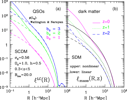
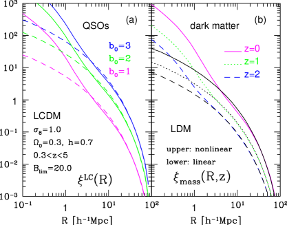
Fig. 1: Two-point correlation functions in the cluster normalized standard CDM model. (a) $\xi^{LC}(R)$ defined on the light-cone hypersurface for QSOs with $B_{lim}=20$. We assume three cases for the biasing parameter, $b_{0}=3$, 2 and 1, from top to bottom. A nonlinear mass correlation function[12]is used for the solid lines, while the linear theory is used for dashed lines. (b) Linear (lower curves) and nonlinear[12](upper curves) mass correlation functions defined on the constant-time hypersurfaces $z=0$, 1 and 2.

Fig. 2: Same as Fig. 2, but in a cluster normalized, low-density spatially flat CDM model.

The results are plotted in Figs. 2 and 2 for SCDM and LCDM models, respectively. The B-band limiting magnitude $B_{lim}=20$ roughly corresponds to the upcoming SDSS QSO sample. The corresponding evolution of the amplitude of the correlation at $R=15$$h^{-1}$Mpc is plotted in Fig. 3. In the specific bias model we adopted, the amplitude monotonically decreases with increasing $z$. This is inconsistent with an observational claim[16] that the QSO correlation amplitude increases as $z$. Given the theoretical uncertainties of the current theoretical understanding of the bias, it is premature to draw any decisive conclusion at this point. In fact, behavior consistent with the observational claim is obtained with a different model of bias.[5, 17] Nevertheless, this example illustrates the potential importance of the light-cone effect in understanding the evolution of the bias of high-redshift objects.

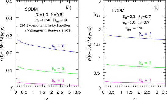
Fig. 3: Evolution of amplitudes of two-point correlation functions at $R=15{\hbox{$h^{-1}$}{\rm Mpc}}$ of QSOs on the light-cone in cluster normalized (a) standard and (b) low-density spatially flat CDM models.

2.3 Higher-order statistics on light-cone

Let us move to the higher-order statistics of clustering on the light-cone hypersurface. In particular we focus on the volume-averaged $N$-point correlation functions, $\overline{\xi}_{N}(R;z)$, at a redshift $z$ and on a comoving smoothing scale $R$. In the higher-order statistics, it is more useful to introduce the normalized higher-order moments $S_{N}(R;z)\equiv\overline{\xi}_{N}(R;z)/[\overline{\xi}_{2}(R;z)]^{N-1}$ than $\overline{\xi}_{N}(R;z)$. The hierarchical clustering ansatz states that $S_{N}(R;z)$ is constant and independent of the scale $R$. Moreover, $\overline{\xi}_{N}(R;z)$ evolves in proportion to $\left[\overline{\xi}_{2}(R;z)\right]^{N-1}$, and $S_{N}(R;z)$ is independent of $z$, according to perturbation theory.[18, 19]

As described in §2.1 and §2.2, however, the $N$-point correlation functions averaged over the light-cone,

$$\overline{\xi}_{N}(R;<z_{\rm max})\equiv{\displaystyle\int_{0}^{z_{\rm max}}z^{2}dz~{}w(z)\overline{\xi}_{N}(R;z)\,\over\displaystyle\int_{0}^{z_{\rm max}}z^{2}dz~{}w(z)},$$ (2.23)

and the corresponding moments,

$$\overline{S_{N}}(R;<z_{\rm max})\equiv{\overline{\xi}_{N}(R;<z_{\rm max})\over\left[\overline{\xi}_{2}(R;<z_{\rm max})\right]^{N-1}},$$ (2.24)

are the statistics more directly estimated from redshift surveys than their counterparts defined on the idealistic $z=0$ hypersurface. Note that the expression (2.23) looks slightly different from Eq. (2.12). This is because we have count-in-cell analysis in mind with the sampling cells being placed randomly in the $z$-coordinate. The effect of the selection function is taken into account by the weight function $w(z)$. In the case of count-in-cell analysis, one can correct for the selection function $\phi(z)$ by multiplying the count in cells located at $z$ by $1/\phi(z)$. Then $w(z)$ can be set to unity for $z<z_{\rm max}$ and zero for $z>z_{\rm max}$ in principle, where $z_{\rm max}$ is the maximum redshift of the sample. In the remainder of this subsection, we assume that the effect of the selection function is already corrected in this way, and consider the light-cone effect on the moments (2.24) due to the difference of the gravitational evolution within the survey volume.

Let us define a function $G$ which describes the evolution of the averaged two-point correlation function at $R$ and $z$:

$$\overline{\xi}(R;z)=G(R;z)\overline{\xi}(R;0).$$ (2.25)

In general, $G$ is not a simple function of $R$ and $z$, but a complicated functional of $\xi$. In the linear regime, however, $G$ is independent of $R$ and given by $[D(z)/D(0)]^{2}$, and even in the nonlinear regime, it is known that $G$ is approximately expressed as a function of $R$ and $z$ alone. To proceed more specifically, we apply the fitting formula[20] which relates the evolved two-point correlation function $\overline{\xi}_{E}(R;z)$ with its linear counterpart $\overline{\xi}_{L}(R_{0};z)$ as follows:

$$\halign to=0.0pt{\@eqnsel\hskip\@centering$\displaystyle{#}$&\global\@eqcnt\@ne\hskip 2\arraycolsep\hfil${#}$\hfil&\global\@eqcnt\tw@\hskip 2\arraycolsep$\displaystyle{#}$\hfil&\llap{#}\cr 0.0pt plus 1000.0pt$\displaystyle{{} \overline{\xi}_{E}(R;z) &12.0pt\hfil${=&12.0pt$\displaystyle{B(n) \, F[\overline{\xi}_{L}(R_{0};z)/B(n)] ,{}&\hbox to0.0pt{\hss{\rm(2\raise 2.15277pt\hbox{.}26a)\hskip 10.00002pt}\cr\penalty 100\vskip 3.0pt\vskip 0.0pt\cr 0.0pt plus 1000.0pt$\displaystyle{{} F(x) &12.0pt\hfil${=&12.0pt$\displaystyle{{x+0.45 x^{2} -0.02 x^{5}+0.05 x^{6} \over 1+0.02 x^{3} + 0.003 x^{9/2}} . &\hbox to0.0pt{\hss{\rm(2\raise 2.15277pt\hbox{.}26b)\hskip 10.00002pt}\cr}}}}}}}}}$$

In the above equations, $n$ denotes the effective spectral index of the power spectrum evaluated at the scale just entering the nonlinear regime, $R_{0}=[1+\overline{\xi}_{E}(z,R)]^{1/3}R$, and $B(n)=[(3+n)/3]^{0.8}$.

The inverse of Eq. (LABEL:eq:jmwfit1) is also empirically fitted as follows:

$$\halign to=0.0pt{\@eqnsel\hskip\@centering$\displaystyle{#}$&\global\@eqcnt\@ne\hskip 2\arraycolsep\hfil${#}$\hfil&\global\@eqcnt\tw@\hskip 2\arraycolsep$\displaystyle{#}$\hfil&\llap{#}\cr 0.0pt plus 1000.0pt$\displaystyle{\overline{\xi}_{L}(R_{0};z) &12.0pt\hfil${=&12.0pt$\displaystyle{B(n) F^{-1}[\overline{\xi}_{E}(R;z)/B(n)] ,{}&\hbox to0.0pt{\hss{\rm(2\raise 2.15277pt\hbox{.}27a)\hskip 10.00002pt}\cr\penalty 100\vskip 3.0pt\vskip 0.0pt\cr 0.0pt plus 1000.0pt$\displaystyle{F^{-1}(y) &12.0pt\hfil${=&12.0pt$\displaystyle{y\left( {1+ 0.036 y^{1.93} +0.0001 y^{3} \over 1+1.75 y -0.0015 y^{3.63} +0.028 y^{4}} \right)^{1/3} . {} &\hbox to0.0pt{\hss{\rm(2\raise 2.15277pt\hbox{.}27b)\hskip 10.00002pt}\cr}}}}}}}}}$$

Then the scale-dependent evolution factor $G(z)=G(R;z)$ defined by Eq. (2.25) is expressed explicitly in terms of $\overline{\xi}_{E}(R;0)$:

$$G(R;z)\equiv{\overline{\xi}_{E}(R;z)\over\overline{\xi}_{E}(R;0)}=\frac{B(n)}{\overline{\xi}_{E}(R;0)}F\left[{D^{2}(z)\over D^{2}(0)}F^{-1}\left({\overline{\xi}_{E}(R,0)\over B(n)}\right)\right].$$ (2.28)

Substituting the evolution law (2.25), Eq. (2.24) is explicitly written as

$$\overline{S_{N}}(R;<z_{\rm max}) = \left[\int_{0}^{z_{\rm max}}z^{2}dz~{}w(z)\right]^{N-2}{\hbox{$\left/\vbox to0.0pt{}\right.\n@space$}}\left[\int_{0}^{z_{\rm max}}z^{2}dz~{}w(z)G(R;z)\right]^{N-1}$$ (2.29)

$$\times \int_{0}^{z_{\rm max}}z^{2}dz~{}w(z)S_{N}(R;z)\left\{G(R;z)\right\}^{N-1}$$

In order to proceed further, we assume that $S_{N}(R;z)$ does not evolve with $z$, i.e., $S_{N}(R;z)=S_{N}(R;0)$. As described above, this is a reasonable approximation as long as objects are unbiased tracers of the underlying density field. Also let us introduce the measure of the light-cone effect:

$$\mathchar 28929\relax_{N}(R;<z_{\rm max})\equiv{\overline{S_{N}}(R;<z_{\rm max})\over S_{N}(R;0)}-1.$$ (2.30)

Then $(1+\mathchar 28929\relax_{N})$ can be regarded as a correction factor for the $S_{N}$ estimated without considering the light-cone effect. This quantifies the importance of the light cone effect on the higher-order clustering statistics in future surveys. Using Eqs. (2.29) and (2.28) and assuming $S_{N}(z)=S_{N}(0)$, we evaluate $\mathchar 28929\relax_{N}(<z_{\rm max})$ for SCDM, LCDM, and OCDM, which have $(\mathchar 28938\relax_{0},\lambda_{0},h,\sigma_{8})$ $=(1.0,0.0,0.5,0.56)$, $(0.3,0.7,0.7,1.0)$, and $(0.3,0.7,0.0,1.0)$, respectively. Figure 5 displays $\mathchar 28929\relax_{N}(R;<z)$ as a function of $z$, while Figure 5 plots $\mathchar 28929\relax_{N}(R;<z)$ against $R$.

Fig. 4: $\log_{10}\mathchar 28929\relax_{N}(R;z)$ are shown as functions of $\log_{10}z$ at $R=1{\hbox{$h^{-1}$}{\rm Mpc}}$ (left panels) and $10{\hbox{$h^{-1}$}{\rm Mpc}}$ (right panels). The curves correspond to $N=3,\ldots,N=10$ from bottom to top with $N=3$ and $N=7$ plotted in thick lines (from Ref. ?).

Fig. 5: $\log_{10}\mathchar 28929\relax_{N}(R;z)$ are displayed as functions of $\log_{10}R$ at $z=0.2$ (left panels) and $1.0$ (right panels). The curves correspond to $N=3,\ldots,N=10$ from bottom to top with $N=3$ and $N=7$ plotted in thick lines (from Ref. ?).

The figures suggest that the light-cone effect is quite robust.Although its details depend on the model, the difference is fairly small, and qualitatively all models behave similarly; the magnitude of the correction monotonically increases for higher order $N$. Also as expected, the light-cone effect becomes larger as $z_{\rm max}$ increases (Fig. 5). Although the correction is relatively small for shallow surveys with $z\lower 2.15277pt\hbox{$\;\buildrel<\over{\sim}\;$}0.2$ samples, $\mathchar 28929\relax_{N}(R;<z_{\rm max})$ becomes $\lower 2.15277pt\hbox{$\;\buildrel>\over{\sim}\;$}10$% in nonlinear scales ($R\sim 1{\hbox{$h^{-1}$}{\rm Mpc}}$). In SCDM, for instance, $\mathchar 28929\relax_{N}(R;<z_{\rm max})$ exceeds unity for $N\geq 6$ for the entire dynamic range plotted. Furthermore, Fig. 5 indicates that even if the hierarchical ansatz is correct (i.e., $S_{N}(R;z)$ is independent of $R$), the light-cone effect should generate apparent scale-dependence, since the correction behaves differently at different scales for a given redshift. In future surveys extending to $z>1$, Fig.  5 implies that the required correction for the light-cone effect is appreciable, ranging from up to unity for $S_{3}$ through factors of few for $S_{6}$ to factors of hundred for $S_{10}$.

3 Cosmological redshift-space distortion

3.1 Basic idea of cosmological redshift-space distortion

The approach described in §2 is based on an implicit idea to treat all objects in a survey catalogue simultaneously. If the number of objects in the catalogue is sufficiently large, one can divide the objects in many redshift bins. Then the light-cone effect discussed above is less important, as long as one treats each individual bin separately. In this case, however, another interesting effect due to the geometry of the universe emerges. This originates from the fact that the (observable) redshift-space separation $\bf s$ is mapped to the (unobservable) comoving separation $\bf x$ of objects at $z$ differently, depending on whether the separation is parallel or perpendicular to the line-of-sight direction of an observer at $z=0$. Due to this effect, a sphere located at $z$ becomes elongated along the line-of-sight in general.[21] In this section, we describe the anisotropy in the two-point correlation function of high-redshift objects induced by this effect, which we call the cosmological redshift-space distortion,[7, 22] in order to distinguish the conventional redshift-space distortion due to the peculiar velocity field.[23]${}^{\hbox{\,-}}$[26]

Fig. 6: Behavior of $c_{\scriptscriptstyle\parallel}(z)$ and $c_{\scriptscriptstyle\perp}(z)$ for ($\mathchar 28938\relax_{0}$, $\lambda_{0}$) = (0.3,0.7), (1.0,0.0), and (0.3,0.0) corresponding to the solid, dashed and dotted lines, respectively.

Throughout this section, we assume a standard Robertson – Walker metric of the form

$$ds^{2}=-dt^{2}+a(t)^{2}\{d\chi^{2}+S(\chi)^{2}[d\theta^{2}+\sin^{2}\theta d\phi^{2}]\}.$$ (3.1)

We adopt a normalization for which the present scale factor $a_{0}$ is unity. Then the spatial curvature $K$ is related to the other parameters as

$$K=H_{0}^{2}(\mathchar 28938\relax_{0}+\lambda_{0}-1),$$ (3.2)

and $S(\chi)$ is determined by the sign of $K$ according to

$$S(\chi)=\left\{\begin{array}[]{ll}\sin{(\sqrt{K}\chi)}/\sqrt{K}&\mbox{$(K>0)$}\\ \chi&\mbox{$(K=0)$}\\ \sinh{(\sqrt{-K}\chi)}/\sqrt{-K}&\mbox{$(K<0)$}\end{array}\right..\\$$

The radial distance $\chi(z)$ is given by

$$\chi(z)=\int_{t}^{t_{0}}{dt\over a(t)}=\int_{0}^{z}{dz\over H(z)}.$$ (3.3)

Fig. 7: Effect of inhomogeneity on the angular diameter distance $D_{\scriptscriptstyle A}(z)$ (upper panels) and the correction factor $\eta(z)=c_{\scriptscriptstyle\parallel}(z)/c_{\scriptscriptstyle\perp}(z)$ (lower panels) for $\lambda_{0}=0$ and $0.9$ models in $\mathchar 28938\relax_{0}=1$ (left panels) and $\mathchar 28938\relax_{0}=0.1$ (right panels) universes. Thick lines indicate the results for the empty beam ($\alpha=0)$, while thin lines for the filled beam ($\alpha=1)$.

Consider a pair of objects located at redshifts $z_{1}$ and $z_{2}$. If both the redshift difference $\delta z\equiv z_{1}-z_{2}$ and the angular separation of the pair $\delta\theta$ are much less than unity, the comoving separations of the pair parallel and perpendicular to the line-of-sight direction, $x_{{\scriptscriptstyle\parallel}}$ and $x_{\scriptscriptstyle\perp}$, are given by

$$x_{{\scriptscriptstyle\parallel}}(z)={d\chi(z)\over dz}\delta z=\frac{c_{{\scriptscriptstyle\parallel}}\delta z}{H_{0}},\quad x_{\scriptscriptstyle\perp}(z)=S(\chi(z))\delta\theta=\frac{c_{\scriptscriptstyle\perp}z\delta\theta}{H_{0}},$$ (3.4)

where $c_{\scriptscriptstyle\parallel}(z)=H_{0}/H(z)$, $c_{\scriptscriptstyle\perp}(z)=H_{0}S(\chi(z))/z$ and $z\equiv(z_{1}+z_{2})/2$. Thus their ratio becomes

$${x_{\scriptscriptstyle\parallel}(z)\over x_{\scriptscriptstyle\perp}(z)}=\frac{c_{\scriptscriptstyle\parallel}(z)}{c_{\scriptscriptstyle\perp}(z)}{\delta z\over z\delta\theta}\equiv\eta(z){\delta z\over z\delta\theta}.$$ (3.5)

Since $\delta z/(z\delta\theta)$ is the ratio of the parallel and perpendicular separations to the line-of-sight direction, $\eta(z)$ represents the distortion in the redshift space coordinates induced by the geometry of the universe. Typical behavior of $c_{\scriptscriptstyle\parallel}(z)$, $c_{\scriptscriptstyle\perp}(z)$ and $\eta(z)$ is plotted in Fig. 6 and the lower panels of Fig. 7. This is purely a general relativistic effect which was first proposed as a potential test of the cosmological constant.[21]

Actually it took a couple of decades to find realistic phenomena to which the test could be applied observationally. Recently two independent groups[7, 22] proposed to use the anisotropy in the clustering pattern of quasars and galaxies at high-redshifts as a probe of $\eta(z)$. The next subsections describe the methodology in linear theory, and then examine the feasibility in the nonlinear regime using $N$-body simulations.[27]

3.2 Linear theory of cosmological redshift-space distortion

We choose a fiducial point at redshift $z$ as an origin, and set up locally Euclidean coordinates with respect to this point. Let us adopt the distant (plane-parallel) observer approximation and choose the line-of-sight direction as the third axis. Then, if an object is located at ${\bf x}=(x_{1},x_{2},x_{3})$ in the real (comoving) space, the corresponding redshift-space coordinates, ${\mbox{\boldmath$s$}}=(s_{1},s_{2},s_{3})$, observed at $z=0$ are written as

$$\halign to=0.0pt{\@eqnsel\hskip\@centering$\displaystyle{#}$&\global\@eqcnt\@ne\hskip 2\arraycolsep\hfil${#}$\hfil&\global\@eqcnt\tw@\hskip 2\arraycolsep$\displaystyle{#}$\hfil&\llap{#}\cr 0.0pt plus 1000.0pt$\displaystyle{s_{1} &12.0pt\hfil${=&12.0pt$\displaystyle{\frac{x_{1}}{c_{\scriptscriptstyle\perp}(z)}, {}&\hbox to0.0pt{\hss{\rm(3\raise 2.15277pt\hbox{.}6a)\hskip 10.00002pt}\cr\penalty 100\vskip 3.0pt\vskip 0.0pt\cr 0.0pt plus 1000.0pt$\displaystyle{s_{2} &12.0pt\hfil${=&12.0pt$\displaystyle{\frac{x_{2}}{c_{\scriptscriptstyle\perp}(z)}, {}&\hbox to0.0pt{\hss{\rm(3\raise 2.15277pt\hbox{.}6b)\hskip 10.00002pt}\cr\penalty 100\vskip 3.0pt\vskip 0.0pt\cr 0.0pt plus 1000.0pt$\displaystyle{s_{3} &12.0pt\hfil${=&12.0pt$\displaystyle{\frac{z_{\rm obs} - z}{H_{0}} \simeq{1 \over c_{\scriptscriptstyle\parallel}(z)} \left[x_{3} + \frac{1 + z}{H(z)}v_{{\scriptscriptstyle\parallel}} \right] . &\hbox to0.0pt{\hss{\rm(3\raise 2.15277pt\hbox{.}6c)\hskip 10.00002pt}\cr}}}}}}}}}}}}}$$

In the last expression, $v_{{\scriptscriptstyle\parallel}}$ is the recession velocity of the object relative to the observer, and $z\ll H(z)x_{3}$ is assumed. Computing the Jacobian of the above transformation in linear theory, one can relate the density contrasts of the objects in real and redshift spaces as

$$\delta^{(s)}({\mbox{\boldmath$s$}}({\bf x}))=\delta^{(r)}({\bf x})-\frac{1+z}{H(z)}\partial_{3}v_{\scriptscriptstyle\parallel}.$$ (3.7)

The peculiar velocity in linear theory is written in terms of the mass density contrast $\delta_{\rm\scriptscriptstyle mass}$ as[28]

$$v_{\scriptscriptstyle\parallel}({\bf x})=-\frac{H(z)}{1+z}f(z)\partial_{3}\triangle^{-1}\delta_{\rm\scriptscriptstyle mass}({\bf x}),$$ (3.8)

where $\triangle^{-1}$ is the inverse Laplacian, and

$$\halign to=0.0pt{\@eqnsel\hskip\@centering$\displaystyle{#}$&\global\@eqcnt\@ne\hskip 2\arraycolsep\hfil${#}$\hfil&\global\@eqcnt\tw@\hskip 2\arraycolsep$\displaystyle{#}$\hfil&\llap{#}\cr 0.0pt plus 1000.0pt$\displaystyle{ f(z) &12.0pt\hfil${\equiv&12.0pt$\displaystyle{\frac{d\ln D(z)}{d\ln a} \simeq\mathchar 28938\relax(z)^{0.6} + {\lambda(z) \over 70} \left(1+ {\mathchar 28938\relax(z) \over 2}\right), {}&\hbox to0.0pt{\hss{\rm(3\raise 2.15277pt\hbox{.}9a)\hskip 10.00002pt}\cr\penalty 100\vskip 3.0pt\vskip 0.0pt\cr 0.0pt plus 1000.0pt$\displaystyle{\mathchar 28938\relax(z) &12.0pt\hfil${=&12.0pt$\displaystyle{\left[{H_{0} \over H(z)}\right]^{2} \, (1+z)^{3} \mathchar 28938\relax_{0} ,{}&\hbox to0.0pt{\hss{\rm(3\raise 2.15277pt\hbox{.}9b)\hskip 10.00002pt}\cr\penalty 100\vskip 3.0pt\vskip 0.0pt\cr 0.0pt plus 1000.0pt$\displaystyle{\lambda(z) &12.0pt\hfil${=&12.0pt$\displaystyle{\left[{H_{0} \over H(z)}\right]^{2} \, \lambda_{0} . &\hbox to0.0pt{\hss{\rm(3\raise 2.15277pt\hbox{.}9c)\hskip 10.00002pt}\cr}}}}}}}}}}}}}$$

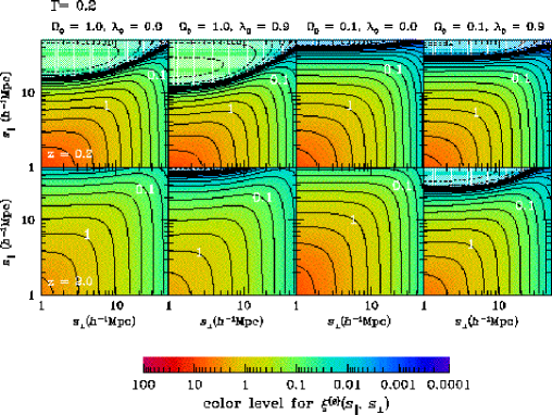
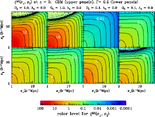
Fig. 8: Contours of $\xi^{(s)}(s_{\scriptscriptstyle\perp},s_{{\scriptscriptstyle\parallel}})$ for the fixed shape parameter $\mathchar 28928\relax$ ($=0.2$) and $\sigma_{8}=1.0$ models at $z=0.2$ (upper panels) and $z=2.0$ (lower panels); $(\mathchar 28938\relax_{0},\lambda_{0})=(1.0,0.0)$, $(1.0,0.9)$, $(0.1,0.0)$ and $(0.1,0.9)$ from left to right. Solid and dashed lines indicate the positive and negative $\xi^{(s)}$, respectively. Contour spacings are $\mathchar 28929\relax{\rm log}_{10}|\xi|=0.25$.

Fig. 9: Contours of $\xi^{(s)}(s_{\scriptscriptstyle\perp},s_{{\scriptscriptstyle\parallel}})$ at $z=3$. Upper and lower panels correspond to the COBE-normalized CDM models (the shape parameter $\mathchar 28928\relax$ is given by Eq. (LABEL:eq:gamma)), the fixed $\mathchar 28928\relax$ ($=0.2$) models with $\sigma_{8}=1.0$. Contour spacings and line types are the same as in Fig. 9.

In order to close the equations, one has to relate the density contrast of objects in real space $\delta^{(r)}$ to that of mass, $\delta_{\rm\scriptscriptstyle mass}$, by specifying the model of bias. As in §2.2, we adopt a linear bias:

$$\delta^{(r)}({\bf x};z)=b(z)\delta_{\rm\scriptscriptstyle mass}({\bf x};z).$$ (3.10)

Substituting the above equations into Eq. (3.7), we obtain

$$\delta^{(s)}({\mbox{\boldmath$s$}}({\bf x}))=\int\frac{d^{3}k}{(2\pi)^{3}}\left[1+\beta(z)\frac{k_{3}^{\;2}}{k^{2}}\right]e^{i{\bf k}\cdot{\bf x}}{\widetilde{\delta}}^{(r)}({\bf k}),$$ (3.11)

where $\beta(z)=f(z)/b(z)$, and ${\widetilde{\delta}}^{(r)}$ is the Fourier transform of $\delta^{(r)}$. Repeating the method of Hamilton (1992),[25] we obtain an explicit formula for the redshift-space two-point correlation function which is valid at arbitrary $z$ in linear theory:

$$\halign to=0.0pt{\@eqnsel\hskip\@centering$\displaystyle{#}$&\global\@eqcnt\@ne\hskip 2\arraycolsep\hfil${#}$\hfil&\global\@eqcnt\tw@\hskip 2\arraycolsep$\displaystyle{#}$\hfil&\llap{#}\cr 0.0pt plus 1000.0pt$\displaystyle{ \xi^{(s)}(s_{\scriptscriptstyle\perp}, s_{\scriptscriptstyle\parallel}) &12.0pt\hfil${=&12.0pt$\displaystyle{\left(1+{2\over 3}\beta(z) +{1\over 5}[\beta(z)]^{2}\right) \xi_{0}(x) P_{0}(\mu) \cr 0.0pt plus 1000.0pt$\displaystyle{&12.0pt\hfil${-&12.0pt$\displaystyle{\left({4\over 3}\beta(z) +{4\over 7}[\beta(z)]^{2}\right)\xi_{2}(x) P_{2}(\mu) \cr 0.0pt plus 1000.0pt$\displaystyle{&12.0pt\hfil${+&12.0pt$\displaystyle{\frac{8}{35}[\beta(z)]^{2} \xi_{4}(x) P_{4}(\mu) , {}&\hbox to0.0pt{\hss{\rm(3\raise 2.15277pt\hbox{.}12a)\hskip 10.00002pt}\cr\penalty 100\vskip 3.0pt\vskip 0.0pt\cr 0.0pt plus 1000.0pt$\displaystyle{\xi_{2l}(x) &12.0pt\hfil${=&12.0pt$\displaystyle{{1 \over 2\pi^{2}} \int_{0}^{\infty}dk k^{2} j_{2l}(kx) P(k;z) , {}&\hbox to0.0pt{\hss{\rm(3\raise 2.15277pt\hbox{.}12b)\hskip 10.00002pt}\cr\penalty 100\vskip 3.0pt\vskip 0.0pt\cr 0.0pt plus 1000.0pt$\displaystyle{P(k;z) &12.0pt\hfil${=&12.0pt$\displaystyle{[b(z)]^{2}\left[\frac{D(z)}{D(0)}\right]^{2} P^{\rm\scriptscriptstyle mass}(k;z=0). &\hbox to0.0pt{\hss{\rm(3\raise 2.15277pt\hbox{.}12c)\hskip 10.00002pt}\cr}}}}}}}}}}}}}}}}}}}$$

In the above, $x\equiv\sqrt{{c_{\scriptscriptstyle\parallel}}^{2}{s_{\scriptscriptstyle\parallel}}^{2}+{c_{\scriptscriptstyle\perp}}^{2}{s_{\scriptscriptstyle\perp}}^{2}}$, $\mu\equiv c_{{\scriptscriptstyle\parallel}}s_{{\scriptscriptstyle\parallel}}/x$ ($s_{\scriptscriptstyle\parallel}=s_{3}$ and $s_{\scriptscriptstyle\perp}^{2}=s_{1}^{2}+s_{2}^{2}$), the $P_{n}$ are the Legendre polynomials, i.e., $P_{0}(\mu)=1$, $P_{2}(\mu)=(3\mu^{2}-1)/2$, and $P_{4}(\mu)=(35\mu^{4}-30\mu^{2}+3)/8$. Figure 9 plots $\xi^{(s)}(s_{\scriptscriptstyle\perp},s_{{\scriptscriptstyle\parallel}})$ for $\mathchar 28928\relax=0.2$ and $\sigma_{8}=1.0$ models to illustrate the degree of distortion. Figure 9 shows the difference between CDM models with $\mathchar 28928\relax$ of Eq. (LABEL:eq:gamma) and fixed $\mathchar 28928\relax(=0.2)$ models with the same $\mathchar 28938\relax_{0}$ and $\lambda_{0}$.

3.3 Implication for galaxy redshift surveys

The cosmological distortion effect becomes important also even for shallower galaxy redshift surveys.[29] One may formally expand $\xi^{(s)}(s_{\scriptscriptstyle\perp},s_{{\scriptscriptstyle\parallel}})$ in terms of the observables, $s\equiv\sqrt{s_{{\scriptscriptstyle\parallel}}^{2}+s_{\scriptscriptstyle\perp}^{2}}$ and $\mu_{s}\equiv s_{{\scriptscriptstyle\parallel}}/s$, instead of the unobservable variables ($x(z)$, $\mu_{x}(z)$):

$$\xi^{(s)}(s_{\scriptscriptstyle\perp},s_{{\scriptscriptstyle\parallel}};z)=\sum_{l=0}^{2}\xi_{2l}(x;z)P_{2l}(\mu_{x})=\sum_{l=0}^{\infty}\zeta^{(s)}_{2l}(s;z)P_{2l}(\mu_{s}).$$ (3.13)

Since we are interested in surveys for which $z\ll 1$, we can further expand the above summation up to first order in $z$, and then obtain

$$\xi^{(s)}(s_{\scriptscriptstyle\perp},s_{{\scriptscriptstyle\parallel}};z)\approx\sum_{l=0}^{3}\zeta^{(s)}_{2l}(s;z)P_{2l}(\mu_{s}).$$ (3.14)

The explicit expressions for $\zeta^{(s)}_{2l}(s;z)$ of the form:

$$\zeta^{(s)}_{2l}(x;z)=\xi^{(s)}_{0}(x;0)+\delta_{2l}z$$ (3.15)

for $l=0$, 1, 2 and 3 are found in Ref. ?.

One possible application of those perturbative formulae is to estimate a systematic error for the $\beta$-parameter, $\beta_{0}$, due to the neglect of the cosmological redshift-space distortion. Hamilton (1992) proposed to estimate $\beta_{0}$ from the moments of the observed two-point correlation functions of galaxies on the basis of the relation[25]

$$\frac{1+2\beta_{0}/3+\beta_{0}^{2}/5}{4\beta_{0}/3+4\beta_{0}^{2}/7}=\frac{\xi^{(s)}_{0}(r;0)}{\xi^{(s)}_{2}(r;0)}-3\int_{0}^{r}\frac{\xi^{(s)}_{0}(x;0)}{\xi^{(s)}_{2}(r;0)}\left({x\over r}\right)^{3}{dx\over x}.$$ (3.16)

If one takes account of the cosmological redshift-space distortion at $z$, $\xi^{(s)}_{0}(x;0)$ and $\xi^{(s)}_{2}(x;0)$ on the right-hand side of the above equation should be replaced by $\zeta^{(s)}_{0}(x;z)$ and $\zeta^{(s)}_{2}(x;z)$, respectively. Then substituting the perturbation expansion (3.15) into Eq. (3.16), one can compute the systematic error for $\beta_{0}$ defined through

$$\beta(z)=\beta_{0}+\epsilon z.$$ (3.17)

The result[8] consists of the two terms corresponding to the evolution of the $\beta$-parameter and the geometrical effect:

$$\epsilon=\left.{d\,\beta(z)\over dz}\right|_{z=0}+{1+q_{0}\over 1+6\beta_{0}/7+3\beta_{0}^{2}/35}\times\left[{\beta_{0}\over 7}\left(1-{\beta_{0}\over 5}-{11\beta_{0}^{2}\over 15}-{\beta_{0}^{3}\over 7}\right)\right.$$

$$\hskip 56.9055pt\left.+\frac{1/4+3\beta_{0}/7+17\beta_{0}^{2}/70+\beta_{0}^{3}/21+\beta_{0}^{4}/196}{{3\over r^{3}}\int_{0}^{r}[\xi(x;0)-\xi(r;0)]x^{2}dx}\,{\partial\xi(r;0)\over\partial\ln r}\right],$$ (3.18)

where $q_{0}$ is the deceleration parameter ($=\mathchar 28938\relax_{0}/2-\lambda_{0}$). For magnitude-limited samples, the above expression should be averaged over the sample with an appropriate weight according to the selection function. If the magnitude limit of the survey is 18.5 (in B-band) as in the SDSS galaxy redshift sample, the systematic error ranges between $-20\%$ and $10\%$, depending on the cosmological parameters. Although such systematic errors are smaller than the statistical errors in the current surveys, they will definitely dominate the expected statistical error for future surveys.

3.4 Effects of the cosmological distance and evolution of bias

Here we discuss two potentially important effects, which were ignored in §3.1 to §3.3, on the cosmological redshift-space distortion: the effect of inhomogeneities in the light propagation and the evolution of bias.

The angular diameter distance $D_{\scriptscriptstyle A}$, which plays a key role in the geometrical test at high $z$, depends sensitively on the inhomogeneous matter distribution as well as $\lambda_{0}$ and the density parameter $\mathchar 28938\relax_{0}$. A reasonably realistic approximation to the light propagation in an inhomogeneous universe is given by the Dyer – Roeder distance.[30] It assumes that the fraction $\alpha$ of the total matter in the universe is distributed smoothly and the rest is in clumps. If an observed beam of light propagates far from any clump, then the angular diameter distance $D_{\scriptscriptstyle A}(z;\alpha,\mathchar 28938\relax_{0},\lambda_{0})$ satisfies

$${d^{2}D_{\scriptscriptstyle A}\over dz^{2}}+\left[{2\over 1+z}+{1\over H(z)}{dH(z)\over dz}\right]{dD_{\scriptscriptstyle A}\over dz}+{3\over 2}{\alpha H_{0}^{2}\mathchar 28938\relax_{0}(1+z)\over H(z)^{2}}D_{\scriptscriptstyle A}=0,$$ (3.19)

with $D_{\scriptscriptstyle A}(z=0)=0$ and $dD_{\scriptscriptstyle A}/dz(z=0)=1/H_{0}$. The preceding discussion on the cosmological redshift-space distortion adopted a standard distance, which corresponds to the extreme case of $\alpha=1$. As shown in Fig. 7, the effect of inhomogeneity represented by the parameter $\alpha$ in the above approximation, however, could be large for high $z$ if $\alpha$ is significantly different from unity. Another uncertainty will come from the possible time-dependence of the bias parameter $b(z)$. As we emphasized in the discussion of the light-cone effect, we do not yet have any reliable theoretical model for bias. Thus we adopt the linear bias model (2.17) so as to highlight the effect of the evolution of bias in the present context.

Fig. 10: Evolution of bias and $\beta(z)$. Dashed and solid lines correspond to constant biasing parameter $b(z)=2$ and $1$, respectively, while dotted lines correspond to the bias model (Eq. (2.17)) with $b=2$ at $z=0$. Thick and thin lines correspond to $\lambda_{0}=0.9$ and $0$, respectively.

Figure 7 may seem to indicate that inhomogeneity makes even a larger difference than that of $\lambda_{0}$, especially for $z\gg 1$. In reality, however, the situation is not so bad; since the expectation value of $\alpha$ is determined by the effective volume of the beam of the light bundles, it depends on the depth $z$ and the angular separation $\delta\theta$ (of the quasar pair in the present example). For larger $z$ and larger $\delta\theta$, $\alpha(z,\delta\theta)$ should approach unity in any case, and the result based on the standard distance as in §3.1 to §3.3 would be more appropriate and closer to the truth. Since we do not have any justifiable model for $\alpha(z,\delta\theta)$, we will consider two extreme cases, $\alpha(z,\delta\theta)=1$ (filled beam) and $0$ (empty beam). Our main purpose here is to highlight the importance of the effect, even though more realistically $\alpha(z,\delta\theta)$ is somewhere between the two extreme cases; it is shown that $\alpha(z,\delta\theta)=1$ is a good approximation for $z\gg 1$ and $\delta\theta\gg 1$.[31]

It is quite reassuring that even in these extreme cases the inhomogeneity effect is much weaker than that of $\lambda_{0}$ up to $z\lower 2.15277pt\hbox{$\;\buildrel<\over{\sim}\;$}2$ in low density universes, as the right panels in Fig. 7 illustrate clearly. Since a relatively low value of $\mathchar 28938\relax_{0}$ around $0.1-0.3$ is favored observationally,[28] the optimal redshift to determine $\lambda_{0}$ in low $\mathchar 28938\relax_{0}$ universes is $z=1-2$.

Fig. 11: The anisotropy parameter $\xi^{(s)}_{{\scriptscriptstyle\parallel}}(s)/\xi^{(s)}_{\scriptscriptstyle\perp}(s)$ as a function of $z$ at $s=10h^{-1}$Mpc in cold dark matter universes with $H_{0}=70$km/sec/Mpc. The upper panels correspond to $\alpha=0$ (empty beams), while the lower panels correspond to $\alpha=1$ (filled beams).

Fig. 12: The anisotropy parameter $\xi^{(s)}_{{\scriptscriptstyle\parallel}}(s)/\xi^{(s)}_{\scriptscriptstyle\perp}(s)$ as a function of $s$ at $z=1$ (upper panels) and at $z=3$ (lower panels) in cold dark matter universes with $H_{0}=70$km/sec/Mpc. The left panels correspond to $\alpha=0$ (empty beams), while the right panels correspond to $\alpha=1$ (filled beams).

Figure 10 illustrated the evolution of bias (Eq. (2.17); upper panels) and of the resulting $\beta(z)$ parameter (lower panels). This implies that as long as Fry’s model of $b(z)$ is adopted, one can distinguish the value of $\lambda_{0}$ independently of the evolution of bias only in low density ($\mathchar 28938\relax_{0}\ll 1$) models and at intermediate redshifts ($z\lower 2.15277pt\hbox{$\;\buildrel<\over{\sim}\;$}2$). Together with the indication from Fig. 7, $z=1-2$ would be an optimal regime to probe $\lambda_{0}$ at least in low-density universes. Figure 12 illustrates the extent to which this is feasible simply on the basis of the anisotropy parameter,

$${\xi^{(s)}_{{\scriptscriptstyle\parallel}}(s)\over\xi^{(s)}_{\scriptscriptstyle\perp}(s)}\equiv{\xi^{(s)}(s_{\scriptscriptstyle\parallel}=0,s;z)\over\xi^{(s)}(s,s_{\scriptscriptstyle\perp}=0;z)},$$ (3.20)

adopting the power spectrum of the CDM models; in $\mathchar 28938\relax_{0}=1$ models the value of $\alpha$ completely changes the $z$-dependence of the anisotropy parameter while $\mathchar 28938\relax_{0}=0.1$ models are fairly insensitive to it. In addition, $\xi^{(s)}_{{\scriptscriptstyle\parallel}}(s)/\xi^{(s)}_{\scriptscriptstyle\perp}(s)$ for $z\lower 2.15277pt\hbox{$\;\buildrel<\over{\sim}\;$}2$ in $\mathchar 28938\relax_{0}=0.1$ models is basically determined by the biasing parameter at $z=0$ and less affected by the evolution of $b(z)$. Figure 12 shows the scale-dependence of the anisotropy parameter in $\mathchar 28938\relax_{0}=0.1$ and $h=0.7$ CDM models. This clearly indicates that one can distinguish the different $\lambda_{0}$ and bias models by analyzing the anisotropy of the correlation function at $z=1$ almost independently of $\alpha$.

3.5 Testing the redshift-space distortion with N-body simulations

As illustrated in Figs. 7 to 9, the two-point correlation functions become elongated along the line-of-sight due to the cosmological redshift-space distortion in linear theory. In reality, the finger of god due to the non-linear peculiar velocity affects the distortion pattern in the same direction. Therefore the proper modeling of the nonlinear effects is essential to estimate the cosmological parameters from the observed distortion. Also, the available number of observed objects would limit the statistical significance of the analysis. In order to examine these realistic effects in applying the redshift-space distortion as a cosmological test, we use a series of high-resolution N-body simulations.[32, 33, 27] The simulations assume the three representative cosmological models summarized in Table I. Each model has three realizations with different random seeds in generating the initial condition, and employs $N_{P}=256^{3}$ dark matter particles in the simulation volume of ($300h^{-1}$Mpc)³ (comoving). Figure 14 displays the results of $\xi^{(s)}(s_{\scriptscriptstyle\perp},s_{{\scriptscriptstyle\parallel}})$ at $z=2.2$ for these models. The upper panels plot the predictions in linear theory, the middle panels are computed from randomly sampled $N=5\times 10^{5}$ particles, and the lower panels from the $N=2\times 10^{4}$ most massive halos (groups of particles) identified,[32, 33] so as to take into account the effects of the finite sampling and the biasing to some degree.

Table I: Simulation model parameters.

Model	$\mathchar 28938\relax_{0}$	$\lambda_{0}$	$\mathchar 28928\relax$	$\sigma_{8}$	N	realizations
SCDM	1.0	0.0	0.5	0.6	$256^{3}$	3
OCDM	0.3	0.0	0.25	1.0	$256^{3}$	3
LCDM	0.3	0.7	0.21	1.0	$256^{3}$	3

Figure 14 plots the reduced $\chi^{2}$ contours from $\xi^{(s)}(s_{\scriptscriptstyle\perp},s_{{\scriptscriptstyle\parallel}})$ of simulations. Since our theoretical predictions do not include nonlinear effects at this point, we exclude the regions with $s_{{\scriptscriptstyle\parallel}}/s_{\scriptscriptstyle\perp}>2$, which are likely to be seriously contaminated by nonlinear peculiar velocities. While Fig. 14 demonstrates that the current methodology works in principle, the expected S/N is fairly low. This is largely because we adjusted the sampling rate for the high-z QSOs. The situation would be improved, though, if we apply the present methodology to a statistical sample of Lyman-break galaxies, for instance, whose number density is larger and their strong clustering is already observed.[2]

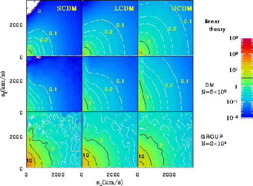
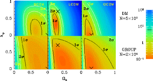
Fig. 13: $\xi^{(s)}(s_{\scriptscriptstyle\perp},s_{{\scriptscriptstyle\parallel}})$ at $z=2.2$ from linear theory (upper panels), and N-body simulations with $5\times 10^{5}$ randomly sampled particles (middle panels) and with $N=2\times 10^{4}$ most massive halos of particles (lower panels). The contour lines represent $\xi^{(s)}=10$, $10^{0.5}$ and $1$ (in black), and $\xi^{(s)}=0.5$, $0.3$, $0.2$ and $0.1$ (in white). The white region around the upper-left corner in SCDM model indicates $\xi^{(s)}<0$.

Fig. 14: The resulting $\chi^{2}$-contours in the $\mathchar 28938\relax_{0}$ - $\lambda_{0}$ plane from the analysis of the data in Fig. 14. The theoretical predictions are not corrected for the nonlinear effects. The crosses indicate the true values adopted in the simulation models.

In order to examine the nonlinear effects in the cosmological redshift-space distortion, we consider the power spectrum, rather than the two-point correlation functions, in which the phenomenological correction for the non-linear finger-of-god effect has already been discussed in the literature.[11, 22] Specifically, we model the power spectrum before the cosmological redshift-space distortion as

$$P^{(s)}(k,\mu)=P(k)[1+\beta\mu^{2}]^{2}D[k\mu\sigma_{P}],$$ (3.21)

where $\mu$ is the direction cosine in $k$ space, and the second factor on the right-hand-side comes from Eq. (3.11). The last factor is a phenomenological correction for non-linear velocity effect. We assume that the pair-wise velocity distribution in real space is exponential with a constant pairwise peculiar velocity along the line-of-sight, $\sigma_{P}$. In this case the damping term in Fourier space, $D[k\mu\sigma_{P}]$, is given by[11]

$$D[k\mu\sigma_{P}]=\frac{1}{1+(k\mu\sigma_{P})^{2}/2}.$$ (3.22)

Combining the geometrical effect, the power spectrum of objects at $z$ observed in redshift space is expressed as

$$P^{(CRD)}(k_{s{\scriptscriptstyle\perp}},k_{s{\scriptscriptstyle\parallel}};z) = \frac{1}{c_{\scriptscriptstyle\perp}(z)^{2}c_{\scriptscriptstyle\parallel}(z)}P^{(s)}(k_{\scriptscriptstyle\perp},k_{\scriptscriptstyle\parallel};z)$$ (3.23)

$$= \frac{1}{c_{\scriptscriptstyle\perp}(z)^{2}c_{\scriptscriptstyle\parallel}(z)}P(k;z)[1+\beta(z)\mu^{2}]^{2}D[k\mu\sigma_{P}(z)],\qquad$$ (3.24)

where the relation of the comoving wave numbers in real space, ${\bf k}$, and in cosmological redshift space, ${\bf k}_{s}$, is expressed as

$$k_{\scriptscriptstyle\perp}=\frac{k_{s{\scriptscriptstyle\perp}}}{c_{\scriptscriptstyle\perp}(z)},\qquad k_{\scriptscriptstyle\parallel}=\frac{k_{s{\scriptscriptstyle\parallel}}}{c_{\scriptscriptstyle\parallel}(z)},\qquad k=\sqrt{k_{\scriptscriptstyle\perp}^{2}+k_{\scriptscriptstyle\parallel}^{2}},\qquad\mu=\frac{k_{\scriptscriptstyle\parallel}}{k},$$ (3.25)

and $P(k;z)$ is a comoving real-space power spectrum at redshift $z$.

Clearly, the final expression for the redshift-space power spectrum $P^{(CRD)}(k_{s{\scriptscriptstyle\perp}},k_{s{\scriptscriptstyle\parallel}};z)$ depends on a number of parameters: $\mathchar 28938\relax_{0}$, $\lambda_{0}$, $\sigma_{8}$, $b(z)$, $P(k;z)$, and $\sigma_{P}(z)$. While none of these parameters has been determined precisely yet, there exist some tight constraints on them which can greatly reduce the number of the independent unknown parameters; provided that one adopts the linear biasing, the shape of the linear density power spectrum has already been determined fairly well by the APM galaxy survey, for instance.[35] The upcoming redshift surveys of nearby galaxies will improve this measurement significantly. Then, given $\sigma_{8}$ and $b(z)$, $P(k;z)$ is already accurately determined. Furthermore, with future large surveys which are pertinent to the analysis here, it should be fairly easy to determine $b(z)$ for a given cosmology. The pair-wise velocity dispersion $\sigma_{P}(R,z)$ at large separation can be determined by the other parameters through the cosmic energy equation:[34]

$$\halign to=0.0pt{\@eqnsel\hskip\@centering$\displaystyle{#}$&\global\@eqcnt\@ne\hskip 2\arraycolsep\hfil${#}$\hfil&\global\@eqcnt\tw@\hskip 2\arraycolsep$\displaystyle{#}$\hfil&\llap{#}\cr 0.0pt plus 1000.0pt$\displaystyle{ \sigma_{\rm p,MJB} &12.0pt\hfil${\equiv&12.0pt$\displaystyle{\langle v_{12}^{2}(r\rightarrow\infty)\rangle= \frac{2}{3}\langle v_{1}^{2}\rangle, {}&\hbox to0.0pt{\hss{\rm(3\raise 2.15277pt\hbox{.}26a)\hskip 10.00002pt}\cr\penalty 100\vskip 3.0pt\vskip 0.0pt\cr 0.0pt plus 1000.0pt$\displaystyle{\langle v_{1}^{2}\rangle&12.0pt\hfil${=&12.0pt$\displaystyle{\frac{3\mathchar 28938\relax(z)H^{2}(z)I_{2}(z)}{2(1+z)^{2}} \left[1-\frac{1+z}{D^{2}(z)}\int_{\frac{1}{1+z}}^{\infty}\frac{D^{2}(z')}{(1+z')^{2}}dz'\right] , {}&\hbox to0.0pt{\hss{\rm(3\raise 2.15277pt\hbox{.}26b)\hskip 10.00002pt}\cr\penalty 100\vskip 3.0pt\vskip 0.0pt\cr 0.0pt plus 1000.0pt$\displaystyle{I_{2}(z) &12.0pt\hfil${=&12.0pt$\displaystyle{\int_{0}^{\infty}\frac{dk}{k}\frac{\mathchar 28929\relax^{2}_{ }{\scriptscriptstyle{NL}} (k,z)}{k^{2}} &\hbox to0.0pt{\hss{\rm(3\raise 2.15277pt\hbox{.}26c)\hskip 10.00002pt}\cr}}}}}}}}}}}}}$$

Table II: Velocity dispersion $\sigma_{P}$ from theoretical predictions and the present simulations (in units of km/sec).

Model	$\sigma_{P,{\rm MJB}}(z=0)$	$\sigma_{P,{\rm sim}}(z=0)$	$\sigma_{P,{\rm MJB}}(z=2.2)$	$\sigma_{P,{\rm sim}}(z=2.2)$
SCDM	580	$591\pm 2$	164	$166\pm 1$
OCDM	599	$603\pm 6$	368	$364\pm 3$
LCDM	593	$606\pm 10$	380	$377\pm 4$

As Table II indicates, the above analytical fit is in good agreement with our simulation results. Finally, a constraint on $\sigma_{8}$ and $\mathchar 28938\relax_{0}$ from cluster abundances at $z=0$ is fairly well-established. Thus combining these model predictions and observational constraints, we will be left with only two unknown parameters, $\mathchar 28938\relax_{0}$ and $\lambda_{0}$, which we desire to determine from the cosmological redshift distortion.

Fig. 15: $P^{(s)}(k_{s{\scriptscriptstyle\perp}},k_{s{\scriptscriptstyle\parallel}})$ at $z=0$. The upper and lower panels display the linear theory predictions and the results from N-body simulations using all particles ($N=256^{3}$). The middle panels present our nonlinear model predictions on the basis of the non-linear power spectrum (Eq. ((ii) mass correlation function)). For the values of the pair-wise peculiar velocity dispersion $\sigma_{P}$, the solid lines correspond to those from the simulation data, while the dotted lines correspond to the analytical fitting formula (3.5). Contour spacings are $\mathchar 28929\relax\log_{10}P=0.5$, and the contours corresponding to $10^{5}$, $10^{4}$, $10^{3}$, $10^{2}$ and $10^{1}$ are plotted by the thick lines.

Fig. 16: The same as Fig. 16, but at $z=2.2$.

Figures 16 and 16 display the contour plots for $P^{(CRD)}(k_{s{\scriptscriptstyle\perp}},k_{s{\scriptscriptstyle\parallel}})$ at $z=0$ and $z=2.2$, respectively. The upper, middle, and lower panels correspond to theoretical predictions in linear theory, nonlinear model predictions on the basis of equations ((ii) mass correlation function) and (3.23), and simulation results, respectively. Note that $P(k)$ in this section is related to $\mathchar 28929\relax^{2}(k)$ in §2.2 as[11]

$$\mathchar 28929\relax^{2}(k)=\frac{1}{(2\pi)^{3}}4\pi k^{3}P(k).$$ (3.27)

The middle panels plot two nonlinear models which adopt different $\sigma_{P}$ in Eq. (3.22). The solid curves correspond to the pair-wise velocity dispersions directly evaluated from the simulation data, while the dotted curves correspond to an analytical fitting formula[34] (Eq. (3.5)). The right-hand-side of the above equation depends on the scale $R$ through a spherical top-hat window function, $W(k;R)$, while Eq. (3.22) is derived on the assumption that $\sigma_{P}(z)$ is scale-independent. Note that we adopt the velocity dispersion in comoving coordinates. This implies that we have to multiply the proper velocity by the conversion factor $H_{0}(1+z)/H(z)$. We adopt the value at $R=40h^{-1}$Mpc, which is the median value of the fitting range of our analysis (see below).

Fig. 17: $P^{(CRD)}(k_{s{\scriptscriptstyle\perp}},k_{s{\scriptscriptstyle\parallel}})$ at $z=2.2$ from N-body simulations using randomly sampled particles of $5\times 10^{5}$ (lower), $5\times 10^{4}$ (middle), and $5\times 10^{3}$ (upper). The contour levels are the same as those in Fig. 16.

As in the case of the two-point correlation functions, the degree to which one can recover the power spectrum sensitively depends on the number of sampled particles. The lower panels in Figs. 16 and 16 use all the simulation particles. We repeated the same analysis with randomly sampled $N_{P}=5\times 10^{5}$, $5\times 10^{4}$ and $5\times 10^{3}$ particles, and the results are displayed in Fig. 17. The SDSS QSO surveys, for instance, expect to have O($10^{4}$) QSOs between $z=1.5$ and $2.5$. This figure implies that although the phenomenological nonlinear models reproduce the simulation results very well, the statistical noise due to the limited numbers of QSOs will dominate the cosmological signal as long as one attempts to directly compare the $P^{(CRD)}(k_{s{\scriptscriptstyle\perp}},k_{s{\scriptscriptstyle\parallel}})$.

Fig. 18: The monopole moment, $P_{0}^{(CRD)}(k_{s})$, of the power spectrum in redshift space at $z=2.2$. The symbols indicate the mean values of 24 subsamples which randomly select $5\times 10^{4}$ particles from the entire set of simulation particles in three different realizations. The error bars are computed from the $1\sigma$ dispersions among the subsamples for each model. Five theoretical predictions are plotted with different types of curves. These values of $\sigma_{P}$ as curves correspond to various quoted in the plot.

One can increase the signal-to-noise ratio by expanding the power spectrum in multipole moments as

$$P_{l}^{(CRD)}(k_{s};z)\equiv\frac{2l+1}{2}\int^{1}_{-1}d\mu P^{(CRD)}(k_{s},\mu;z)P_{l}(\mu),$$ (3.28)

where the $P_{l}$ are the Legendre polynomials. In order to illustrate the higher signal-to-noise ratio in this approach, we plot the monopole term, $P_{0}^{(CRD)}(k_{s};z=2.2)$, in Fig. 18 computed from $5\times 10^{4}$ randomly sampled particles. The quoted error bars are estimated from the $1\sigma$ dispersions of $P_{0}$ of 24 random subsamples in total (eight randomly sampled particle sets for three different realizations). The five curves of different line types correspond to theoretical predictions which use different values for $\sigma_{P}$ quoted in the plot (but fix the other parameters as the values adopted in the simulations). While the power spectrum itself is rather noisy (see the middle panels in Fig. 17), the estimated moment is very robust. Figure 18 suggests that the best-fit $\sigma_{P}$ is systematically smaller than the values listed in Table II. Better quantitative agreement is obtained by replacing the $\sigma_{P}$ in Eq. (3.22) with the pair-wise velocity dispersion divided by $\sqrt{2}$. This is related to the validity of the modeling of nonlinear velocity correction (e.g., Eq. (3.22)), and will be discussed in detail elsewhere.[27]

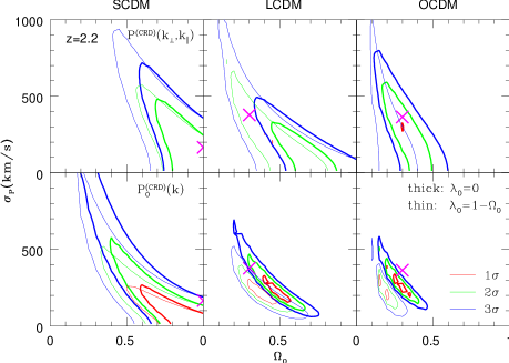
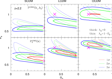
Fig. 19: The constraints on the $\mathchar 28938\relax_{0}$ - $\sigma_{P}$ plane derived from the $\chi^{2}$ analysis of simulation data at $z=2.2$. The upper panels are from $P^{(CRD)}(k_{s{\scriptscriptstyle\perp}},k_{s{\scriptscriptstyle\parallel}})$ with all the simulation particles ($N=256^{3}$), while the lower panels are from $P_{0}^{(CRD)}(k_{s})$ with $5\times 10^{4}$ randomly sampled particles. Thick and thin contours correspond to the results assuming $\lambda_{0}=0$ and $\lambda_{0}=1-\mathchar 28938\relax_{0}$, respectively. The crosses indicate the true values adopted in the simulation models. We assume Eq. (3.31) for the value of $\sigma_{8}$.

Fig. 20: The same as Fig. 20, but in the $\mathchar 28938\relax_{0}$ - $\sigma_{8}$ plane. We adopt an analytical fitting formula (Eq. (3.5)) for the value of $\sigma_{P}$.

Finally we compute the $\chi^{2}$ between the theoretical predictions (with nonlinear corrections) and the simulations by varying the parameters. The results are shown as contours in $\mathchar 28938\relax_{0}$ - $\sigma_{P}$ and $\mathchar 28938\relax_{0}$ - $\sigma_{8}$ planes in Figs. 20 and 20, respectively. In these figures, the upper and lower panels correspond to the analysis based on $P^{(CRD)}(k_{s{\scriptscriptstyle\perp}},k_{s{\scriptscriptstyle\parallel}})$ using all simulation particles ($N=256^{3}$) and $P_{0}^{(CRD)}(k_{s})$ using $5\times 10^{4}$ randomly sampled particles (one realization from each model in Table I). The $\chi^{2}$-fit is carried out in the range of $(2\pi/60)h{\rm Mpc}^{-1}<k_{\scriptscriptstyle\perp},k_{\scriptscriptstyle\parallel},k_{s}<(2\pi/20)h{\rm Mpc}^{-1}$.

In Fig. 20, we fix the value of $\sigma_{8}$ according to the fitting formula based on the following cluster abundances:[9]

$$\sigma_{8}=(0.54\pm 0.02)\times\left\{\begin{array}[]{ll}\mathchar 28938\relax_{0}^{-0.35-0.82\mathchar 28938\relax_{0}+0.55\mathchar 28938\relax_{0}^{2}}&\mbox{($\lambda_{0}=1-\mathchar 28938\relax_{0}$)},\\ \mathchar 28938\relax_{0}^{-0.28-0.91\mathchar 28938\relax_{0}+0.68\mathchar 28938\relax_{0}^{2}}&\mbox{($\lambda_{0}=0$)}.\end{array}\right.$$ (3.31)

In Fig. 20, we fix the value of $\sigma_{P}$ according to Eq. (14) in Ref. ?. Incidentally the cluster abundance constraints (3.31) are fairly orthogonal to our constraints from the redshift distortion.

The best-fit values for $\sigma_{P}$ and $\sigma_{8}$ in the above plots are slightly smaller than their true values (marked as crosses). This is related to the nonlinear velocity correction, as described above, and we can easily correct for this systematic effect by adopting a more appropriate model.[27] Therefore we conclude that it is feasible to break the degeneracy in the cosmological parameters by combining the cosmological redshift-space distortion in the future QSO samples with other cosmological tests, despite the fact that the present modeling of nonlinear effects is fairly empirical.

4 Conclusion

The present paper focuses on two important effects, the cosmological light-cone effect and redshift-space distortion, which have been largely ignored in previous discussions of clustering statistics. We have demonstrated that they play an important role in the analysis of the upcoming redshift surveys, particularly of high-redshift objects, as both cosmological signals and noise depending on specific aspects of the phenomena that one is interested in. We summarize our main conclusions here.

1. We derived an expression for the two-point correlation function properly defined on the light-cone hypersurface.[5] This expression is easily evaluated numerically when the underlying cosmological model is specified. With this, one can directly confront the resulting predictions with the observational data in a fairly straightforward manner.

2. The cosmological light-cone effect produces artificial scale-dependence and redshift-dependence on the higher-order moments[6] of redshift-space clustering of any cosmological objects.

3. In linear theory we formulated the cosmological redshift-space distortion[7] which induces an apparent anisotropy in two-point correlation functions, especially at high redshifts. Further detailed studies with N-body simulations[27] indicate that it is feasible to constrain the cosmological parameters from the future QSO samples via this effect even though the nonlinear evolution appreciably affects the linear theory predictions.

Apparently, the results described above should be regarded as the first attempts to raise the importance and basic features of these two cosmological effects. These results are still far from complete in the sense that there are many aspects which remain to be explored. We hope that this short review serves as a practical and useful introductory note for more detailed investigations in the future.

References

- [1] M. J. Geller and J. P. Huchra, Science 246 (1989), 897.
- [2] C. C. Steidel, K. L. Adelberger, M. Dickinson, M. Giavalisco, M. Pettini and M. Kellogg, Astrophys.J. 492 (1998), 428.
- [3] F. J. Carrera et al., MNRAS 299 (1998), 229.
- [4] B. J. Boyle, S. M. Croom, R. J. Smith, T. Shanks, L. Miller and N. Loaring, Phil.Trans.R.Soc.Lond.A (1998), in press (astro-ph/9805140).
- [5] K. Yamamoto and Y. Suto,Astrophys.J. 517 (1999), in press (astro-ph/9812486).
- [6] T. Matsubara, Y. Suto and I. Szapudi, Astrophys.J. 491 (1997), L1.
- [7] T. Matsubara and Y. Suto, Astrophys.J. 470 (1996), L1.
- [8] T. T. Nakamura, T. Matsubara and Y. Suto, Astrophys.J. 414 (1998), 13.
- [9] T. Kitayama and Y. Suto, Astrophys.J. 490 (1997), 557.
- [10] J. M. Bardeen, J. R. Bond, N. Kaiser and A. S. Szalay, Astrophys.J. 304 (1985), 15.
- [11] J. A. Peacock and S. J. Dodds, MNRAS 267 (1994), 1020.
- [12] J. A. Peacock and S. J. Dodds, MNRAS 280 (1996), L19.
- [13] J. N. Fry, Astrophys.J. 461 (1996), L65.
- [14] S. Wallington and R. Narayan, Astrophys.J. 403 (1993), 517.
- [15] T. T. Nakamura and Y. Suto, Prog. Theor. Phys. 97 (1997), 49.
- [16] F. La Franca, P. Andreani and S. Cristiani, Astrophys.J. 497 (1998), 529.
- [17] S. Matarrese, P. Coles, F. Lucchin and L. Moscardini, MNRAS 286 (1997), 115.
- [18] J. N. Fry, Astrophys.J. 277 (1984), L5.
- [19] F. R. Bouchet, R. Juszkiewicz, S. Colombi and R. Pellat, Astrophys.J. 394 (1992), L5.
- [20] B. Jain, H. J. Mo and S. D. M. White, MNRAS 276 (1995), L25.
- [21] C. Alcock and B. Paczyński, Nature 281 (1979), 358.
- [22] W. E. Ballinger, J. A. Peacock and A. F. Heavens, MNRAS 282 (1996), 877.
- [23] M. Davis and P. J. E. Peebles, Astrophys.J. 267 (1983), 465.
- [24] N. Kaiser, MNRAS 227 (1987), 1.
- [25] A. J. S. Hamilton, Astrophys.J. 385 (1992), L5.
- [26] A. J. S. Hamilton, to appear in the Proceedings of Ringberg Workshop on Large-Scale Structure, ed. D. Hamilton (1997), (astro-ph/9708102).
- [27] H. Magira, Y. P. Jing and Y. Suto (1999), in preparation
- [28] P. J. E. Peebles, Principles of Physical Cosmology (Princeton: Princeton Univ. Press, 1993).
- [29] J. E. Gunn and D. H. Weinberg, in Wide Field Spectroscopy and the Distant Universe, ed. S. J. Maddox and A. Araǵon-Salamanca (World Scientific, Singapore, 1995).
- [30] C. C. Dyer and R. C. Roeder, Astrophys.J. 180 (1973), L31.
- [31] K. Tomita, Prog. Theor. Phys. 100 (1998), 1.
- [32] Y. P. Jing and Y. Suto, Astrophys.J. 494 (1998), L5.
- [33] Y. P. Jing, Astrophys.J. 503 (1998), L9.
- [34] H. J. Mo, Y. P. Jing and G. Börner MNRAS 286 (1997), 979.
- [35] C. M. Baugh and G. Efstathiou MNRAS 267 (1994), 323.