Constraining the Role of SN Ia and SN II in Galaxy Groups by Spatially Resolved Analysis of ROSAT and ASCA Observations

Abstract

We present the results of modelling the distribution of gas properties in the galaxy groups HCG51, HCG62 and NGC5044, and in the poor cluster AWM7, using both ASCA SIS and ROSAT data. The spectral quality of the ASCA data allow the radial distribution in the abundances of several elements to be resolved. In all systems apart from HCG51, we see both central cooling flows, and a general decline in metal abundances with radius. The ratio of iron to alpha-element abundances varies significantly, and in comparison with theoretical supernova yields, indicates a significant contribution to the metal abundance of the intergalactic medium (IGM) from type Ia supernovae. This is seen both within the groups, and also throughout much of the cluster AWM7. The total energy input into the IGM from supernovae can be calculated from our results, and is typically 20-40 per cent of the thermal energy of the gas, mostly from SNe II. Our results support the idea that the SN II ejecta have been more widely distributed in the IGM, probably due to the action of galaxy winds, and the lower iron mass to light ratio in groups suggests that some of this enriched gas has been lost altogether from the shallower potential wells of the smaller systems.

1 Introduction

In this paper we present a study of the X-ray emission of galaxy groups using the good spatial resolution of the ROSAT PSPC in conjunction with the superior spectral capability of the ASCA SIS. For relatively cool systems like groups ($T_{\rm gas}\sim 1$ keV) the X-ray spectrum contains fairly strong signatures from a number of elements, and this allows us to investigate the distribution of heavy elements in the IGM. Making use of the different element yields of SN Ia and SN II, we can use this information to estimate the role of different types of SNe in enriching the IGM.

According to standard theories of the chemical evolution of early-type galaxies, their star formation will trigger a galactic wind, causing a loss of the enriched gas, which can be retained in the potentials of groups and clusters of galaxies (e.g. Renzini et al. 1993). In the first substantial study of cluster abundances using ASCA, Mushotzky et al. (1996) studied the integrated abundances of O, Ne, Si, S and Fe in four galaxy clusters, and concluded that the balance between $\alpha$-elements and iron favours the origin of most or all of the metals in SN II. More recently Fukazawa et al. (1998) have studied a much larger sample of 40 clusters, and have also discriminated out the central regions, which may be dominated by strong cooling flows. Their results indicate a significant contribution from SN Ia, in addition to SN II, especially in lower mass systems. In principle, ASCA can provide more detailed information on the spatial distribution of elements, rather than just on integrated abundances, and in the present study we exploit this capability. Our work complements that of Fukazawa et al. (1998), in that we derive detailed distributions for a small sample, where they study the integrated properties of a large collection of systems.

The distribution of metals in low mass clusters is of particular interest, since it is for such systems that the energetic effect of galaxy wind injection should have the greatest impact on the IGM. It appears that such effects have already been seen in the low beta values for groups and in a steepening of the $L:T$ relation at low temperatures (Ponman et al. 1996, Cavaliere, Menci & Tozzi 1997). These winds bring with them metals, so that a study of metal distributions places constraints on the history of wind injection. If, for example, winds have blown much of the SN II metals out of groups altogether, we would expect them to have lower iron mass to light ratios, and abundance ratios tilted more towards SN Ia than is the case in rich clusters. A study of the role of SN Ia and SN II in groups may also shed light on the mystery of iron production by ellipticals. The low abundance observed by ASCA in hot elliptical galaxy halos causes substantial difficulties for theoretical models of their chemical history (Arimoto et al. 1996).

For our study, we require good photon statistics, and have therefore picked three of the brightest X-ray groups. Two of these (HCG51 and HCG62) are compact groups, whilst the third (NGC5044) is a loose group. In practice (Mulchaey et al. 1996) the properties of compact groups appear to be similar to those of (X-ray bright) loose groups, and the distinction between the two may not be fundamental. For comparison, we also study a richer system, AWM7, (which should lie above the L:T break), but one which is still cool enough to allow ASCA to determine abundances for a range of elements.

In our study we use a 3-dimensional approach to modelling of ASCA data for these objects, and we also compare our results for HCG62 with an independent 3-dimensional analysis of ROSAT PSPC data using the Birmingham cluster fitting package. $H_{\rm o}=50$ km s^-1 Mpc^-1 is assumed throughout the paper. Unless clearly stated otherwise, all errors quoted in this paper correspond to 90 per cent confidence level.

2 Analysis

In the analysis of ASCA data, presented below, we used data from the SIS0 and SIS1 detectors, which provide energy resolution of $\sim$75 eV at 1.5 keV. A detailed description of the ASCA observatory as well as the SIS detectors can be found in Tanaka, Inoue & Holt (1994) and Burke et al. (1991). Standard data screening was carried out using FTOOLS version 3.6. The effect of the broad ASCA PSF was simulated, as described in Finoguenov et al. (1998), and the analysis allows for the projection onto the sky of the three-dimensional distribution of emitting gas. In this approach, we use ROSAT data to derive the source’s surface brightness profile, which is represented by a one or two component “$\beta$-model” (Jones & Forman 1984). This is used to construct a three-dimensional model which is projected onto the regions of the SIS detectors chosen for extracting spectra. The thickness of the shells in our “onion peeling” technique is chosen to avoid any drastic variation of the temperature ($T$) and metallicity ($Z$) within one bin, which would invalidate our single component spectral modelling.

GIS data were not used in our analysis due to their lower energy resolution and uncertainties in calibration below 2 keV. Our technique for analyzing the ASCA data restricts us to usage of ASCA pointings with less than $25$^′ offset from the source centre, due to the similar restrictions in calibration data for the ASCA ray-traced PSF and the importance of accounting for the stray light at larger offset angles (cf Ezawa et al. 1997). In practice this restriction is of importance only for the AWM7 analysis.

All fits are based on the $\chi^{2}$ criterion. No energy rebinning is done, but a special error calculation was introduced following Churazov et al. (1996), to avoid ill effects from small numbers of counts. ROSAT (Truemper 1983) images of all the sources were used as an input for ASCA data modelling. For imaging analysis of the ROSAT data we used the software described in Snowden et al. (1994) and references therein. For the ROSAT/PSPC observation of HCG62 we also performed an independent three-dimensional modelling analysis using the Birmingham cluster fitting package (Eyles et al. 1991) for comparison with our ASCA results.

In our approach to the analysis of ASCA data, where all the derived spectra are fitted simultaneously, and where correlation between different regions is rather high, a simple minimization of $\chi^{2}$ proves to be an ill-posed task (Press et al. 1992, p.795). The best fitting model displays large fluctuations in temperature and metallicity profiles as it attempts to fit noise in the data. The solution to this problem is to accept a much smoother model which gives an acceptable fit (rather than the very best fit) to the data. This is achieved through regularization, which applies a prejudice in favour of some measure of smoothness (Press et al. 1992, p.801). We have made a default assumption that a linear function (of log radius) is a good representation of our temperature and abundance distributions. Departures from linearity are quantified by calculating the second derivative of the distribution, which is squared and added to the $\chi^{2}$ statistic.

In using any regularization technique, special attention should be paid to the balance between maximizing the likelihood and optimizing the smoothness of the solution. This is traditionally done by introducing a weighting constant into the regularization term. We set this constant so as to obtain a solution which lies within the 68 per cent confidence region surrounding the minimum $\chi^{2}$ (i.e. unsmoothed) solution in the n-parameter space. The allowed offset in $\chi^{2}$ was evaluated using the prescription of Lampton et al. (1976).

Table 2: Optical characteristics.

Name	D	$L_{B,cD}$	$L_{B}^{{}^{a}}$	$R_{L_{B}}$	$R_{v}$	$R_{c}$
	Mpc	$10^{11}$$L_{\odot}$	$10^{11}$$L_{\odot}$	Mpc	Mpc	kpc
HCG62	82		0.95	1.09	1.09	27
HCG51	155		2.8	1.19	1.19	59
NGC5044	54	0.68	1.6b	0.5	1.19	180
AWM7	106	1.9	13.2b	1.84	1.89	220

^a  blue luminosity of early-type member galaxies

^b  Assuming 30% contribution of spirals to a total blue luminosity

Since regularization introduces a dependence of the measurement in a given spatial bin on that from the adjacent bins (due to the operation of the prejudice towards smoothness), presenting formal error bars at every point is misleading. Instead, more valid representation is an area of possible parameter variation with radius. We choose a confidence level of 90 per cent for these representations. Thus, points will represent the best-fit solution, while a shaded zone will mark the area of solutions allowable within the chosen confidence level.

The analysis presented in this paper differs from previous work on these objects (e.g.  Fukazawa et al. 1996), which have generally ignored the effects of projection and PSF blurring. Since the PSF is energy-dependent, simplified analyses can give misleading results (Takahashi et al. 1995). For relatively cool systems, like the groups studied here, there is an additional effect connected with the possible presence of temperature gradients. Determination of iron abundance at temperatures $\sim 1$ keV is based on L-shell lines. Individual lines in the L-shell complex are unresolved by ASCA, and merge into a broad peak with a position which is sensitive to temperature. If the temperature structure is not resolved and a mean temperature is used, then iron abundance will be underestimated by a significant factor, because there will be some mismatch between peak positions.

To illustrate this effect, we simulate an SIS spectrum using the characteristics of the HCG62 data (ARF file, response file, duration of the observation). The model involves a mix of 2 temperatures: 0.7 keV and 1.2 keV, with both components having equal emission measures (a “norm” parameter of $2.\times 10^{-4}$ in XSPEC, typical for the groups analyzed here) and all element abundances equal to 0.5 solar. MEKAL plasma code is used throughout this illustration. When the simulated data are fitted with a single-temperature model we find $kT=0.823\pm 0.026$, Mg$=0.18\pm 0.14$, Si$=0.11\pm 0.08$ and Fe$=0.19\pm 0.03$ with emission measure normalization being $7.3\pm 1.6\times 10^{-4}$. Hence the abundances are underestimated, and the emission measure overestimated. Such effects may compromise any study in which temperature structure is not resolved. This is likely to apply even to the current study, in central cooling flows, where steep temperature gradients and multiphase gas may be present.

In all our spectral modelling, we use the MEKAL model (Mewe et al. 1985, Mewe and Kaastra 1995, Liedahl et al. 1995). Abundances of He and C were set to solar values as in Anders & Grevesse (1989), where element number abundances relative to hydrogen are (85.1, 12.3, 3.8, 3.55, 1.62, 0.36, 0.229, 4.68, 0.179)$\times 10^{-5}$ for O,Ne,Mg,Si,S,Ar,Ca,Fe,Ni, respectively. In the case of the three groups, only Mg, Si and Fe features are clearly seen in the data. We cut the ASCA spectra above 2.2 keV, so S and Ar features are outside the range of measurements, and arrange elements into four groups, based on their production history: O and Ne; Mg; Si, S and Ar; and Ca, Fe and Ni. The analysis yields meaningful values for abundances of Mg, Si and Fe. O and Ne results are not derived for groups, and we do not group O with other elements, like Si, in order to avoid possible effects from ASCA calibration uncertainties at low energies. For the same reason, we do not present any results for O abundance in the analysis below.

Our choice of the MEKAL plasma code leads to systematically lower temperatures (at the 10–20 per cent level) in the temperature range below 1 keV, compared to the Raymond-Smith code (Raymond et al. 1977). There have been made several attempts to quantify the uncertainty in the Fe abundances determined using L-shell line emission. It was shown in a study by Matsushita (1998), that if Fe abundance is decoupled from the other heavy elements, the range in Fe abundances derived from different codes is 20 per cent. We therefore add a systematic error of $\pm 10$ per cent at 1$\sigma$ confidence level to the derived Fe abundances.

Figure 2: Spatially resolved ASCA SIS spectra of (a) NGC5044, at radii of 0^′–2^′–8^′–16^′  from bottom to top plots, (b) HCG62, at radii 0^′–1.5^′–8^′–16^′  from bottom to top plots, (c) HCG51, at radii 0^′–2^′–6^′ from bottom to top plots, and (d) AWM7, at radii 0^′–3^′–10^′–25^′ from bottom to top plots). Y-axis values are arbitrarily scaled for clarity.

Using the 0.7–7.0 keV band in the case of AWM7, we fit all major elements separately, except for the grouping of Ca and Ni with Fe, and obtain useful results for the abundances of Ne, Si, S and Fe. A special comment should be made on Mg. It has been noted (Mushotzky et al. 1996) that in the case of cluster emission, this may be affected by the proximity of the poorly understood 4–2 transition lines of iron, which cannot be resolved with ASCA SIS. This problem affects our AWM7 data, however at the lower temperatures of groups, the relevant Fe L-shell lines are weak and hence uncertainties in modelling them has little impact on the abundance of Mg determined. Spatially resolved ASCA SIS spectra obtained for the sources in our study are illustrated in Fig.2.

3 Results

In this section we present the details of the analysis and results for each individual system analyzed. Optical data, which will be used for comparison with the X-ray results, are provided in Table 2. Columns in this table are: (1) system name, (2) adopted distance in Mpc, (3) B-band luminosity of the central galaxy for the two systems with dominant central galaxies, (4) total luminosity of early-type galaxies, and (5) radius within which this optical luminosity is measured. Optical data were taken from Hickson et al. (1992) for HCG51 and HCG62, David et al. (1994) for NGC5044 and Beers et al. (1984) for AWM7. For the latter object we adopt a spiral fraction of 0.3, average for clusters, since no measurements are available to date, however our results are insensitive to this choice. The remaining columns give: (6) virial radius calculated using a formula derived from simulations by Navarro et al. (1994), $R_{virial}=1.04T_{keV}^{0.5}(H_{o}/50)^{-1}$ Mpc, where T is luminosity weighted X-ray temperature (excluding the cooling flow), and (7) optical core radius taken from Hickson et al. (1992), Ferguson & Sandage (1990) and Dell’Antonio et al. (1995).

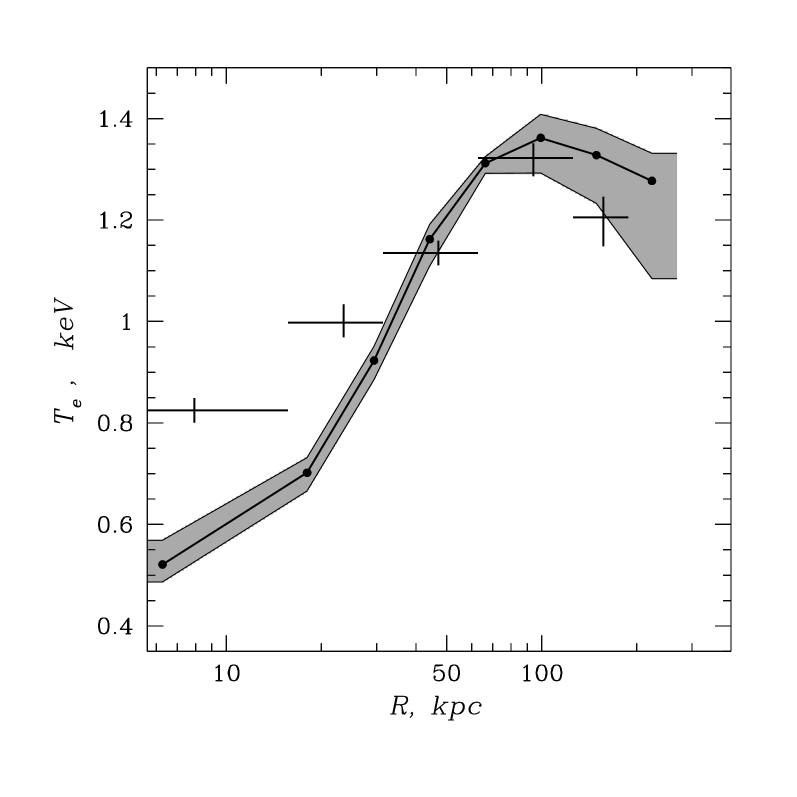
Figure 4: Temperature profile of NGC5044. ROSAT PSPC points are represented by black crosses, solid line represents the best-fit curve describing ASCA results with filled circles indicating the spatial binning used. Shaded zone around the best fit curve denotes the 90 per cent confidence area.

Masses of gas and various metals derived in the X-ray analysis discussed in the remainder of this section are collected together in Table 4. The radius within which these masses are derived is listed in the second column of the table. All error intervals are quoted at 90 per cent confidence level. Limits on masses are obtained by integrating the corresponding lower and upper 90 per cent boundary on the abundance estimation and adding an error on gas mass estimation in squared.

3.1 NGC5044

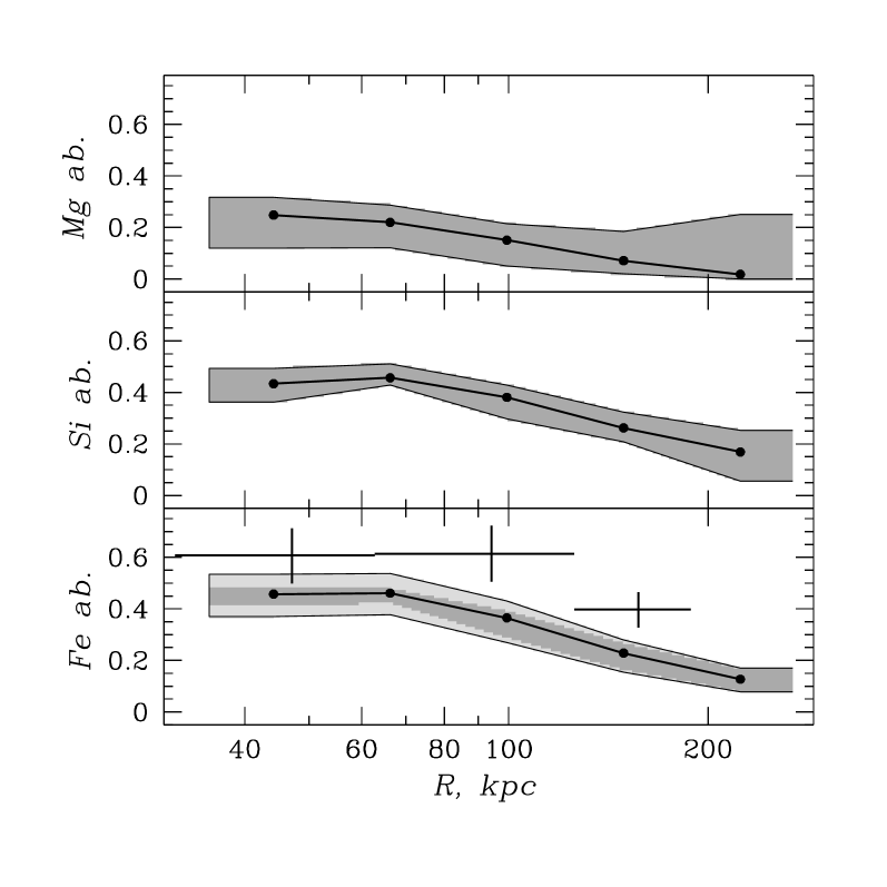
Figure 6: Element abundances in NGC5044. ROSAT PSPC points are represented by black crosses, solid line represents the best-fit curve describing ASCA results with filled circles indicating the spatial binning used. Shaded zone around the best fit curve denotes the 90 per cent confidence area. Light shaded zone on the Fe abundance plot indicates the contribution to this zone of a 10 per cent systematic error, as discussed in the text.

Table 4: Cumulated gas and metal masses.

Name	$R_{out}$	$M_{gas}$	$M_{Fe}$	$M_{Si}$	$M_{Mg}$	$M_{S}$	$M_{Ne}$
	kpc	$10^{12}$ $M_{\odot}$	$10^{8}$ $M_{\odot}$	$10^{8}$ $M_{\odot}$	$10^{8}$ $M_{\odot}$	$10^{8}$ $M_{\odot}$	$10^{8}$ $M_{\odot}$
HCG 62	410	1.656 (1.56–1.76)	3.82 (1.8–5.8)	2.24 (0.5–3.4)	0.23 (0.1–3.8)	—	—
HCG 51	270	0.609 (0.56–0.65)	4.05 (3.0–5.1)	1.99 (1.6–2.3)	1.59 (0.6–1.9)	—	—
NGC 5044	270	0.965 (0.92–1.00)	4.09 (2.7–4.9)	1.75 (1.1–2.2)	0.49 (0.2–1.5)	—	—
AWM 7	790	21.34 (21.1–21.5)	95.2 (74–115)	75.7 (61–89)	—	9.4 (1.3–18)	113 (55–149)

The galaxy group NGC5044 is well-suited for spatially resolved spectroscopy, it is nearby ($z=0.0087$), and shows bright and fairly symmetrical diffuse X-ray emission (David et al.  1994). The group has a dominant central elliptical surrounded by many smaller galaxies. From analysis of ROSAT PSPC observations (David et al.  1994) the diffuse X-ray emission of this object extends to $\sim 20$^′ radius (1^′ corresponds to 15.7 kpc). A strong temperature gradient is observed in the centre of the diffuse emission, pointing to the presence of a cooling flow. Deprojection gives a central temperature $\sim$0.8 keV. The mass accretion rate is significant only within the central 40 kpc and amounts to $\sim 10$$M_{\odot}$ per year. The gas cooling time at $r\approx 40$ kpc is $10^{9}$ yr.

ASCA observations of NGC5044 were carried out during June 20–21 1993. We used a representation of the surface brightness profile from ROSAT PSPC data given by a $\beta$-model with parameters $\beta=0.51$, $r_{a}=10.6$ kpc, obtained from our analysis of ROSAT PSPC data in the 0–40^′ region, excluding point sources and a “cooling wake”, found by David et al.  (1994). To compare with our ASCA results, we carried out an identical 3-dimensional spectral analysis with ROSAT PSPC data.

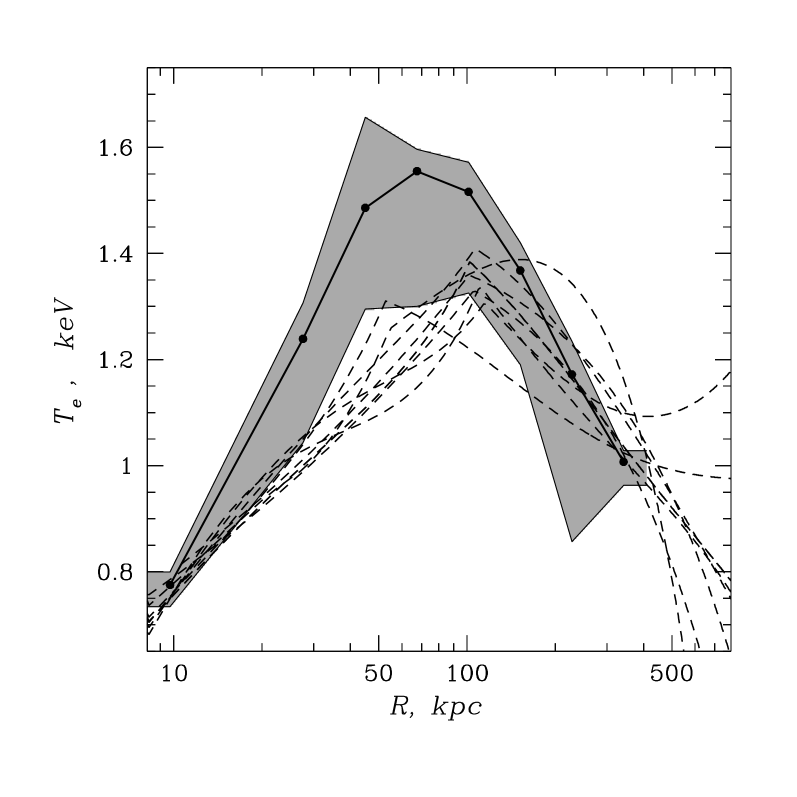
Figure 8: Temperature profile of HCG62. Results of a three-dimensional analysis of ROSAT PSPC data, fitting a variety of models to the data, are shown in dashed lines. Filled circles indicating the spatial binning and the shaded area showing the 90 per cent confidence level area around the best fit (solid line) present the ASCA SIS results.

In Fig.4 we present a temperature profile of NGC5044. ROSAT PSPC points are represented by black crosses, solid line represents the best-fit curve describing ASCA results with filled circles indicating the spatial binning used. Shaded zone around the best fit curve denotes 90 per cent confidence area. The ASCA data confirm a pronounced cooling flow at the centre with a temperature drop from 100 kpc to 10 kpc by a factor of two. ASCA and ROSAT results agree at radii exceeding 30 kpc, with the disagreement at small radii indicating the presence of complex temperature structure in the central cooling flow. Our results agree well with the previous finding of David et al.  (1994) that between 60 and 250 kpc the gas is nearly isothermal.

Element abundance profiles are shown in Fig.6. (We exclude the cooling region, where abundance results may be unreliable.) A significant decrease with radius is observed, and we see for the first time that this applies to Mg and Si in a similar way to Fe. The abundance of iron determined from ROSAT data (grey points) also shows a decrease with radius. The ASCA abundances drop from 0.3, 0.5 and 0.5 solar at $r=40$ kpc to near 0.0, 0.2 and 0.1 solar by $r=200$ kpc for Mg, Si and Fe, respectively. Shown errors on Fe abundance are dominated by the assumed systematic uncertainty in modelling.

3.2 HCG62

HCG62, is a compact group, taken from the catalogue of Hickson (1982), which was compiled by locating compact configurations of galaxies on the Palomar All Sky Survey in the E-band. HCG62 is the most luminous of the Hickson groups in the X-ray (Ponman et al. , 1996) and an analysis of the ROSAT PSPC data for HCG62 is presented in Ponman & Bertram (1993). The ASCA SIS observation analyzed here was carried out on January 14 1994.

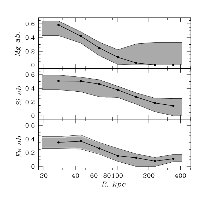
Figure 10: Mg, Si and Fe abundance profiles for HCG62 from ASCA data. Data representation is similar to Fig.6.

For our analysis we adopt a distance of 82 Mpc, which corresponds to a scale 1^′$=$ 23.9 kpc. The X-ray surface brightness profile is characterized by a double $\beta$-model fitted to the ROSAT PSPC data in the $r=0-20$ ^′ interval. The derived parameters of ($\beta$, $r_{a}$) are (0.66, 10.3 kpc) and (0.30, 52 kpc). Results of our analysis of ASCA SIS data were then compared with the results of three-dimensional modelling of the ROSAT PSPC data using the Birmingham cluster fitting package (Eyles et al. 1991), which also allows for the effects of projection and energy dependent PSF blurring, but adopts simple analytical models to represent the continuous gas density and temperature distributions, rather than the regularised discrete distributions employed in our ASCA analysis.

In Fig.8 we compare the temperature distributions derived from the ASCA and ROSAT data using these two different analysis systems. In the case of the ROSAT data, a variety of different models for the temperature distribution have been fitted to the data, to give an indication of the model dependence of the results. In general the two sets of results show an encouraging level of agreement. The temperature profile is characterized by cooling at the centre and a gradual decrease toward the edge of the group.

The element distributions derived from the ASCA analysis, presented in Fig.10, show strong gradients of Mg, Si and Fe abundance, in the same sense as NGC5044. At $r=20$ kpc Mg and Si abundance are 0.4 solar, Fe is 0.3 solar. All decline to $\sim$0.1 solar by a radius of 400 kpc. The Fe abundance gradient implied by ROSAT data matches the ASCA data in the outer parts, but rises to $\sim$0.6 solar at 40 kpc, although this difference near the centre is still within the combined 90% errors from both analyses.

3.3 HCG51

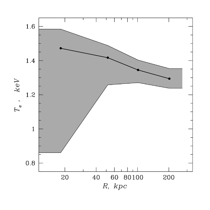
Figure 12: Temperature profile of HCG51, derived from ASCA SIS data. The best-fit curve does not indicate the presence of the cooling flow in the data, although the uncertainty in the parameter estimation is large for the inner points.

From results of the compact group survey of Ponman et al.  (1996), HCG51 is one of the most X-ray luminous of the compact groups. Apart from a short observation in the ROSAT All Sky Survey, the group was never observed by the ROSAT PSPC. However a 25 ksec observation was obtained in May 1995, and has been reduced using the Starlink ASTERIX analysis system, to derive a surface brightness profile for use in the ASCA data modelling procedure.

Diffuse emission is centered on the brightest elliptical galaxy in the group, and is detected in the HRI data out to 6^′ from the group centre. An adequate description of the profile in terms of $\beta$-models requires the introduction of a second component giving parameters ($\beta$, $r_{a}$) equal to (11.1, 33.2 kpc) and (0.30, 81 kpc).

ASCA observations of HCG51 were carried out on June 3–5 1994 using two-CCD mode for the SIS. We adopt a distance of 154.7 Mpc to HCG51, which gives a scale 1^′$=$45 kpc.

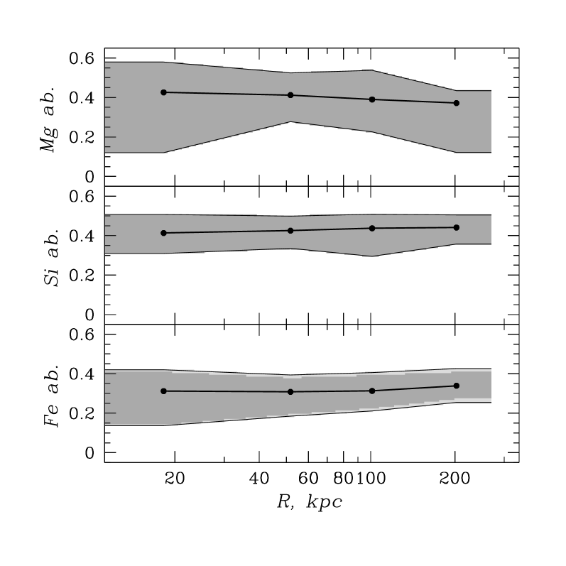
Figure 14: Mg, Si and Fe abundance profiles in HCG51 derived from ASCA SIS data (data representation is similar to Fig.6). No significant gradients are seen.

The derived temperature and abundance profiles are presented in Fig.12 and 14. In contrast to the other systems studied here, HCG51 does not show pronounced signs of a cooling flow. The temperature is $\sim 1.35$ keV, with some indication of a gentle decline with radius. Nevertheless, considering the confidence area for temperature estimation, it is possible to fit in the central cooling zone. The derived abundances of Mg, Si and Fe do not show any significant variation with radius. The lack of pronounced central cooling and the flat abundance profiles (contrasting with strong gradients in the other systems) strongly suggest that recent gas mixing has taken place in HCG51.

3.4 AWM7

ASCA SIS observations of AWM7 were obtained during August 7–8 1993 and February 10–12 1994. We adopt a distance to AWM7 of 105.6 Mpc, so that 1^′$=$31 kpc. A surface brightness model was taken from the work of Neumann & Boehringer (1995), giving values of the parameters ($\beta$, $r_{a}$) in the two $\beta$-model approximation of (0.25, 5 kpc) and (0.53, 102 kpc). The relative normalization of the components was chosen to give a central density ratio of 2, as obtained by Neumann & Boehringer (1995).

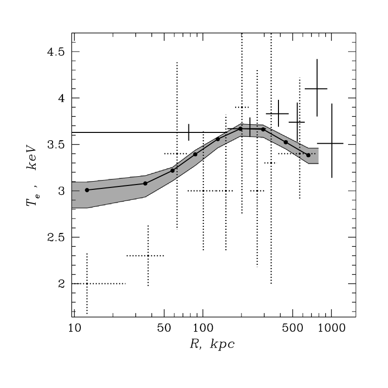
Figure 16: Temperature profile of AWM7. Filled circles represent best fit to our ASCA SIS data with shaded area showing the 90 per cent confidence level. Crosses, denoted with a dotted line represent ROSAT/PSPC data from Neumann & Boehringer (1995), solid black crosses denote the results of Ezawa et al. (1997). All confidence intervals on the plot are given at 90 per cent confidence.

In Fig.16 we compare the temperature profile derived here from ASCA data with the previous findings of Neumann & Boehringer (1995) and also from an annular spectral analysis (neglecting projection effects) of ASCA data by Ezawa et al. (1997). The latter authors have extended their analysis to larger radii than the present work, due to a more detailed treatment of stray light effects, but did not apply any regularization, resulting in rather coarse spatial resolution. The three analyses are in broad agreement apart from near the centre, where ROSAT data show the strongest cooling flow, while the analysis of Ezawa et al. (1997) does not reveal any temperature decrease at all. Our temperature profile is intermediate, but disagrees significantly with the ROSAT results only at $r<50$ kpc, indicating the probable presence of a multi-phase cooling flow, as discussed by Markevitch & Vikhlinin (1997).

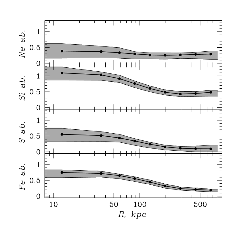
Figure 18: Abundances of Ne, Si, S and Fe in AWM7, obtained from ASCA SIS data (data representation is similar to Fig.6). An initial abundance decrease is followed by flattening at a radius of $\sim$200 kpc.

In Fig.18 we present abundance profiles derived for Ne, Si, S and Fe. All abundances show a decrease with radius which, with the possible exception of Fe, flattens off outside 200 kpc. Central values are 0.4, 1.1, 0.6 and 0.7 solar, respectively, dropping at $r=$800 kpc to 0.3, 0.5, 0.1 and 0.2 solar. The strong cooling flow may be expected to affect derived abundances in the inner regions, though the effects will be less severe than in cooler systems. To gauge these effects we have fitted spectra from the central 3^′ with a model including a cooling flow component. The inclusion of such a component has a negligible effect on the derived Fe abundance (which is largely based on the Fe K line for this system), whilst abundances of Si and S rise by $\sim 35$ per cent, and Ne is poorly constrained. Hence allowing for the effects of central cooling is only likely to increase abundance gradients, and amplify the contribution of $\alpha$-elements in the centre of the cluster, which we discuss below.

To investigate the systematic effects of ASCA PSF calibration uncertainties, we explored the effects of varying the spatial binning of the data. The conclusion we derived from these exercises is that the detected abundance gradients are robust, exception for the central excess of sulphur in AWM7, which was found to be lower with coarser binning.

4 Discussion

Using the above results for the abundance distributions of iron and $\alpha$-elements in these systems, we now proceed to examine the contributions from SNe II and SNe Ia to the metal enrichment. We also derive the iron mass to light ratio (IMLR) for the intracluster gas in each system, which gives clues about overall metal production and loss, and given our derived supernova rates we evaluate the importance of energy injection by SNe. Finally, we consider our results in the context of hierarchical clustering models.

4.1 Roles of different types of SNe in chemical enrichment of the IGM

The heavy elements liberated in type Ia and type II supernovae differ markedly in the ratio of iron to the elements (O, Ne, Mg, Si and S) generated by the alpha-process. For example, the Si/Fe abundance ratio is at least 4 times higher in the ejecta of SN II, compared to SN Ia. Unfortunately, the complexity of the theory of SN II explosions leads to a substantial uncertainty in SN II yields between different models. First attempts to confront the abundance measurements in clusters with theoretical predictions were made by Loewenstein & Mushotzky (1996). Their conclusion was that for some models one doesn’t need any SN Ia to reproduce the observed element ratios. They also found that none of the models they considered could self-consistently explain all the element ratios observed.

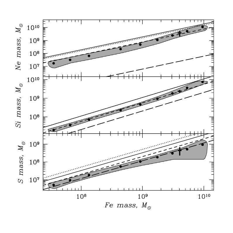
Figure 20: Ne, Si and S mass vs Fe mass in AWM7. Crosses represent ASCA SIS data from Mu96. Filled circles indicate our best-fit solution with shaded regions denoting the 90 per cent confidence intervals. The long-dashed line shows the theoretical mass ratio for SN Ia yield (TNH93 model), whilst SN II yields from the compilation of Gibson et al. (1997) are shown by solid and dotted lines denoting a choice of T95 and W95 yields, respectively. (These coincide in the case of Si.) The dashed line represents a 60 per cent contribution of SN Ia to the iron enrichment, using T95 yields for SN II.

Turning to our observation of AWM7 – this is one of the objects studied by Loewenstein & Mushotzky (1996, LM96), based on the measurements of Mushotzky et al. (1996, Mu96), but we are able to build a more detailed picture, since we have resolved the radial element distributions. SN II yields are taken from the recent work of Gibson et al. (1997), where an attempt was made to put different theoretical predictions onto the same mass grid for more direct comparison. We use models T95 and W95(A,Z_⊙), from Gibson et al. (1997), which are both integrated over a Salpeter IMF. SN Ia yields are subject to much less uncertainty, and are taken from Thielemann et al. (1993, TNH93). Average stellar yields for Ne, Mg, Si, S, Fe in solar masses are 0.232, 0.118, 0.133, 0.040, 0.121 for the T95 model; 0.181, 0.065, 0.124, 0.058, 0.113 for the W95 model; 0.005, 0.009, 0.158, 0.086, 0.744 for the TNH93 model.

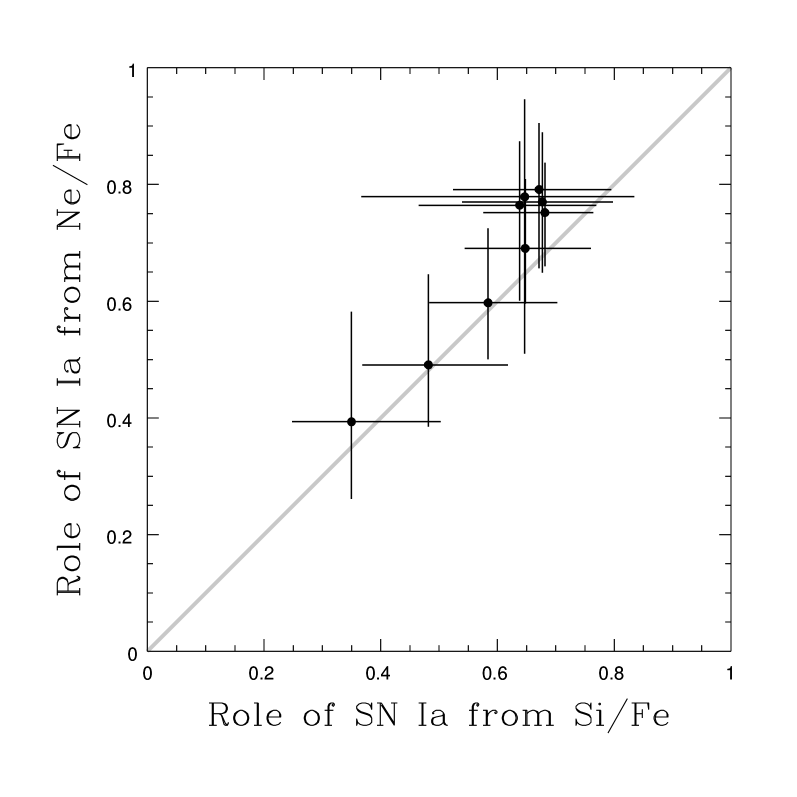
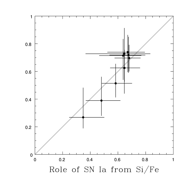
Figure 22: Input of SN Ia into the iron mass, calculated from Si/Fe and Ne/Fe ratios, assuming T95 (left panel ) and W95 (right panel) yields for SN II. Points correspond to measurements at different radii in AWM7. Error bars are 1$\sigma$, and the points are not independent due to regularization.

In Fig.20 we consider the behaviour of the cumulative masses of $\alpha$-elements plotted against the cumulative mass of iron. The shaded zone represents the 90 per cent confidence area for deviation from either parameter, so the form of the shaded area at the boundary points has an elliptical form. The element ratios predicted for SN Ia and the chosen models of SN II are shown by straight lines. In addition we plot a line corresponding to a 60 per cent contribution of SN Ia to the iron mass, calculated using the T95 model for SN II yields and the TNH93 model for SN Ia yields. Also marked are the results of Mu96, which agree with our values well at comparable radii. Note that Si/Fe (and Ne/Fe) is lower than the Mu96 value at smaller radii, but continues to rise towards SN II-like ratios at larger radii.

An anomaly immediately apparent in Fig.20, is that whilst Ne and Si masses show similar behaviour in the SN Ia – SN II reference frame, the S/Fe ratio is approximately constant through the cluster. The anomalous behaviour of the S/Fe ratio was also noted in integrated spectra by Mu96. We note that not only the absolute value, but also the trend in the S abundance is anomalous. The observed S/Fe ratio is consistent with 100 per cent Fe production by SNe Ia throughout the cluster, while from other elements it varies from 70 per cent down to 30 per cent, from inner to outer radial points. Such behaviour appears to imply that the SN II model yields for sulphur are incorrect or that the observed abundance is modified by some additional physical process.

Leaving sulphur aside as unreliable, we can derive independent estimates of the fraction of the iron which is contributed by SN Ia from the Si/Fe and Ne/Fe ratios, using a given pair of models for the SN Ia and SN II yields. This can be used as a test of the consistency of the models. In Fig.22 we compare the results for AWM7 using the T95 and W95 models for SN II (the TNH93 model yields are adopted for SN Ia in each case). Both models appear acceptable in this case. For comparison, the SN II model of Thielemann et al. (1996; yields for Fe and Si are 0.11 and 0.08 in solar masses), which LM96 note can give a reasonable match to most of their integrated abundances without any SN Ia contribution, fails to explain the high Si/Fe ratio which we observe at the outer radii in our AWM7 analysis.

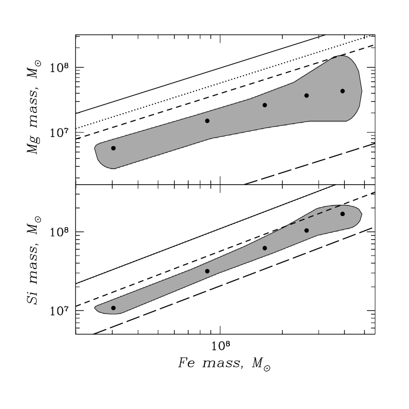
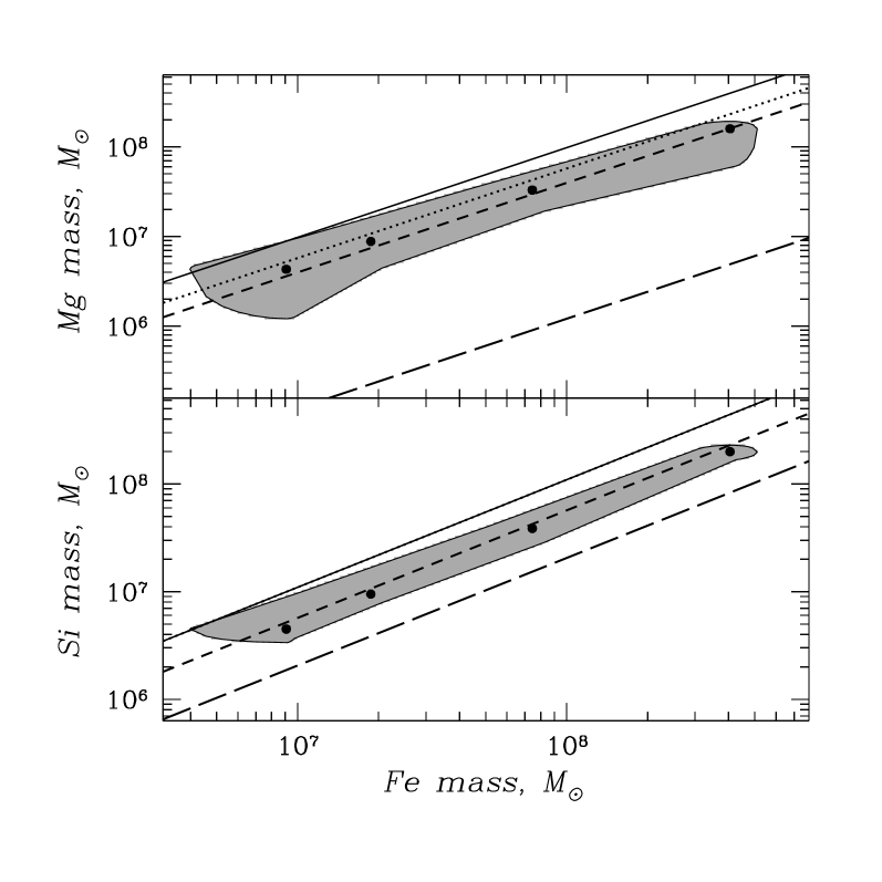
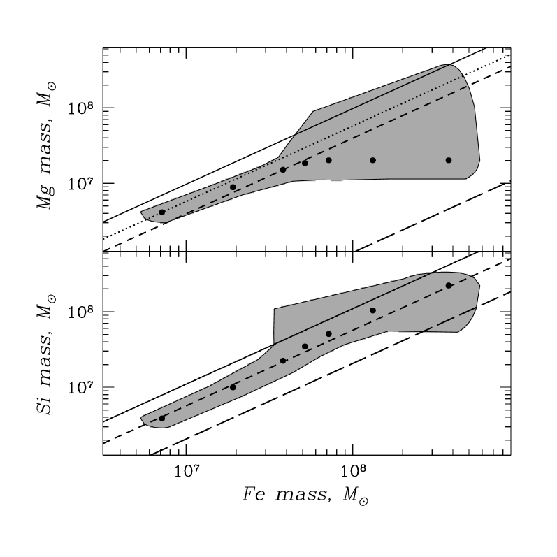
Figure 24: Mg and Si mass vs Fe mass in NGC5044 (left), HCG51 (center) and HCG62 (right). Line coding for the theoretical SNe yields and data representation is similar to Fig.20.

Our data on the abundance ratios in the groups are presented in Fig.24. Again, these ratios indicate significant contributions from both SN Ia and SN II, but the variation of the element ratios with radius is less pronounced than in AWM7. The role of SNe Ia in iron production is the strongest in NGC5044, where they provide $75\;(54-98)$ per cent of the iron within the region analyzed, while in HCG62 and HCG51 the corresponding values are somewhat lower and amount to $48\;(10-100)$ and $68\;(40-95)$ per cent, respectively. Consistency between the estimates of the SN Ia contribution from Si/Fe and Mg/Fe is somewhat better for the T95 model than for W95. But both models are acceptable within the errors, as is illustrated in Fig.26.

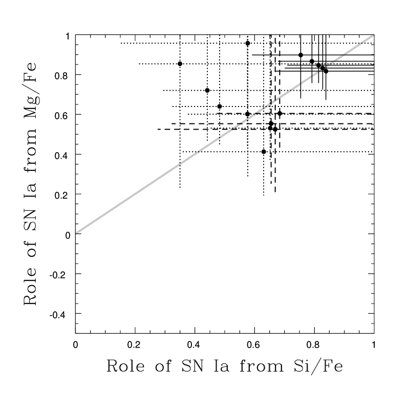
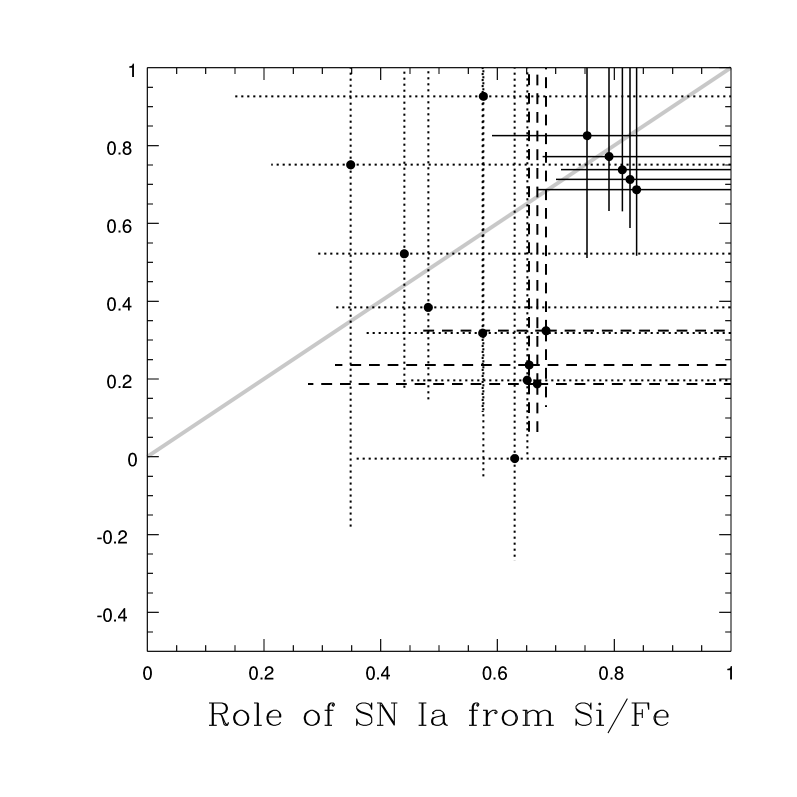
Figure 26: Input of SN Ia into the iron mass, calculated from Si/Fe and Mg/Fe ratios, assuming T95 (left panel) and W95 (right panel) yields for SN II. Solid line denotes NGC5044 data, dashed – HCG51 and dotted – HCG62. Error bars are 1$\sigma$, and the points are not independent due to regularization.

The need for a significant SN Ia contribution to explain the abundance ratios in the systems we study has interesting implications for the debate on the chemical evolution of elliptical galaxies. In particular, one of the options discussed by Arimoto et al. (1996) to account for the apparently low abundances seen in the hot gas within ellipticals, was that the SN Ia rate has always been low. This option is ruled out by our results, and also by the findings of Fukazawa et al. (1998).

4.2 Iron profiles for SN Ia and SN II

The iron abundance gradients seen in most of our systems show that the IGM is not completely mixed. In addition to Fe, abundance gradients are detected for $\alpha$-elements: Mg and Si in HCG62 and NGC5044, and Ne, Si and S in AWM7. As discussed above in relation to AWM7, the balance between the contribution of different SNe types could be a variable function of radius. To explore this further, we use the ratio of $\alpha$-elements to iron as a function of radius to decompose the iron profile into radially varying contributions from SN Ia and SN II. The situation is complicated by the likelihood that there will also be some contamination of the IGM by metals released within galaxies by stellar mass loss. Assuming that most of the metals in the IGM are liberated from early-type galaxies (Arnaud et al.  1992) the abundance ratios of such winds would be similar to that of SN II, so this contribution will effectively be included in the SN II component in our decomposition. As we will see in the next section, the stellar wind contribution, if it can escape from galaxies, may be significant, but should not be a dominant component in the observed mass of metals.

For our decomposition of the iron profile into the two major SN types, we use the Si and Fe abundance measurements and the yields of T95. This approach has the advantages that Si and Fe are measured for all systems studied here, the Si abundance is the best constrained of the $\alpha$-elements, and the spread in the Si/Fe yields between the T95 model and the various models of W95 is small. This provides more confidence in the derived results. In Fig.28 we present the iron profile attributed to SN II (upper panel) and SN Ia (lower panel) for all each of our systems apart from HCG51, which has essentially uniform abundances of all elements, as was shown earlier.

The main feature seen in Fig.28 is the strong central concentration of the SN Ia iron profile, in comparison to a flatter distribution in the SN II iron contribution. Note that the fact that the Si/Fe ratio varies significantly with radius in three of these systems implies the need for at least two different sources of enrichment, irrespective of the details of specific models for supernova yields.

To analyze the central excess in the SNe Ia contribution, we fitted a King profile. The values of the fitted core radii are 60 (27–121) kpc for HCG62, 117 (65–213) kpc for NGC5044 and 171 (104–262) kpc for AWM7, which compares with their corresponding optical core radii of 27, 180 and 230 kpc. We return to the broad similarity between these core radii below.

Figure 28: Iron profiles decomposed into the two major types of SNe. Solid lines represent AWM7 data, dashed line – NGC5044, dotted – HCG62. Results for HCG51 are not shown since abundances show no significant variations.

If it is assumed that SN II ejecta escape primarily from early-type galaxies, where they are generated by an initial massive burst of star formation accompanying the birth of these galaxies (e.g. Matthews 1989), or by subsequent bursts triggered by galaxy merging ( Schweizer & Seitzer 1992), then their injection will be closely associated with active star formation, and take place via highly energetic winds. The fact that the SN II products are so widely distributed, in contrast to the SN Ia ejecta, which are expected to be released over a much longer timescale after star formation, suggests that the bulk of the SN II activity occurred early in the life of the system. This is consistent with the picture of Ponman, Cannon & Navarro (1999), who find that most of the supernova energy injection must actually precede the collapse of groups and clusters in order to account for the magnitude of the rise seen in the entropy of the gas.

The total level of Fe attributed to SN II products indicates the ability of the system to retain SN II-driven winds. Groups are characterized by a small spread around a value of 0.1 solar, with average values of $0.07\pm 0.02$ for NGC5044 and $0.11\pm 0.03$ for HCG62, however the SN II contribution in both systems drops below 0.05 solar at large radii. The SN II contribution to the well mixed IGM in HCG51 is equal to $0.10\pm 0.02$, within the region analyzed.

In AWM7, the SN II contribution to the Fe abundance outside the core is reasonably flat, at a level of $0.13\pm 0.01$ solar. In the core of the cluster, the SN II contribution rises by a factor of two. This central excess, which can be characterized by a King profile with a 55 (30–90) kpc core radius, has some similarity with ASCA results for A1060 (Tamura et al. 1996), where a concentration of $\alpha$-elements towards the cluster centre was detected. Both clusters are nearby and it is quite probable that we are resolving the contribution to the metals arising from stellar wind losses in the central cD galaxy. The fact that the IMLR in the central region of AWM7 is below the level expected from stellar mass loss (see next section) supports this suggestion. However, in NGC5044, which also contains a dominant central galaxy, no such excess exists beyond the inner radius of 40 kpc employed in our analysis.

4.3 Iron mass to light ratios

Figure 30: Spatially resolved IMLR. The solid line represents AWM7 data, long dashed line – NGC5044, short-dashed – HCG51, dotted – HCG62. Errors do not exceed 20 per cent and are negligible compared to trends seen in the Figure.

Figure 32: Spatially resolved IMLR decomposed on types of SN: Ia (left panel) and II (right panel). Line coding is similar to Fig.30.

The IMLR is a comparison of the amount of heavy elements with optical luminosity, as an indicator of the ability of a system to synthesize and retain elements. Having resolved the spatial behaviour of the elements, it is straightforward to compare it with the distribution of optical light, rather than an integral value. In the following, we will assume that the distribution of galaxies in our systems is adequately described by a King profile, characterized by some core radius ($R_{c}$). In addition we separate the central galaxy from the distribution in the cases of AWM7 and NGC5044, where it contributes a substantial fraction of the total light. This means effectively an addition of a central ”point” of light. Parameters characterizing the optical luminosity, $L_{B,cD}$, $L_{B}$, $R_{L_{B}}$ and $R_{c}$, are presented in Table 2.

We normalize the distribution to the observed values ($L_{B}$) within some radius ($R_{L_{B}}$) for AWM7 and NGC5044. For Hickson groups we require the observed blue luminosity (Hickson et al.  1992) to be reached at the virial radius of each system. According to the study of Arnaud et al. (1992) the metal content in clusters is correlated with the total blue luminosity of early-type member galaxies rather than with the late-types. The values of $L_{B}$, listed in Table 1 and used in calculating the IMLR, therefore includes only the contribution from early-types. In the case of compact groups there is good evidence that the core galaxies cataloged by Hickson are accompanied by a broader distribution of mostly fainter galaxies. This may increase the optical luminosity somewhat. In the case of HCG62, the study of De Carvalho et al. (1997) indicates that the optical luminosity we use might be increased by up to one third, if all the extra galaxies (which have not been typed) were early-types.

A comparison of the integrated IMLR in the IGM, plotted as a function of $r/R_{virial}$, is shown in Fig.30. The IMLR profiles for the three groups are similar at radii exceeding $0.05R_{virial}$. The IMLR reached in AWM7 at the outer radius of our analysis is similar to the integrated value of 0.02 which is typical of clusters (Arnaud et al.  1992, Renzini et al.  1993), whilst at a given radius, the groups have an IMLR which is a factor of $\sim$3 times lower.

At small radii, there is a similarity between AWM7 and NGC5044 on one hand and HCG51 and HCG62 on the other, arising from the presence of cD galaxies in the former pair. In all our systems IMLR increases with radius with no evidence for convergence, however we can map the element distribution only to one half of the virial radius, at best. This rise in IMLR results from the fact that the gas fraction increases with radius (the distribution of the gas is flatter than that of the galaxies) which outweighs the decline in abundance with radius.

Theoretical estimates suggest that the IMLR provided by mass loss from stars with solar abundance could reach 0.001 over a Hubble time (if it could all escape from galaxies), assuming a mass to light ratio of 8, in solar units, and a Salpeter IMF (values for a stellar mass loss are taken from Mathews 1989). Comparison with Fig.30 shows that this could be a significant contributor to the metallicity, but is likely to be dominant only in the centres of AWM7 and NGC5044. As we argued earlier, any stellar wind contribution will be included in our analysis primarily within the SN II contribution. The fact that this appears to be distributed quite differently from the SN Ia ejecta also supports the idea that it is dominated by direct SN II ejecta, rather than stellar wind material.

In Fig.32 we show a comparison of the IMLR in the systems, decomposed into SN type. While a difference between the groups and AWM7 in retention of SN II products might be expected, we observe that even SN Ia products appear to have been lost from galaxy groups, by comparison to AWM7. At $0.2R_{virial}$ the level of IMLR attributed to SN Ia is $0.0009\;(0.0004-0.0020)$, $0.0021\;(0.0014-0.0028)$ and $0.0020\;(0.0015-0.0025)$ for HCG62, HCG51 and NGC5044, respectively, while for AWM7 it amounts to $0.0053\;(0.0040-0.0067)$. The conclusion that the SNIa contribution is lower in the groups still holds if the W95 yields for SNII are used instead of those from T95.

As we noted previously, the SN Ia [Fe/H] distribution is rather similar to the distribution of the optical light. However, [Fe/H] is produced by mixture of the released gas with the primordial gas content of the system. Let us assume, for simplicity, that at the time of gas release, gas density, galaxy and dark matter followed similar profiles. Then, if the efficiency of gas release from galaxies was proportional to the gas density of the system, the resulting abundance distribution would be flat. Hence to produce the observed abundance profile, the efficiency of the gas release should go approximately as the square of the density. Possible mechanisms expected to show such strong density dependence include gas ablation, dark halo stripping (allowing ISM to escape more readily) and galaxy-galaxy interactions (triggering starburst activity and hence galaxy winds). The apparent loss of SN Ia products from groups suggests that injection is an energetic process, which favours galaxy winds (possibly facilitated by dark halo stripping) over ram pressure stripping of gas.

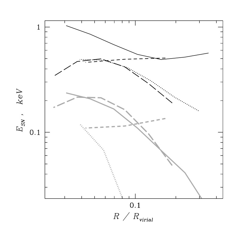
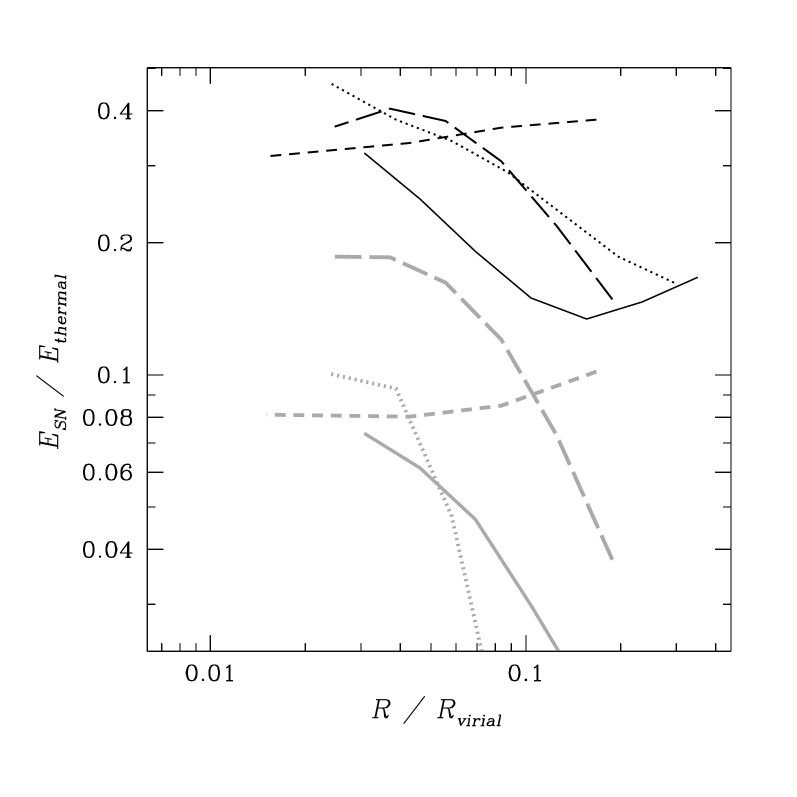
Figure 34: Thermal energy associated with SNe (left panel) and relative to the thermal energy of the gas (right panel). Line coding is similar to Fig.30. Contributions of SN Ia are shown in grey.

4.4 Supernovae, energy balance and gas fraction

On the assumption that the metals measured in our systems are direct products of SNe activity we can calculate the total energy supplied by SNe and estimate their role in the energy balance of these systems.

In Fig.34 we present a comparison of the energy released by SNe, $E_{sn}$, versus the thermal energy of the gas, $E_{th}$. Units chosen are keV, and the SNe values were obtained by finding the number of SN Ia and SN II needed to reproduce the measured Fe and Si masses (which are in turn derived from local metallicities) and assuming that each SN releases $10^{51}$ ergs which is completely mixed with the gas.

Whilst SN Ia and SN II contribute comparable amounts of Fe from our analysis, the much larger iron yield of SN Ia (0.744$M_{\odot}$ of released Fe, compared to 0.121$M_{\odot}$ in SN II) implies that the total number of SNe, and hence the total energy release, is dominated by SN II. This can be clearly seen in the figure.

A number of uncertainties affect our estimates of energy injection. Firstly we have assumed that all the SN II contribution is injected directly into the IGM by supernovae. As discussed above, any stellar wind material which manages to escape from galaxies will appear primarily within our ‘SN II’ component, yet its injection is likely to be a less energetic process. This, together with the fact that some of the supernova energy will be radiated rather than lost as kinetic energy, means that our calculated energy injection may be regarded as an upper limit. We also neglect the energy expended in releasing the gas from galaxy’s potential well. On the other hand, the gas is released into the system with an additional energy due to the velocity dispersion of galaxies, which more than compensates for this loss. The sub-solar abundances found in our systems argue in favour of strong dilution of the galactic wind by primordial gas, which will effectively thermalise the kinetic energy of galaxy ejecta.

In addition, the uncertainties in SN II yields discussed above leads to corresponding uncertainties in energy considerations. Moreover, as is shown by the calculations of W95, SN II from low metallicity progenitors provide a similar Si/Fe ratio, but a much smaller mass of the released metals, thus introducing a scaling factor to the SN II associated energy. In the present calculation we adopt the metal yields of the T95 model, which assume solar metallicity progenitors. If a lower metallicity population were assumed, the inferred SN II energy would increase.

The main points to note from Fig.34 are the low contribution of SN Ia to the energy budget of the IGM, the significant contribution (around 20–40 per cent) of SN II, and the fact that the SNe-released energy is more important in the poorer systems. Since the effect of significant wind injection is primarily to reduce the gas density, by raising its entropy (Cavaliere, Menci & Tozzi 1997; Ponman, Cannon & Navarro 1999), these results support the picture whereby the steepening of the $L:T$ relation at low temperatures is a fossil remnant of the activity generated by active star formation in galaxies (Ponman et al. 1996).

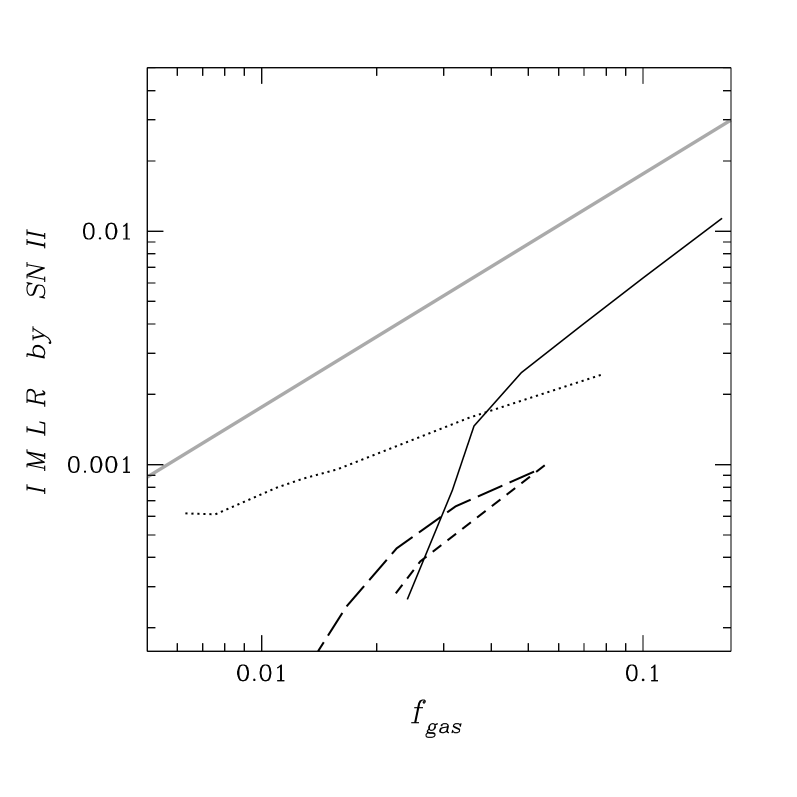
Figure 36: Gas fraction vs IMLR contributed by SN II. Line coding is similar to Fig.30. The expected behaviour of systems with complete mixing of the SN ejecta with primordial gas is shown by a thick grey line.

Considering the energy release by SN II, we should take into account the effects of possible metal loss from the system, which is suggested by the low IMLR in the three groups compared to clusters. If gas is lost pro-rata, along with the metals, then the ratio of SN energy to thermal energy (which is our main concern here) will be unaffected. However, it is possible that hot enriched material might escape preferentially – for example if the hot SN-driven wind is not completely mixed with the primordial gas and escapes without pushing all the metal-poor gas away or some of the galaxies expelled elements before collapsing into the primordial gas of groups or clusters, thus bringing light but not metals. We can explore the possibility of gas loss by comparing the observed IMLR and gas fractions ($f_{\rm gas}$) with those of rich clusters, in which it is reasonable to suppose that gas loss is minimal. In Fig.36, we plot the relationship between IMLR and the cumulative gas fraction $f_{\rm gas}$ (calculated as $M_{gas}(<r)/M_{total}(<r)$) within our observed systems. Taking representative values within the main bodies of clusters to be an IMLR of 0.02 (Arnaud et al. 1992) and gas fraction value of 0.17 (e.g.  Evrard 1997), we draw a line IMLR${}_{\rm SN~{}II}\propto f_{\rm gas}$ passing through this point. Loss of well mixed gas would move a system down this line, whereas preferential loss of metal rich gas, or accretion of metal-poor gas, would cause it to fall below the line.

It appears, by investigating the Fig.36, that distributions of the elements and the gas are correlated and so the changes in gas mass fraction within one system could be explained by energy release in SN II explosions. Although, systems demonstrate different amount of metals at a given gas mass fraction, the difference between the groups is more then the difference between the cluster and the groups. It might be that the age of the group formation is different among the systems studied here, with HCG51 and NGC5044 being the youngest. We note that the behaviour of HCG62 and NGC5044 at large radii, where the IGM gains more gas than metals, is consistent with the idea that primordial gas may have accreted onto the system (cf Brighenti & Mathews, 1998).

5 Conclusions – supernovae and hierarchical clustering

We have derived temperature and abundance profiles for a set of groups of galaxies, NGC5044, HCG51 and HCG62, and compared the results with a poor cluster AWM7. A decrease in abundances with radius is detected in all but HCG51, which we suggest may have undergone recent disruption of its IGM, probably due to a major merger. In AWM7 we find also a flattening of the abundance gradients of Ne, Si, S and Fe outside a radius of 200 kpc, correlated with a change in the abundance ratio favouring a high Si/Fe ratio in the outer parts of the cluster.

We have compared the derived element abundances with the predictions of several theoretical models and Si and Fe abundance measurements as most consistently modeled in SN Ia – SN II reference frame. Employing T95 model for the average stellar SN II yields and TNH93 model for SN Ia yields, we use the spatially resolved profiles of iron and $\alpha$-elements to decompose the iron profile into separate contributions from SN Ia and SN II. Having explored their behaviour, derived the IMLR, and compared the expected SN energy with the thermal energy of the gas, we derive the following conclusions:

• SN Ia and SN II have both made a significant contribution to the enrichment of the intergalactic medium. The contribution from SN Ia reduces the need to invoke a flat IMF in order to explain the total mass of heavy elements found in the IGM (Wyse 1997).

• SN II products are distributed widely within the IGM, which probably indicates that they were released at early times in cluster formation via energetic galaxy winds. Clusters have retained the SN II products more effectively than groups at all radii from 0.05 to at least 0.4 of $R_{virial}$.

• The distribution of iron abundance attributed to SN Ia is centrally peaked, with a core radius comparable to the optical radius of the system. This indicates the dominance of gas release mechanisms which are strongly density-dependent, such as gas ablation, dark halo stripping and galaxy-galaxy interactions. Significant quantities of SN Ia products also appear to have been lost from the shallower potential wells of groups, suggesting the importance of energetic injection at late times, presumably through SN Ia-driven winds.

• The central rise in the $\alpha$-element abundances seen in AWM7 is probably a product of mass loss from the cD galaxy.

• While the SN Ia energy is small compared to the thermal energy of the gas, the SNe II contribution could amount to $\sim 20-40$ per cent, which would have a substantial effect on the structure of the intracluster medium in low mass systems.

This paper has been produced using the Royal Astronomical Society/Blackwell Science LaTEX style file.

References

- 1
- 2 Anders E. and Grevesse N. 1989, Geochimica et Cosmochimica Acta, 53, 197
- 3 Arimoto N., Matsushita K., Ishimaru Y., Ohashi T., Renzini A 1997, ApJ, 477, 128
- 4 Arnaud M. et al. 1992, A&A, 254, 49
- 5 Beers T.C., Geller M.J., Huchra J.P., Latham D.W., Davis R.J. 1984, ApJ, 283, 33
- 6 Burke B.E., Mountain R.W., Harrison D.C., Bautz M.W., Doty J.P., Ricker G.R. and Daniels P.J. 1991, IEEE Trans., EED-38, 1069
- 7 Blumenthal G.R., Faber S.M., Primack J.R., Rees M.J. 1984, Nat, 517, 311
- 8 Brighenti F., Mathews W. G. 1998, ApJ, 495, 239
- 9 Carlberg R.G. 1984, ApJ, 286, 408
- 10 Cavaliere A., Menci N. and Tozzi P. 1997, ApJ, 484, L21
- 11 Churazov E., Gilfanov M., Forman W., Jones C. 1996, ApJ, 471, 673
- 12 David L., Jones C., Forman W. and Daines S. 1994, ApJ, 428, 544
- 13 De Carvalho R.R., Ribeiro A.L.B., Capelato H.V. and Zepf S.E. 1997, ApJS, 110, 1
- 14 Eyles et al. 1991, ApJ, 376, 23
- 15 Ezawa H. et al. 1997, ApJ, 490, L33
- 16 Ferguson H.C. and Sandage A. 1990, AJ, 100, 1
- 17 Finoguenov A., Jones C., Forman W. and David L. 1999, ApJ, April issue, (also astro-ph/9810107).
- 18 Fukazawa et al. 1996, PASJ, 48, 395
- 19 Fukazawa 1997, Ph.D. Thesis, Univ. of Tokyo
- 20 Fukazawa Y. et al. 1998, PASJ, 50, 187
- 21 Gibson B.K., Loewenstein M. and Mushotzky R.F. 1997, MNRAS, 290, 623
- 22 Hickson P. 1982, ApJ, 255, 382
- 23 Hickson P., Mendes de Oliveira C., Huchra J.P., Palumbo G.G.C. 1992, ApJ, 399, 353
- 24 Hickson P. 1997, Preprint Astro-ph No. 9710289
- 25 Jones C. and Forman W. 1984, ApJ, 276, 38
- 26 Lampton M., Margon B. & Bowyer S. 1976, ApJ, 208, 177
- 27 Liedahl D.A., Osterheld A.L. and Goldstein W.H. 1995, ApJ, 438, L115
- 28 Loewenstein M. and Mushotzky R.F. 1996, ApJ, 466, 695
- 29 Markevitch M. & Vikhlinin A. 1997, ApJ, 474, 84
- 30 Mathews W.G. 1989, AJ, 97, 42
- 31 Matsushita K., Makishima K., Ikebe Ya., Rokutanda E., Yamasaki N., Ohashi T., 1998, ApJ (Letters), 499, 13
- 32 Matteuci F. & Gibson B.K. 1995, A&A, 304, 11
- 33 Mewe R., Gronenschild E.H.B.M. and Oord G.H.J. 1985, A&AS, 62, 197
- 34 Mewe R. & Kaastra J. 1995, Internal SRON-Leiden report
- 35 Mulchaey J. S., Davis D.S., Mushotzky R.F., Burstein D. 1996, ApJ, 456, 80
- 36 Mushotzky R.F., Loewenstein M., Arnaud K.A., Tamura T., Fukazawa Y., Matsushita K., Kikuchi K. and Hatsukade I. 1996, ApJ, 466, 686
- 37 Neumann D.M. & Boehringer H. 1995, A&A, 301, 865
- 38 Ponman T.J. and Bertram D. 1993, Nat, 363, 51
- 39 Ponman T.J. Bourner P.D.J., Ebeling H. and Boehringer H. 1996, MNRAS, 283, 690
- 40 Ponman T.J., Cannon D.B. and Navarro J.F. 1999, Nat, , in press
- 41 Press W.H., Teukolsky S.A., Vetterling W.T., Flannery B.P. 1992, Numerical recipes in FORTRAN
- 42 Raymond J. and Smith B. 1977, ApJS, 35, 419
- 43 Renzini et al. 1993, ApJ, 419, 52
- 44 Schweizer F. and Seitzer P. 1992, AJ, 104, 1039
- 45 Snowden S. et al. 1994, ApJ, 424, 714
- 46 Takahashi et al. 1995 ASCA Newsletter, no.3 (NASA/GSFC)
- 47 Tamura T., Day C.S., Fukazawa Y., Hatsukade I., Ikebe Y. et al. 1996, PASJ, 48, 671
- 48 Tanaka Y., Inoue H. and Holt S.S. 1984, PASJ, 46, L37
- 49 Thielemann, F.-K., Nomoto, K. & Hashimoto, M. 1993 Origin and Evolution of the Elements. (ed. N.Prantzos, E.Vangioni-Flam & M. Cassé). Cambridge Univ. Press, 297
- 50 Thielemann, F.-K., Nomoto, K. & Hashimoto 1996, ApJ, 460, 408
- 51 Truemper J. 1983, Adv. Space Res., 2, 241
- 52 Tsujimoto T., Nomoto K., Yoshii Y., Hashimoto M., Yanagida S. and Thielemann F.-K. 1995, MNRAS, 277, 945
- 53 Worthey G., Faber S.M. and Gonzalez J.J. 1992, ApJ, 398, 69
- 54 Woosley S.E. and Weaver T.A. 1995, ApJS, 101, 181
- 55 Wyse R.F.G. 1997, ApJ, 490, L69
- 56 Yoshii Y., Tsujimoto T., Nomoto K. 1996, ApJ, 462, 266