Power Spectrum Correlations Induced by Non-Linear Clustering

Abstract

Gravitational clustering is an intrinsically non-linear process that generates significant non-Gaussian signatures in the density field. We consider how these affect power spectrum determinations from galaxy and weak-lensing surveys. Non-Gaussian effects not only increase the individual error bars compared to the Gaussian case but, most importantly, lead to non-trivial cross-correlations between different band-powers, correlating small-scale band-powers both among themselves and with those at large scales. We calculate the power-spectrum covariance matrix in non-linear perturbation theory (weakly non-linear regime), in the hierarchical model (strongly non-linear regime), and from numerical simulations in real and redshift space. In particular, we show that the hierarchical ansatz cannot be strictly valid for the configurations of the trispectrum involved in the calculation of the power-spectrum covariance matrix.

We discuss the impact of these results on parameter estimation from power-spectrum measurements and their dependence on the size of the survey and the choice of band-powers. We show that the non-Gaussian terms in the covariance matrix become dominant for scales smaller than the non-linear scale $k_{nl}\sim 0.2$ h/Mpc, depending somewhat on power normalization. Furthermore, we find that cross-correlations mostly deteriorate the determination of the amplitude of a rescaled power spectrum, whereas its shape is less affected. In weak lensing surveys the projection tends to reduce the importance of non-Gaussian effects. Even so, for background galaxies at redshift $z\sim 1$, the non-Gaussian contribution rises significantly around $l\sim 1000$, and could become comparable to the Gaussian terms depending upon the power spectrum normalization and cosmology. The projection has another interesting effect: the ratio between non-Gaussian and Gaussian contributions saturates and can even decrease at small enough angular scales if the power spectrum of the 3D field falls faster than $k^{-2}$.

CITA-98-62, FERMILAB-Pub-99/003-A

1 Introduction

Discussions in the literature on the measurement of the power spectrum $P(k)$ (e.g. Feldman et al. (1994)), and the estimation of cosmological parameters from it (e.g. Tegmark 1997b ; Eisenstein et al. (1998); Hu & Tegmark (1998)), have largely focused on the case of Gaussian random data. While this is a reasonable assumption in the case of the cosmic microwave background for Gaussian initial conditions (e.g. Tegmark (1997); Bond et al. (1998); Seljak (1998)), it is probably not a good approximation for galaxy and weak-lensing surveys except on sufficiently large scales (e.g. Feldman et al. (1994); Vogeley & Szalay (1996); Hamilton (1997); Colombi et al. (1998); Seljak 1998b ; Tegmark et al. (1998); Dodelson et al. (1997)). This is because of the non-Gaussianity inevitably induced by gravitational clustering, which leads to increased error bars in individual band-power estimates and introduces correlations between them. In this paper, we quantify the size of these effects and the scales at which they become important.

Understanding the statistical properties of power-spectrum estimators beyond the Gaussian approximation requires at least a calculation of the power-spectrum covariance matrix, which involves the four-point function of the density field in Fourier space, the trispectrum. In order to do this, we use both analytic and numerical techniques. At weakly non-linear scales, non-linear perturbation theory (PT) can be used to understand quantitatively how the non-Gaussian effects are generated through mode-coupling. We provide a calculation of the relevant configurations of the trispectrum, and use them to obtain the covariance matrix of band-powers.

Non-Gaussian effects are most significant at non-linear scales, where PT breaks down. To investigate this regime, we resort to numerical simulations, which we use to evaluate the power-spectrum covariance matrix by measuring the power spectrum in several realizations. At small scales, where virialization is reached, stable clustering suggests a simple behavior of higher-order correlation functions, known as the hierarchical ansatz. We use these arguments to understand the power-spectrum covariance matrix in the non-linear regime, which in turn allows us to extend in a simple way our results to the projected density field.

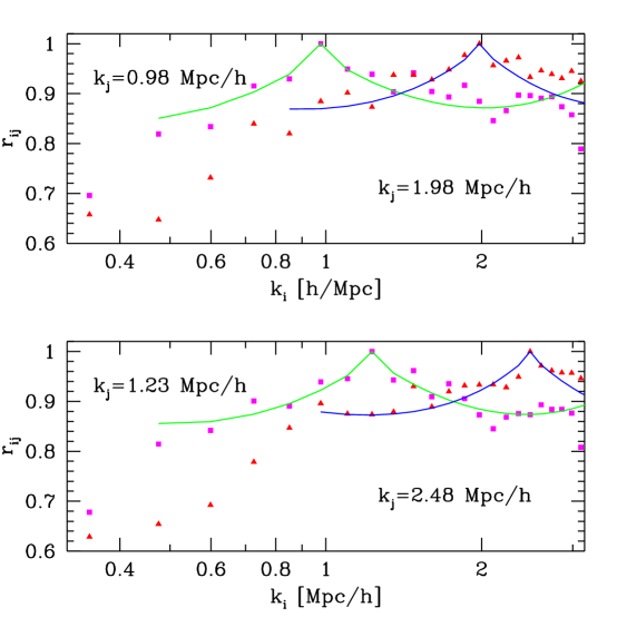
Figure 9: Correlation coefficients $r_{ij}$ in the non-linear regime predicted by HEPT (solid lines) for $R_{a}\approx R_{b}$ compared with those from numerical simulations (symbols). The width of shells in $k$-space is $\delta k=4\pi/100$ h/Mpc.

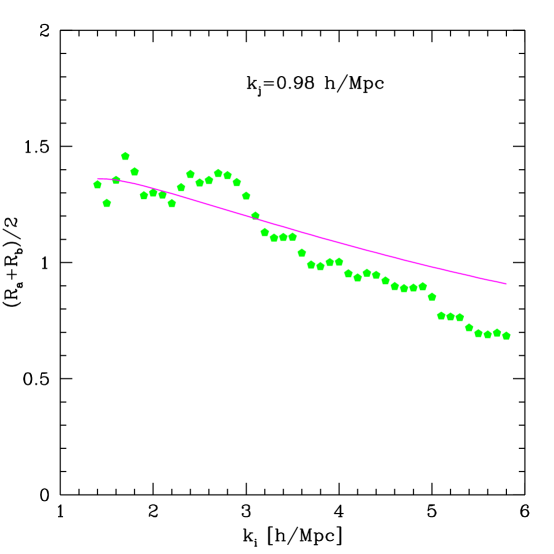
Figure 10: Estimate of $(R_{a}+R_{b})/2$ from the measured power-spectrum covariance matrix, for $k_{j}=0.98$ h/Mpc, as a function of $k_{i}$, using equations (17-18). The solid lines show the expected $(R_{a}+R_{b})/2$ value assuming that the configuration dependence in the non-linear regime is the same as that given by PT.

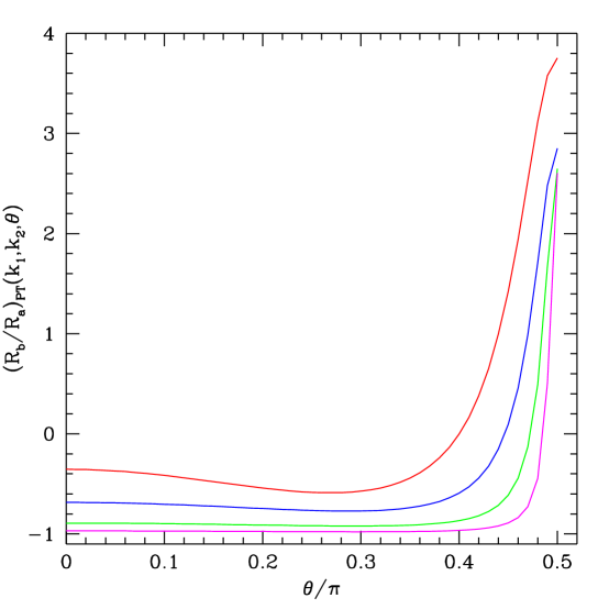
Figure 11: The ratio $R_{b}/R_{a}$ given by PT as a function of configuration angle $\theta$ between ${{\hbox{\BF k}}}_{1}$ and ${{\hbox{\BF k}}}_{2}$ for different scales. From top to bottom, $(k_{1},k_{2})=(1,2)$ h/Mpc, $(1,4)$ h/Mpc, $(1,8)$ h/Mpc, and $(1,16)$ h/Mpc. Note how the relation $R_{a}=-R_{b}$ eventually holds for most configurations as the shells become very distant.

The outline of the paper is as follows. In §2, we introduce the notations and basic expressions for the covariance matrix of the 3D (three-dimensional) power-spectrum estimates. Here, as in the rest of the paper, we focus on the sample-variance dominated regime. In other words, shot-noise is ignored - the emphasis here is on the effect of non-Gaussianity induced by gravitational clustering. Shot-noise will be included in a separate treatment. We present estimates of the power-spectrum covariance matrix using PT, numerical simulations and the hierarchical model in §3.1, 3.2 and 3.3, respectively. In particular, we show in the latter that the hierarchical ansatz does not provide a good description of the covariance matrix in the non-linear regime, because there are always contributions coming from large scales (§3.3.1). Instead, we find that the covariance matrix behaves as a “generalized” hierarchical model, with configuration dependence that resembles that in PT (Figs. 9-11). On the other hand, for trispectrum configurations fully in the non-linear regime, we verify the validity of the hierarchical ansatz and provide some new results concerning the importance of different contributions (Fig.8).

The impact of non-Gaussianity on parameter determination is illustrated in §4 with a simple example, in which the amplitude of the power spectrum is the only parameter of interest. We discuss the impact on the determination of the power spectrum shape as well. In all of the discussions above, it is implicitly assumed one can measure the mass power spectrum directly. This is of course complicated by biasing in the case of galaxy surveys. In fact, as we shall see, on scales where non-Gaussianity is non-negligible, galaxy-biasing is also likely to be non-trivial. Weak gravitational lensing (e.g. Blandford et al. (1991); Miralda-Escudé (1991); Kaiser (1992); Bernardeau et al. (1997); Jain & Seljak (1997); Kaiser (1998); Seljak 1998b ; van Waerbeke et al. (1999)) promises to be a bias-free way to measure the mass power spectrum, but as we will show in §5, weak-lensing surveys in the near future will likely cover small angular scales and thus receive significant contributions from non-linear fluctuations to the expected signals. In §5, we derive the appropriate expression for the covariance matrix of the projected mass power spectrum, and show that the projection reduces the non-Gaussian effects of the matter distribution, but non-negligible residuals remain. In fact, for low matter density models where the cluster normalization implies larger rms density fluctuations, the non-Gaussian contribution to the covariance can dominate over the Gaussian value (van Waerbeke et al. (1999)). Finally, we conclude in §6 with a discussion.

2 Definitions

We shall be interested in the Fourier modes of the overdensity $\delta(\hbox{\boldmath{$x$}})$ given by,

$$\delta(\hbox{\boldmath{$k$}})=\int\frac{d^{3}{{\hbox{\BF x}}}}{(2\pi)^{3}}\ e^{-i\hbox{\boldmath{$k$}}\cdot\hbox{\boldmath{$x$}}}\ \delta(\hbox{\boldmath{$x$}})\,.$$ (1)

Their statistical properties are described by the various connected moments,

$$\langle\delta({\hbox{\BF k}}_{1})\rangle_{c} = 0$$

$$\langle\delta({\hbox{\BF k}}_{1})\delta({\hbox{\BF k}}_{2})\rangle_{c} = \delta_{\rm D}({\hbox{\BF k}}_{12})\ P({\hbox{\BF k}}_{1})$$

$$\langle\delta({\hbox{\BF k}}_{1})\delta({\hbox{\BF k}}_{2})\delta({\hbox{\BF k}}_{3})\rangle_{c} = \delta_{\rm D}({\hbox{\BF k}}_{123})\ B({\hbox{\BF k}}_{1},{\hbox{\BF k}}_{2},{\hbox{\BF k}}_{3})$$

$$\langle\delta({\hbox{\BF k}}_{1})\delta({\hbox{\BF k}}_{2})\delta({\hbox{\BF k}}_{3})\delta({\hbox{\BF k}}_{4})\rangle_{c} = \delta_{\rm D}({\hbox{\BF k}}_{1234})\ T({\hbox{\BF k}}_{1},{\hbox{\BF k}}_{2},{\hbox{\BF k}}_{3},{\hbox{\BF k}}_{4})$$

$$\langle\delta({\hbox{\BF k}}_{1})\delta({\hbox{\BF k}}_{2})\cdots\delta({\hbox{\BF k}}_{n})\rangle_{c} = \delta_{\rm D}({\hbox{\BF k}}_{12\cdots n})\ T_{n}({\hbox{\BF k}}_{1},{\hbox{\BF k}}_{2},\cdots,{\hbox{\BF k}}_{n}),$$ (2)

where ${\hbox{\BF k}}_{i...j}\equiv{\hbox{\BF k}}_{i}+\cdots+{\hbox{\BF k}}_{j}$, with $\delta_{\rm D}(x)$ denoting the Dirac delta distribution. In equation (2), $P(k)$, $B({\hbox{\BF k}}_{1},{\hbox{\BF k}}_{2},{\hbox{\BF k}}_{3})$ and $T({\hbox{\BF k}}_{1},{\hbox{\BF k}}_{2},{\hbox{\BF k}}_{3},{\hbox{\BF k}}_{4})$ denote the power spectrum, bispectrum and trispectrum, respectively. For the purpose of this paper we will need up to the fourth connected moment.

Let’s suppose we are given a survey with volume $V$, from which $\delta(\hbox{\boldmath{$k$}})$ can be constructed. We divide the Fourier space into shells (or bands) of width $\delta k$ centered on $k_{i}=i\times\delta k,i=1,2,...$, and then average the variance of the k modes within each shell to obtain the following estimate of the power spectrum,

$${\hat{P}}(k_{i}) = V_{f}\int_{k_{i}}{d^{3}{\hbox{\BF k}}\over V_{s}(k_{i})}\ \delta({\hbox{\BF k}})\delta(-{\hbox{\BF k}})$$ (3)

where the integration extends over modes within the shell centered at $k_{i}$, $V_{s}(k_{i})=4\pi k_{i}^{2}\delta k$ is the volume of the shell, and $V_{f}$ is the volume of the fundamental cell in $k$ space, $V_{f}=(2\pi)^{3}/V$. For the rest of this paper, we will also use $P_{i}$ interchangeably with $P(k_{i})$ wherever confusion will not arise. It is straightforward to calculate the covariance matrix of the power spectrum estimators. Combining equations (2) and (3), we get

$${C}_{ij} \equiv \langle{\hat{P}}(k_{i}){\hat{P}}(k_{j})\rangle-\langle{\hat{P}}(k_{i})\rangle\langle{\hat{P}}(k_{j})\rangle=V_{f}\ [{2P_{i}^{2}\over V_{s}(k_{i})}\delta_{ij}+{\bar{T}}(k_{i},k_{j})]$$ (4)

where $\delta_{ij}$ is the Kronecker delta and $\bar{T}$ is the bin-averaged trispectrum

$${\bar{T}}(k_{i},k_{j}) = \int_{k_{i}}{d^{3}{{\hbox{\BF k}}_{1}}\over V_{s}(k_{i})}\ \int_{k_{j}}{d^{3}{{\hbox{\BF k}}_{2}}\over V_{s}(k_{j})}\ T({\hbox{\BF k}}_{1},-{\hbox{\BF k}}_{1},{\hbox{\BF k}}_{2},-{\hbox{\BF k}}_{2}).$$ (5)

The first term in equation (4) is the Gaussian contribution. In the Gaussian limit, each Fourier mode is an independent Gaussian random variable. The power estimates of different bands are therefore uncorrelated, and the covariance is simply given by $2/N_{k_{i}}$ where $N_{k_{i}}$ is the number of independent Gaussian variables, i.e. $N_{k_{i}}=V_{s}(k_{i})/V_{f}$. The second term in equation (4) arises because of non-Gaussianity, which generally introduces correlations between different Fourier modes, and hence it is not diagonal in general.

Both terms in the covariance matrix in equation (4) are proportional to $V_{f}$, or inversely proportional to $V$, the volume of the survey. But the Gaussian and non-Gaussian contributions scale in a different way with $V_{s}$: while the Gaussian contribution decreases with the size of the shell, the non-Gaussian term remains constant. Therefore, when the covariance matrix is dominated by the non-Gaussian contribution the only way to reduce the variance of the power spectrum is to increase the volume of the survey instead of averaging over more Fourier modes.

It is worth emphasizing here that we have ignored the effect of the survey window in the above expressions. We have implicitly assumed the modes of interest have wavelengths much smaller than the size of the survey, which is likely to be a good approximation as we are interested in the non-Gaussianity induced by gravity on small scales (how small is small is a question we will address). Note also that while $\delta({\hbox{\BF k}})$ is not restricted to be the mass overdensity in the above expressions, we will assume so in the rest of the paper. Galaxy surveys of course only probe directly the galaxy rather than the mass overdensity. For the most part, we ignore galaxy biasing in this paper. We will come back to this issue in the final section.

3 Covariance Matrix of the Band-Power Estimates in 3D

In structure formation scenarios where the initial conditions are Gaussian, the power-spectrum covariance matrix is expected to be diagonal on sufficiently large scales, with amplitude given by the first term in equation (4). Gravitational clustering, however, inevitably generates a non-vanishing trispectrum through non-linear mode-coupling. It is thus expected that at small enough scales, the non-Gaussian contribution to the power-spectrum covariance matrix (second term in equation [4]) will dominate over the Gaussian term.

To demonstrate this, we use non-linear perturbation theory (PT) to calculate at what scales significant non-Gaussian contributions first appear. We then use numerical simulations to measure their effects on smaller, non-linear scales, where PT breaks down. In the highly non-linear regime we study the validity of the hierarchical model for the trispectrum, and calibrate it using N-body simulations and Hyperextended PT (Scoccimarro & Frieman (1998)).

3.1 The Power-Spectrum Covariance Matrix in PT

In tree-level (leading-order) PT, the trispectrum is given by (see e.g. Fry (1984)):

$$T({\hbox{\BF k}}_{1},{\hbox{\BF k}}_{2},{\hbox{\BF k}}_{3},{\hbox{\BF k}}_{4}) = 4[F_{2}({\hbox{\BF k}}_{12},-{\hbox{\BF k}}_{1})\ F_{2}({\hbox{\BF k}}_{12},{\hbox{\BF k}}_{3})\ P_{1}P_{12}P_{3}+{\rm cyc.}]+6[F_{3}({\hbox{\BF k}}_{1},{\hbox{\BF k}}_{2},{\hbox{\BF k}}_{3})\ P_{1}P_{2}P_{3}+{\rm cyc.}],$$ (6)

where $P_{i}\equiv P(k_{i})$, with ${\hbox{\BF k}}_{12}={\hbox{\BF k}}_{1}+{\hbox{\BF k}}_{2}$ as defined before, “cyc.” denotes cyclic permutation of the arguments (12 terms in total in the first contribution, and 4 terms in the second contribution), and the kernels $F_{n}$ are obtained from solving the equations of motion of gravitational instability to $n^{\rm th}$ order in PT (Goroff et al. (1986)). Equation (5) tells us that only a particular class of trispectrum configurations (parallelogram) contributes to the non-Gaussian covariance of the band-power estimates. Substituting the above expression into equation (5), we have

$${\bar{T}}(k_{i},k_{j}) = \int_{k_{i}}{d^{3}{{\hbox{\BF k}}_{1}}\over V_{s}(k_{i})}\ \int_{k_{j}}{d^{3}{{\hbox{\BF k}}_{2}}\over V_{s}(k_{j})}\ \Big{[}12F_{3}({\hbox{\BF k}}_{1},-{\hbox{\BF k}}_{1},{\hbox{\BF k}}_{2})P_{1}^{2}P_{2}+8F_{2}^{2}({\hbox{\BF k}}_{1}-{\hbox{\BF k}}_{2},{\hbox{\BF k}}_{2})P(|{\hbox{\BF k}}_{1}-{\hbox{\BF k}}_{2}|)P_{2}^{2}$$ (7)

$$+ 16F_{2}({\hbox{\BF k}}_{1}-{\hbox{\BF k}}_{2},{\hbox{\BF k}}_{2})F_{2}({\hbox{\BF k}}_{2}-{\hbox{\BF k}}_{1},{\hbox{\BF k}}_{1})P_{1}P_{2}P(|{\hbox{\BF k}}_{1}-{\hbox{\BF k}}_{2}|)+({\hbox{\BF k}}_{1}\leftrightarrow{\hbox{\BF k}}_{2})\Big{]}$$

Using the facts that $[F_{2}({\hbox{\BF k}}_{1}-{\hbox{\BF k}}_{2},{\hbox{\BF k}}_{2})]_{k_{1}=k_{2}}=(3+10x)/28$, where $x\equiv{\hat{k}}_{1}\cdot{\hat{k}}_{2}$, and that the angular average $\mathop{\langle}F_{3}({\hbox{\BF k}}_{1},-{\hbox{\BF k}}_{1},{\hbox{\BF k}}_{2})\mathop{\rangle}_{k_{1}=k_{2}}=-11/378$, plus the approximate angular-averaged result

$$\int_{-1}^{1}\frac{dx}{2}\ \Big{(}\frac{3+10x}{28}\Big{)}^{2}P(\sqrt{2(1-x)}k)\approx\frac{30}{784}\ P(k),$$ (8)

a simple approximate expression for the diagonal components of the band-averaged trispectrum follows

$${\bar{T}}(k_{i},k_{i})\approx\frac{232}{441}\ P_{i}^{3}\,,$$ (9)

where we have further assumed that the power spectrum is approximately constant within the shell. Note that the non-Gaussian terms scale as the power spectrum cubed, therefore, to be consistent within PT, one-loop corrections to the power spectrum in the diagonal Gaussian term must be included.

Figure 1 shows the diagonal elements of the covariance matrix, divided by the Gaussian contribution, calculated using perturbation theory for a survey with $V=1{\rm(Gpc/h)^{3}}$ . The cosmological model we assume throughout the paper is standard cold dark matter (SCDM) with $\sigma_{8}=0.60$. The increase in the diagonal variance relative to the Gaussian variance is very small, less than $1\%$ for $k<0.2$, which in part reflects the small bin-size considered, $\delta k=2\pi$ h/Gpc. The non-linear scale, where $4\pi k^{3}P(k)=1$, is given by $k_{nl}=0.33$. It is important to emphasize that figure 1 depends on the binning adopted. In other words, the relative importance of the Gaussian and non-Gaussian variances for each band is dependent upon the size of the band.

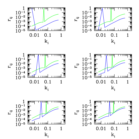
Figure 2: Correlation coefficients $r_{ij}\equiv C_{ij}/[C_{ii}C_{jj}]^{1/2}$ as a function of $k_{i}$ for different fixed $k_{j}$ obtained using PT for a 1 Gpc/h box, and the SCDM model. The $k$ shells are the same as in figure 1. The values of $k_{j}$ can be inferred from the place where $r_{ij}=1$. In each panel we plot the results for two different values of $k_{j}$.

In figure 2 we show some of the off-diagonal elements, in terms of the cross-correlation coefficient $r_{ij}\equiv C_{ij}/\sqrt{C_{ii}C_{jj}}$. Each curve in figure 2 corresponds to $r_{ij}$ as a function of $k_{i}$ for a fixed $k_{j}$. The corresponding $k_{j}$ can be inferred from where $r_{jj}=1$. By definition each $r_{ij}$ is independent of the volume of the survey but it does depend on the $k$-space binning. In this case, the binning has been chosen to be constant with the smallest possible value, $\delta k=2\pi$ h/Gpc, which maximizes the Gaussian contribution. The correlation coefficients $r_{ij}$, for $i\neq j$, are therefore quite small. A logarithmic binning would change the appearance of the figures. It is important to emphasize that although the correlation coefficients are small, there are also many of them. In fact because the size of the correlation coefficients depends on the choice of band-powers, they do not have a direct physical meaning. In the limit we are considering in this section, where the diagonal terms of the covariance are dominated by the Gaussian contributions we have in fact $r_{ij}\propto\delta k$. In §4 we will address the importance of the non-Gaussian terms in a way independent of the binning procedure.

In order to understand the origin of power spectrum cross-correlations, let us consider the integrand in equation (7), $T({\hbox{\BF k}}_{1},-{\hbox{\BF k}}_{1},{\hbox{\BF k}}_{2},-{\hbox{\BF k}}_{2})\equiv T_{4}({\hbox{\BF k}}_{1},{\hbox{\BF k}}_{2})$, and normalize it according to

$$\beta_{12}({\hbox{\BF k}}_{1},{\hbox{\BF k}}_{2})\equiv T_{4}({\hbox{\BF k}}_{1},{\hbox{\BF k}}_{2})\ \sqrt{\frac{1}{2P_{1}^{2}}\frac{1}{2P_{2}^{2}}\frac{V_{s}(k_{1})V_{s}(k_{2})}{\Delta(k_{1})\Delta(k_{2})}}=\frac{1}{2}\frac{T_{4}({\hbox{\BF k}}_{1},{\hbox{\BF k}}_{2})}{(P_{1}P_{2})^{3/2}}\sqrt{\frac{\delta k_{1}\delta k_{2}}{k_{1}k_{2}}},$$ (10)

where $\Delta(k)\equiv 4\pi k^{3}P(k)$. We then obtain

$$C_{ij}=V_{f}\ \frac{2P_{i}P_{j}}{\sqrt{V_{s}(k_{i})V_{s}(k_{j})}}\ [\delta_{ij}+{\bar{\beta}}_{ij}\sqrt{\Delta(k_{i})\Delta(k_{j})}],$$ (11)

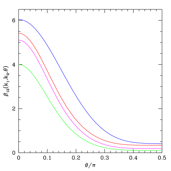
Figure 3: The coefficient $\beta_{12}(k_{1},k_{2},\theta)$ [equation (10)] as a function of $\theta$ for different scales. From top to bottom, $(k_{1},k_{2})=(0.1,0.4)$ h/Mpc, $(0.1,0.2)$ h/Mpc, $(0.2,0.4)$ h/Mpc, and $(0.4,0.8)$ h/Mpc.

with ${\bar{\beta}}_{ij}$ the bin-averaged version of $\beta_{12}$. Figure 3 shows the coefficient $\beta_{12}$ as a function of configuration angle $\theta$ between ${\hbox{\BF k}}_{1}$ and ${\hbox{\BF k}}_{2}$ for different scales, assuming constant bin size as a function of scale $\delta k_{1}=\delta k_{2}=2\pi/100$ h/Mpc. This figure illustrates how modes get correlated, the maximum amplitude of correlation results for co-linear configurations ($\theta=0$), and the least amount of correlation corresponds to perpendicular modes ($\theta=\pi/2$). This is exactly what is expected for structures formed by gravitational instability (Scoccimarro (1997); Scoccimarro et al. (1998)). It would be interesting to take advantage of this pattern of correlations to build a power spectrum estimator that minimizes the amount of cross-correlations.

3.2 The Power-Spectrum Covariance Matrix in Numerical Simulations

We measured the power spectrum from 20 different PM simulations of the SCDM model with $\sigma_{8}=0.60$ and a box-size of 100 Mpc/h with $128^{3}$ particles and a $256^{3}$ force grid. Figure 4a shows the diagonal elements of the covariance matrix normalized by the Gaussian variance, obtained by computing the power spectra in the 20 PM simulations and performing the ensemble average. The dashed line at weakly non-linear scales shows the predictions of PT, equation (9). As predicted by PT, the increase in the diagonal covariance due to non-Gaussian effects is quite small, even at the non-linear scale $\Delta(k_{nl})=1$ (shown in the plot as a vertical line). We see that the diagonal terms of the covariance matrix increase rapidly relative to the the Gaussian contributions, once the non-linear regime is reached.

In the bottom panel we show the same diagonal components but normalized by $P$, which yields the fractional errors in the power spectrum estimates: $\sigma_{P}/P$. The fractional error decreases with increasing $k_{i}$ as $k_{i}^{-2}$ for linear scales but does so much more slowly once we enter the non-linear regime. It should be stressed that the quantities shown depend both on the assumed binning in $k$-space and on the volume of the simulation box. Unless otherwise stated, all our measurements in numerical simulations are done using a constant bin size, $\delta k=2\pi/100$ h/Mpc, the fundamental mode of the simulation box. On the other hand, at sufficiently non-linear scales the covariance matrix becomes independent of the binning (but it is still inversely proportional to the simulation volume).

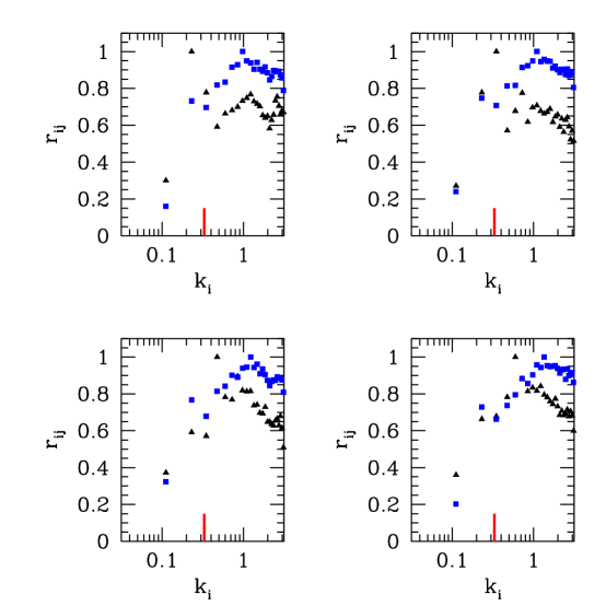
Figure 5: Correlation coefficients $r_{ij}$ from the N-body simulations as a function of $k_{i}$ for a fixed $k_{j}$. The two sets of points (triangles and squares) in each plot correspond to different $k_{j}$’s. The different values of $k_{j}$ can be deduced from the place where $r_{ij}=1$. The mark on the $x$ axis indicates the non-linear scale. The width of shells in $k$-space is $\delta k=4\pi/100$ h/Mpc.

In figure 5 we show the correlation coefficients $r_{ij}$ for different scales. Note that when both $k_{i}$ and $k_{j}$ fall well within the non-linear regime, the correlation coefficient is close to one, which implies that the power estimates at the two $k$-shells are highly correlated. The correlation coefficient decreases as the shells become further apart, but it does so very slowly. This implies that the information-gain as more modes beyond the linear regime are considered increases very slowly compared to the Gaussian expectations.

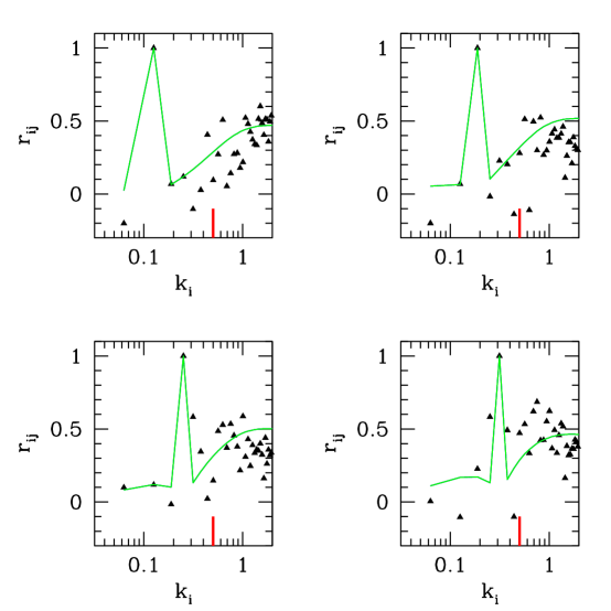
Figure 6: A comparison of $r_{ij}$ obtained from PT and N-body simulations, at $\sigma_{8}=0.375$ ($z=0.6$). Note the noise level in the covariance matrix measured from the numerical simulations; this is due to the low number (20) of realizations used to estimate the ensemble averages. The width of shells in $k$-space is $\delta k=2\pi/100$ h/Mpc.

Figure 6 shows a comparison between the correlation coefficients obtained using PT and N-Body simulations. The comparison is made at $\sigma_{8}=0.375$ ($z=0.6$), as opposed to $\sigma_{8}=0.60$ ($z=0$) in figure 5, so that more wave-modes are in the weakly non-linear regime. As one can see, there are large dispersions in the measurements of $r_{ij}$ due to the limited number of N-body simulations, but the measured values agree with the prediction of PT within the errors.

As mentioned before, the relative importance of the Gaussian versus non-Gaussian contributions to the covariance matrix depends upon the choice of binning in $k$-space. We have tested its effect with N-body simulations and the behavior is as expected from equation (4). Note that even the distinction between diagonal and off-diagonal covariances is somewhat arbitrary: by choosing a coarser binning of Fourier space, what originally appears as correlations between two nearby shells now becomes part of the diagonal variance. As is clear from equation (4), the dependence with binning becomes less important as we enter the non-linear regime.

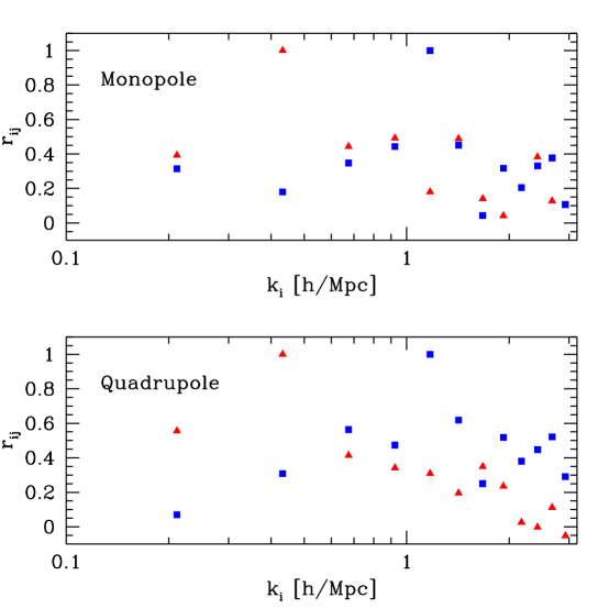
Figure 7: Cross-correlation coefficients $r_{ij}$ obtained N-body simulations in redshift space, for $\sigma_{8}=0.60$. The top panel shows $r_{ij}$ for the monopole of the power spectrum, whereas the bottom panel shows $r_{ij}$ for the quadrupole power spectrum. The width of shells in $k$-space is $\delta k=8\pi/100$ h/Mpc.

Finally, figure 7 shows correlation coefficients in redshift space. These are calculated in the plane-parallel approximation, for the same realizations shown before, in the $z=0$ output, $\sigma_{8}=0.60$. The top panel shows $r_{ij}$ for the monopole of the power spectrum, whereas the bottom panel shows $r_{ij}$ for the quadrupole moment of the power spectrum. Comparison with figure 5 shows that the effect of correlations in redshift space is somewhat suppressed with respect to the real-space clustering. That is indeed expected, since the velocity dispersion at small scales washes out clustering and therefore non-Gaussian effects.

3.3 The Power-Spectrum Covariance Matrix in the Non-Linear Regime

We now study the behavior of the power-spectrum covariance matrix in the non-linear regime, where non-Gaussian effects are most important, and compare the numerical simulations results to those predicted by the hierarchical model, which reproduces the observed scaling properties of higher-order correlations in the non-linear regime.

3.3.1 Contributions to the Covariance Matrix

It is instructive to write down the trispectrum in terms of the four-point correlation function, in order to understand the nature of the contributions to the power-spectrum covariance matrix. Writing the connected four point function $\eta_{1234}\equiv<\delta_{1}\delta_{2}\delta_{3}\delta_{4}>_{c}$, we have

$$T({\hbox{\BF k}}_{1},{\hbox{\BF k}}_{2},{\hbox{\BF k}}_{3},{\hbox{\BF k}}_{4})=\int\frac{d^{3}x_{14}}{(2\pi)^{3}}\frac{d^{3}x_{24}}{(2\pi)^{3}}\frac{d^{3}x_{34}}{(2\pi)^{3}}\ \exp{[-i({\hbox{\BF k}}_{1}\cdot{\hbox{\BF x}}_{14}+{\hbox{\BF k}}_{2}\cdot{\hbox{\BF x}}_{24}+{\hbox{\BF k}}_{3}\cdot{\hbox{\BF x}}_{34})]}\ \eta_{1234},$$ (12)

where ${\hbox{\BF x}}_{ij}\equiv{\hbox{\BF x}}_{i}-{\hbox{\BF x}}_{j}$, and due to statistical homogeneity $\eta_{1234}$ is only a function of three vectors, say ${\hbox{\BF x}}_{14}$, ${\hbox{\BF x}}_{24}$ and ${\hbox{\BF x}}_{34}$, therefore ${\hbox{\BF k}}_{4}=-{\hbox{\BF k}}_{123}$. The trispectrum configurations relevant for the covariance matrix, equation (5), then read

$$T({\hbox{\BF k}}_{1},-{\hbox{\BF k}}_{1},{\hbox{\BF k}}_{2},-{\hbox{\BF k}}_{2})=\int\frac{d^{3}x_{14}}{(2\pi)^{3}}\frac{d^{3}x_{24}}{(2\pi)^{3}}\frac{d^{3}x_{34}}{(2\pi)^{3}}\ \exp{[-i({\hbox{\BF k}}_{1}\cdot{\hbox{\BF x}}_{12}+{\hbox{\BF k}}_{2}\cdot{\hbox{\BF x}}_{34})]}\ \eta_{1234}.$$ (13)

If we restrict to the non-linear regime, where $k_{1}$ and $k_{2}$ are large, we see from Eq. (13) that this restricts $x_{12}$ and $x_{34}$ to be small; however, there is no restriction on $x_{24}$. Therefore, the power-spectrum covariance matrix in the non-linear regime receives contributions from all scales, not only those in the non-linear regime. As we shall see next, this feature takes a particular form in the context of the hierarchical model.

3.3.2 The Hierarchical Model (HM)

The hierarchical form for the trispectrum reads,

$$T({\hbox{\BF k}}_{1},{\hbox{\BF k}}_{2},{\hbox{\BF k}}_{3},{\hbox{\BF k}}_{4})=R_{a}\ [P_{1}P_{2}P_{13}+{\rm cyc.}]+R_{b}\ [P_{1}P_{2}P_{3}+{\rm cyc.}],$$ (14)

which has been proposed to explain the scaling properties of galaxy clustering in the highly non-linear regime (Fry & Peebles (1978)). In terms of the four-point function, $\eta(r)$, and the two-point function, $\xi(r)$, the hierarchical model assumes $\eta(r)\propto\xi^{3}(r)$, which implies $T\propto P^{3}$. Basically, the hierarchical model represents the trispectrum as sums of products of three power spectra, introducing only as many parameters as there are distinct topologies. The $R_{b}$ contributions (total of $4$ terms) are the “star” tree-diagrams where one vertex is connected to the other three, whereas the $R_{a}$ contributions are “snake” diagrams (total of $12$ terms). It is usually assumed that $R_{a}$ and $R_{b}$ saturate to constants independent of scale and configuration in the highly non-linear regime (and this is what we will mean by the phrase HM, except when we discuss a modified version of HM in §3.3.5). On the other hand, at large scales, PT predicts a hierarchical form for the trispectrum (equation [6]), but with $R_{a}$ and $R_{b}$ strongly dependent on configuration, as illustrated in figure 3 and figure 11 below. In our case we are interested in the configurations relevant for the power spectrum covariance matrix, equation (5), so 4 out of the 12 $R_{a}$ terms vanish, because they give $P(0)=0$. This can be potentially a problem, since in the limit that we approach these particular configurations some scales are in the linear regime, and we do not expect saturation (constant $R_{a}$ and $R_{b}$) to hold. As we shall see, this is indeed the case.

3.3.3 The Trispectrum in the HM vs. Numerical Simulations

Given the particular nature of the contributions to the power-spectrum covariance matrix, we will first discuss the validity of the HM for more general kind of configurations, were all the scales are in the non-linear regime. We have measured the trispectrum directly in the numerical simulations for configurations of four wave-vectors that form a triangle, that is, ${\hbox{\BF k}}_{1}={\hbox{\BF k}}_{2}$, and ${\hbox{\BF k}}_{3}$ at an angle $\theta$ with respect to them, for different ratios $k_{3}/k_{1}$ (${\hbox{\BF k}}_{4}=-{\hbox{\BF k}}_{123}$). In figure 8 we present two representative results, for $k_{3}/k_{1}=1.5$ and scales $k_{1}=1.26$ h/Mpc (top) and $k_{1}=1.57$ h/Mpc (bottom). The results are given in terms of the hierarchical amplitude $Q_{4}$ defined as

$$Q_{4}\equiv\frac{T_{4}({\hbox{\BF k}}_{1},{\hbox{\BF k}}_{2},{\hbox{\BF k}}_{3},-{\hbox{\BF k}}_{123})}{[P(k_{1})P(k_{2})P(k_{13})+{\rm cyc.}]+[P(k_{1})P(k_{2})P(k_{3})+{\rm cyc.}]}.$$ (15)

The lines show the predictions of hyperextended perturbation theory (HEPT),

$$Q_{4}^{\rm sat}(n)=(1/2)\ \frac{54-27\ 2^{n}+2\ 3^{n}+6^{n}}{(1+6\ 2^{n}+3\ 3^{n}+6\ 6^{n})}\equiv\frac{12R_{a}+4R_{b}}{16},$$ (16)

which gives the saturation value of the hierarchical amplitude $Q_{4}$ in the highly non-linear regime in terms of the spectral index $n=n(k)$ of the underlying linear power spectrum (Scoccimarro & Frieman 1998). The spectral index has been chosen as that of the average wave-vector at each particular configuration. HEPT only predicts the overall amplitude of $Q_{4}$; in other words, it does not attempt to model $R_{a}$ and $R_{b}$ separately. In figure 8 we show predictions for different assumptions about the relative magnitude of $R_{a}$ and $R_{b}$, $R_{a}=R_{b}$ (solid), $R_{a}=-R_{b}$ (dotted) and $5R_{a}=R_{b}$ (dashed). The trend is that as $R_{b}$ becomes smaller than $R_{a}$ (eventually becoming negative), the configuration dependence of $Q_{4}$ is opposite to that observed in the numerical simulations, where $Q_{4}$ is slightly enhanced at $\theta=0$ over its value at $\theta=\pi$. In the opposite case, when $R_{b}$ becomes larger than $R_{a}$, an increase of $R_{b}$ over $R_{a}$ gives a good fit to the N-body results, up to $R_{b}\approx 3R_{a}$. A stronger test of the HM would require to check different type of trispectrum configurations in addition to the ones we consider. Detailed testing of the HM is beyond the scope of this paper, but from these results we can conclude that at least for these type of configurations, the trispectrum in the non-linear regime agrees very well with the HM, with overall amplitude given by HEPT and weights $R_{a}\approx R_{b}$.

3.3.4 The Power-Spectrum Covariance Matrix in the HM

We now consider the calculation of the power-spectrum covariance matrix in the HM, and show that it leads to unphysical results for the cross-correlation coefficient in the limit that shells are widely separated.

In order to get the bin-averaged trispectrum, equation (5), we need to integrate over the angle between the two wave-vectors in the two shells under consideration. It is clear that if, say, $k_{2}\gg k_{1}$, then $\int_{-1}^{1}(dx/2)\ P(|{\hbox{\BF k}}_{2}-{\hbox{\BF k}}_{1}|)\approx P(k_{2})$. It turns out, however, that in practice this approximation works quite well in the non-linear regime even for $k_{1}=k_{2}$. Thus, we get simple approximate expressions for the diagonal and off-diagonal contributions of the bin-averaged trispectrum

$${\bar{T}}(k_{i},k_{i})\approx 4(2R_{a}+R_{b})\ P_{i}^{3}.$$ (17)

$${\bar{T}}(k_{i},k_{j})\approx 2(R_{a}+R_{b})\ P_{i}P_{j}^{2}+2(2R_{a}+R_{b})\ P_{i}^{2}P_{j}+2R_{a}\ P_{i}^{3},$$ (18)

where we have assumed that $k_{i}>k_{j}$, and that $R_{a}$ and $R_{b}$ are constants independent of configuration. These expressions turn out to agree with results of numerical integrations over shells to about $3\%$ for the whole range of $k_{1}$ and $k_{2}$. Note that equation (18) reduces to equation (17) in the limit that $k_{i}\rightarrow k_{j}$. These expressions imply that in the limit where the non-Gaussian contribution to the covariance matrix dominates ($k_{i}>k_{j}$)

$$r_{ij}\approx\frac{(R_{a}+R_{b})}{2(2R_{a}+R_{b})}\times\sqrt{\frac{P_{j}}{P_{i}}}.$$ (19)

This result implies that, unless $R_{a}=-R_{b}$, eventually as $k_{i}\gg k_{j}$ the cross-correlation coefficient $r_{ij}$ becomes larger than unity, which is unphysical. As shown in figure 8 a constant relation $R_{a}=-R_{b}$ is not a good fit to the N-body results on general trispectrum configurations. Furthermore, it turns out that a constant relation $R_{a}=-R_{b}$ is inconsistent with the numerical results presented in Section 3.2, since it predicts that $r_{ij}$ decays much faster with shell separation than what is observed in the numerical simulations. We therefore conclude that a hierarchical model with amplitudes $R_{a}$ and $R_{b}$ independent of scale and configuration is actually not a good description of the power-spectrum covariance matrix in the non-linear regime.

3.3.5 HM Predictions vs. N-body Simulations for the Covariance Matrix

Given the results in the previous sections, we expect to find deviations from the HM predictions for the power-spectrum covariance matrix in the non-linear regime. We now explore the nature of these deviations by comparing with numerical simulations and use both PT and the HM as a tool to understand the results.

The first non-trivial test is the scaling of diagonal elements. Both PT and the HM predict that the diagonal part of the trispectrum must scale as the third power of the power spectrum, equations (9) and (17). Therefore, even though the covariance matrix in the non-linear regime receives contributions from a range of scales according to equation (13), one expects the HM scaling to be correct. As shown in figure 4a, the HM scaling (solid lines) agrees with the numerical simulations (symbols). However, we find that the overall amplitude is a factor of five times smaller than that predicted by equation (16) for $R_{a}\approx R_{b}$. This suppression must come from the range of scales (including large ones) that contribute in equation (13), and therefore it is difficult to explain quantitatively without a full description of the four-point function.

Figure 9 shows a more detailed comparison of HM predictions with the cross-correlation coefficients $r_{ij}$ measured in the N-body simulations. In this calculation, we have assumed $R_{a}=R_{b}$ with $Q_{4}^{\rm sat}(n)$ as given by HEPT. Note the very good agreement, especially around $k_{i}\approx k_{j}$. As $k_{i}$ gets much larger than $k_{j}$ we see that the predicted $r_{ij}$ start to increase, a signature that the condition $R_{a}\approx R_{b}$ is breaking down, as discussed above.

In light of these results, we will now use a HM with arbitrary functions $R_{a}$ and $R_{b}$, and explore the behavior of these functions implied by our N-body measurements. Note that once we give up the hypothesis that $R_{a}$ and $R_{b}$ are strictly constants, we should distinguish between two kinds of $R_{a}$ and $R_{b}$: the $R_{a}$ and $R_{b}$ in equation (14) which depend on both configuration and scale, and the effective $R_{a}$ and $R_{b}$ in equations (17-18) which have the configuration dependence integrated out. We will rely on the context to differentiate between the two meanings here.

Given our measurements of the power spectrum covariance matrix presented in Section 3.2, we can obtain estimates for $R_{a}$ and $R_{b}$ from equations (17-18). However, since the largest contribution is due to the first term in equation (18), the best constraint is on the average value, $(R_{a}+R_{b})/2$. This is shown in figure 10, for the particular case of $k_{j}=0.98$ h/Mpc as a function of $k_{i}$. We see that the average value shows a systematic decrease with shell separation. Since this configuration dependence is likely to come from scales not in the non-linear regime, it is useful to consider PT, which predicts a specific relation between $R_{a}$ and $R_{b}$ as a function of shell separation, to see whether we can explain the decline in figure 10.

In figure 11 we show the ratio $R_{b}/R_{a}$ predicted by PT as a function of configuration angle $\theta$ between ${\hbox{\BF k}}_{1}$ and ${\hbox{\BF k}}_{2}$ for different scales. We see that for shells close to each other, although the ratio $R_{b}/R_{a}$ varies, on average $R_{a}\approx R_{b}$ (in fact, for $k_{1}=k_{2}=1$ h/Mpc, the angular average yields $R_{a}\approx 1.5R_{b}$). However, as the shells become more separated, the averaged relation between $R_{a}$ and $R_{b}$ changes, reaching $R_{a}=-R_{b}$ in the limit of large separation, just what is needed in a hierarchical model to preserve the condition that the cross-correlation coefficient $r_{ij}\leq 1$.

We now examine whether the type of configuration dependence valid in PT can explain the behavior of $(R_{a}+R_{b})/2$ deduced from the N-body results. In figure 10, the solid line shows the prediction for $(R_{a}+R_{b})/2$ as a function of shell separation assuming that the averaged relation between $R_{a}$ and $R_{b}$ is the same as that given by PT. The overall amplitude has been chosen to fit the diagonal values, at $k_{i}=k_{j}=0.98$ h/Mpc. We see that this prediction works quite well to explain the configuration dependence of the covariance matrix in the non-linear regime.

3.3.6 Summary

To summarize, we found that the hierarchical model (HM) is not a valid description of the power-spectrum covariance matrix in the non-linear regime. Instead, we find that the covariance matrix behaves as a “generalized” HM with a configuration dependence that resembles that in PT. We interpret this as a consequence of the fact that even in the non-linear regime the covariance matrix receives contributions from large scales. On the other hand, we have tested the HM for other trispectrum configurations in the non-linear regime and found good agreement for $R_{a}\approx R_{b}$ and overall amplitude given by HEPT.

Although N-body results have been restricted to the SCDM model, it is worth mentioning that hierarhical amplitudes such as $Q_{4}$, $R_{a}$ and $R_{b}$ are expected to be very insensitive to cosmological parameters, as can be shown quite generally from the equations of motion of gravitational instability (Scoccimarro et al. 1998, Appendix B.3). Therefore, we expect that the dependence of the covariance matrix on cosmology will appear only through the overall dependence on the power spectrum.

4 Impact on Cosmological Parameter Determination

To assess the importance of the non-Gaussian terms in the covariance matrix, suppose we are interested in only one parameter: the amplitude of the power spectrum over a range of scales. Let us assume that the shape, $\bar{P}(k_{i})$, is known and let us estimate the amplitude $x=P(k_{i})/\bar{P}(k_{i})$. If only the Gaussian terms of the covariance were important, the minimum variance estimator for the amplitude would be,

$$\hat{x}={\sum_{k_{i}<k_{\rm max}}N_{k_{i}}\hat{P}(k_{i})/\bar{P}(k_{i})\over\sum_{k_{i}<k_{\rm max}}N_{k_{i}}},$$ (20)

where we simply weigh the power in each bin by its inverse variance, and all bins are used up to some $k_{\rm max}$. In the same Gaussian limit the variance of $\hat{x}$ would be

$$\sigma_{x}^{2}=\langle\hat{x}^{2}\rangle-\langle\hat{x}\rangle^{2}={2\over N_{t}},$$ (21)

where $N_{t}=\sum N_{k_{i}}$ is the total number of $k$ modes used.

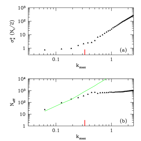
Figure 13: Panel (a) shows the variance of $\hat{x}$ measured using the N-body simulations. Panel (b) shows the effective number of modes. The results are for $\sigma_{8}=0.60$ ($z=0$) and the non-linear scale is shown with a mark on the $x$ axis.

Figure 12 shows the ratio $\sigma_{x}^{2}/(2/N_{t})$ obtained using perturbation theory for a 1 Gpc/h box. On large scales, $k_{\rm max}\,\mbox{${}^{<}_{\sim}$}\,0.1$ h/Mpc, PT shows that the non-Gaussian contributions do not have a significant impact on the determination of $x$, the error-bar starts increasing rapidly thereafter (for this cosmological model $k_{nl}=0.33$ h/Mpc, and at the smoothing scale of $R\sim 1/k_{nl}$, $S_{4}\sigma^{2}/5$ is of order 1). In figure 13a, we show the corresponding results from N-body simulations. In figure 13b we show the effective number of modes, defined as $N_{\rm eff}\equiv 2/\sigma_{x}^{2}$. As we can see, $N_{\rm eff}$ varies much more slowly once we enter the non-linear regime.

In the non-linear regime, different band-power estimates become highly correlated. What this means in practice is that the power at different bands fluctuate up and down together, making the overall amplitude of the power spectrum difficult to determine while essentially preserving information on its shape. This can be made more precise by considering the following covariance matrix:

$$C_{ij}=\beta[P_{i}P_{j}]^{3\over 2}(1-\epsilon_{ij})$$ (22)

which follows from equation (4), ignoring the Gaussian term, and from equation (17). The parameter $\beta$ is some simple constant proportional to $V_{f}$. The symmetric matrix $\epsilon_{ij}$ has vanishing diagonal elements, $\epsilon_{ii}=0$, and the off-diagonal elements determine the cross-correlations between different band-powers. We will consider the limit in which $\epsilon_{ij}$ is small (see figure 9), in other words all modes are highly correlated and $C_{ij}$ is nearly singular. Furthermore, as is clear from figure 9, $\epsilon_{ij}$ is slowly varying, and we will treat $\epsilon_{ij}=\epsilon$ as a constant.

Let us consider the following rescaling of the power spectrum estimate:

$$\hat{y}_{i}={\hat{P}_{i}\over{{\sqrt{\beta}}[P_{i}]^{3/2}}}.$$ (23)

where the true power spectrum $P(k_{i})$ is of course unknown a priori, but one can think of it instead as a fiducial power spectrum and we are trying to measure deviations from it. (It is actually not necessary to make this change of variable at all, but it will simplify some of our expressions below.) The corresponding covariance matrix is then

$$C^{y}_{ij}=\langle\hat{y}_{i}\hat{y}_{j}\rangle-\langle\hat{y}_{i}\rangle\langle\hat{y}_{j}\rangle=1-\epsilon\ (1-\delta_{ij})$$ (24)

We can diagonalize this matrix and ask which combinations of the band powers are better determined (see Hamilton 1997b for other choices of rescaling and diagonalization). There are two types of eigenvalues. The first is $\lambda_{1}=N-(N-1)\epsilon$, associated with the eigenvector ${\hbox{\boldmath{$e$}}}_{1}=(1,1,1,....,1)/\sqrt{N}$, where $N$ is the number of bands. This eigenvector corresponds to the overall amplitude of the rescaled power spectrum. In addition, there are $N-1$ degenerate eigenvectors, each with an eigenvalue $\lambda=\epsilon$. The corresponding eigenvectors are ${\hbox{\boldmath{$e$}}}_{m}=(0,0,...1,-1,0...,0)/\sqrt{2}$, where the $1$ is in the $m-1$-th position ($m=2,...,N$). Each of these eigenvectors provides a measure of the local derivative of the rescaled power spectrum. Note that the above set of eigenvectors are linearly independent but do not form an orthogonal basis. In the case where $\epsilon$ (or more precisely $\epsilon_{ij}$) actually varies slowly with the band, but still remains small, the above conclusions remain largely unchanged: $\lambda_{1}=N+O(\epsilon_{ij})$, and the rest of the eigenvalues satisfy $\lambda\sim\epsilon$ ($\epsilon_{ij}\sim\epsilon$ plus small variations) except that the degeneracy is lifted by the slowly varying $\epsilon_{ij}$.

Clearly, $\lambda_{1}$ is much larger than any other eigenvalues. Hence, the combination corresponding to ${\hbox{\boldmath{$e$}}}_{1}$ is the most poorly determined. To be more precise, the fractional error in the quantity $\hbox{\boldmath{$\hat{y}$}}\cdot\hbox{\boldmath{$e$}}_{1}$ is

$$\sqrt{\langle[\hbox{\boldmath{$\hat{y}$}}\cdot\hbox{\boldmath{$e$}}_{1}-\langle\hbox{\boldmath{$\hat{y}$}}\cdot\hbox{\boldmath{$e$}}_{1}\rangle]^{2}\rangle\over\langle\hbox{\boldmath{$\hat{y}$}}\cdot\hbox{\boldmath{$e$}}_{1}\rangle^{2}}=(1+O(\epsilon))\left[{1\over N}\sum_{i}{1\over\sqrt{\beta P_{i}}}\right]^{-1}\,.$$ (25)

To the extent that $\sqrt{P(k_{i})}$ is slowly varying with $k_{i}$, the fractional error is approximately independent of $N$, which means increasing the number of bands does not help reduce the error in this estimate of the amplitude of the rescaled power spectrum. The only way to reduce the error is to make $\beta$ smaller, i.e. having a larger survey volume.

On the other hand, the local spectral index of the rescaled power spectrum can be defined as $\hbox{\boldmath{$\hat{y}$}}\cdot\hbox{\boldmath{$e$}}_{m}/\langle\hat{y}_{m}\rangle$ ($m\neq 1$), and its error is given by (we use error instead of fractional error here because the local spectral index could vanish):

$${\sqrt{\langle[\hbox{\boldmath{$\hat{y}$}}\cdot\hbox{\boldmath{$e$}}_{m}-\langle\hbox{\boldmath{$\hat{y}$}}\cdot\hbox{\boldmath{$e$}}_{m}\rangle]^{2}\rangle}\over\langle\hat{y}_{m}\rangle}=\sqrt{\epsilon\beta P_{m}}$$ (26)

which is $O(\sqrt{\epsilon})$ smaller than the error in the rescaled amplitude. It is intriguing that even though only two neighboring bands are required to estimate the shape while all bands are used to estimate the amplitude, it is the former that is better determined. This is a result of the high correlation limit that we have taken, which makes averaging over band-powers nearly useless.

5 Covariance Matrix of the Projected Power Spectrum: Application to Weak Lensing

We shall now consider the statistics of the (2D) projected density field. Suppose one observes a small patch of the sky covering a solid angle $\Omega$. The patch is taken to be small enough that we can use the flat sky approximation and expand the projected mass density in Fourier modes instead of spherical harmonics. We will consider

$$\kappa(\hbox{\boldmath{$\theta$}})=\int_{0}^{\chi_{0}}d\chi\ w(\chi)\ \delta(r(\chi)\theta_{x},r(\chi)\theta_{y},\chi),$$ (27)

where $w(\chi)$ is a slowly varying function of the radial comoving distance to the observer $\chi$. We introduce the angular-diameter distance $r(\chi)$, $r(\chi)=K^{-1/2}\sin K^{-1/2}\chi,\chi,(-K)^{-1/2}\sinh(-K)^{-1/2}\chi$ for models with positive, zero and negative curvature respectively, and $K=(\Omega_{0}-1)H_{0}^{2}$ with $H_{0}$ the present value of the Hubble constant. For weak-lensing the relevant weight function $w(\chi)$ is

$$w(\chi) = {3\over 2}H_{0}^{2}\Omega_{m}{g(\chi_{0},\chi)\over a}$$

$$g(\chi,\chi^{\prime}) = {r(\chi^{\prime})\ r(\chi-\chi^{\prime})\over r(\chi)}\,,$$ (28)

in which case $\kappa$ is the weak-lensing convergence for background galaxies located at $\chi=\chi_{0}$. Note that our definition of $\kappa$ here is a factor of 2 larger than the one commonly used (see e.g. Jain et al. 1999). We are interested in the Fourier components of the projected field, from equation (27) we obtain

$$\kappa(\hbox{\boldmath{$l$}})=\int{d^{2}{\hbox{\boldmath{$\theta$}}}\over(2\pi)^{2}}\ e^{-i{\hbox{\boldmath{$l$}}}\cdot{\hbox{\boldmath{$\theta$}}}}\ \kappa(\hbox{\boldmath{$\theta$}})=\int d\chi\frac{w(\chi)}{r^{2}(\chi)}\ \int_{-\infty}^{\infty}dk\ \delta\Big{(}\frac{\hbox{\boldmath{$l$}}}{r(\chi)},k\Big{)}\ e^{ik\chi},$$ (29)

which gives the two-point correlator

$$\mathop{\langle}\kappa(\hbox{\boldmath{$l$}})\kappa(\hbox{\boldmath{$l$}}^{\prime})\mathop{\rangle}=\int d\chi_{1}\ \frac{w_{1}}{r_{1}^{2}}\int d\chi_{2}\ \frac{w_{2}}{r_{2}^{2}}\ \delta_{\rm D}\Big{(}\frac{\hbox{\boldmath{$l$}}}{r_{1}}+\frac{\hbox{\boldmath{$l$}}^{\prime}}{r_{2}}\Big{)}\times\int_{-\infty}^{\infty}dk\ e^{ik(\chi_{1}-\chi_{2})}\ P[\sqrt{(l^{2}/r_{1}^{2})+k^{2}}]\,$$ (30)

where $w_{i}\equiv w(\chi_{i})$ and similarly $r_{i}\equiv r(\chi_{i})$. The integral over the line-of-sight wave-vector is dominated by $k(\chi_{1}-\chi_{2})\equiv k\Delta\chi\mathrel{\mathchoice{\lower 3.6pt\vbox{\halign{$\mathsurround=0pt\displaystyle\hfill#\hfil$\cr<\crcr\sim\crcr}}}{\lower 3.6pt\vbox{\halign{$\mathsurround=0pt\textstyle\hfill#\hfil$\cr<\crcr\sim\crcr}}}{\lower 3.6pt\vbox{\halign{$\mathsurround=0pt\scriptstyle\hfill#\hfil$\cr<\crcr\sim\crcr}}}{\lower 3.6pt\vbox{\halign{$\mathsurround=0pt\scriptscriptstyle\hfill#\hfil$\cr<\crcr\sim\crcr}}}}1$, where $\Delta\chi$ must be the typical scale of variation of $w(\chi)/r(\chi)^{2}$ (otherwise the total integration vanishes). In the small angle approximation, it is reasonable to assume that over the scales of interest $w(\chi)/r(\chi)^{2}$ is approximately constant, that is, $l/r\gg 1/\Delta\chi$. Therefore, $l^{2}/r_{1}^{2}\gg k^{2}$, i.e. only perpendicular Fourier modes contribute to the projected field, then $P(\sqrt{l^{2}/r_{1}^{2}+k^{2}})\approx P(l/r_{1})$ and the integral over $k$ gives a delta function in $\Delta\chi$. Thus, we obtain

$$\mathop{\langle}\kappa(\hbox{\boldmath{$l$}})\kappa(\hbox{\boldmath{$l$}}^{\prime})\mathop{\rangle}=(2\pi)\ \delta_{\rm D}({\hbox{\boldmath{$l$}}}+{\hbox{\boldmath{$l$}}^{\prime}})\ \int d\chi\ \frac{w^{2}(\chi)}{r^{2}(\chi)}\ P[l/r(\chi)],$$ (31)

which is nothing but Limber’s equation (Peebles (1980); Kaiser (1992, 1998)). The power spectrum estimator for the projected density field is accordingly

$${\hat{P}}_{\kappa}(l_{i}) = A_{f}\int_{l_{i}}{d^{2}{\hbox{\boldmath{$l$}}}\over A_{r}(l_{i})}\ \kappa({\hbox{\boldmath{$l$}}})\kappa(-{\hbox{\boldmath{$l$}}}),$$ (32)

where $A_{f}=(2\pi)^{2}/\Omega$ is the area of the fundamental cell in $l$ space, and we have assumed an average over a ring in $l$-space with area $A_{r}(l_{i})$ and centered at $l_{i}=i\times\delta l$. Equations (31) and (32) lead to

$$\langle\hat{P}_{\kappa}(l)\rangle = (2\pi)\int d\chi{w^{2}(\chi)\over r^{2}(\chi)}P[l/r(\chi)].$$ (33)

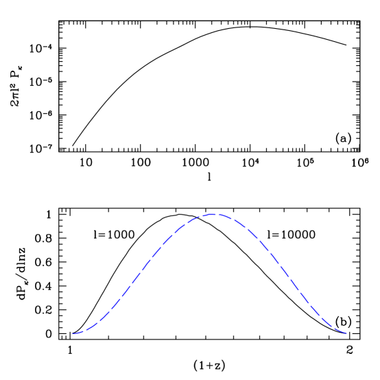
Figure 14: Panel (a) shows the power spectrum of the projected mass density for the cluster-normalized SCDM model. The sources are assumed to be located at $z=1$. The bottom panel illustrates where the contribution is coming from in redshift. The area under the curve is proportional to the projected power spectrum, the normalization is arbitrary.

In figure 14a we show the power spectrum for the weak-lensing convergence assuming that the background galaxies are at a redshift of $z=1$. Following Jain & Seljak (1997), we use a model of the non-linear power spectrum proposed by Hamilton et al. (1991), and later extended by Peacock & Dodds (1994,1996) and Jain et al. (1995). In panel b we show the integrand of equation (33) as a function of redshift for $l=1000$ and $l=10000$. The area under the curve is proportional to $P_{\kappa}$. We conclude that the peak contribution comes from $z=0.3-0.4$ depending on the $l$ of interest, but that the integrand is a very broad function of redshift.

The previous calculation can be easily extended to higher moments of the projected field. We obtain

$$\langle\kappa(\hbox{\boldmath{$l$}}_{1})\cdots\kappa(\hbox{\boldmath{$l$}}_{n})\rangle_{c}=(2\pi)^{n-1}\delta_{\rm D}(\hbox{\boldmath{$l$}}_{1}+\cdots+\hbox{\boldmath{$l$}}_{n})\ \int d\chi\ {w^{n}(\chi)\over r^{2n-2}(\chi)}\ T_{n}[\hbox{\boldmath{$l$}}_{1}/r(\chi),\cdots,\hbox{\boldmath{$l$}}_{n}/r(\chi)].$$ (34)

Equations (32) and (34) can be used to calculate the covariance matrix of the power spectrum estimator,

$$C_{ij} = A_{f}\ [{2P_{\kappa}^{2}(l_{i})\over A_{r}(l_{i})}\delta_{ij}+\bar{T}_{\kappa}(l_{i},l_{j})]$$

$$\bar{T}_{\kappa}(l_{i},l_{j}) \equiv (2\pi)^{3}\int d\chi{w^{4}(\chi)\over r^{6}(\chi)}\int_{l_{i}}{d^{2}{\hbox{\boldmath{$l$}}}_{1}\over A_{r}(l_{i})}\int_{l_{j}}{d^{2}{\hbox{\boldmath{$l$}}}_{2}\over A_{r}(l_{j})}T[\hbox{\boldmath{$l$}}_{1}/r(\chi),-\hbox{\boldmath{$l$}}_{1}/r(\chi),\hbox{\boldmath{$l$}}_{2}/r(\chi),-\hbox{\boldmath{$l$}}_{2}/r(\chi)].$$ (35)

Before presenting the results of the numerical evaluation of the different terms in equation (35), we will make an order of magnitude estimate of the size of the different terms. In the process, we hope to gain some physical insight and understand how the different terms scale with the parameters of the problem. The ratio of the non-Gaussian to Gaussian terms is (for $i=j$)

$${\cal R}={A_{r}\bar{T}_{\kappa}\over 2P_{\kappa}^{2}}.$$ (36)

We then make the following crude approximations:

$$P_{\kappa}(l) \approx (2\pi)\Delta\chi^{*}\ {w^{2}(\chi^{*})\over r(\chi^{*})^{2}}\ P[l/r(\chi^{*})]\,,$$

$$\bar{T}_{\kappa}(l,l) \approx (2\pi)^{3}\Delta\chi^{*}\ {w^{4}(\chi^{*})\over r(\chi^{*})^{6}}\ \bar{T}[l/r(\chi^{*}),l/r(\chi^{*})]\,,$$ (37)

where we have assumed that the line of sight integral is dominated by contributions from $\chi^{*}\pm\Delta\chi^{*}/2$, and that the integrand remains roughly constant over this interval. We neglect the configuration dependence of the trispectrum and just use its typical value at the scale of interest. Note that both the power spectrum and the trispectrum are a function of time so they should be evaluated at $\chi^{*}$. Under these simplifying assumptions the ratio becomes

$${\cal R}={\pi A_{r}\over r^{2}(\chi^{*})\Delta\chi^{*}}{\bar{T}\over P^{2}}.$$ (38)

It is interesting to compare these formulae with their analogues in 3D (equation [4]). If we make the identification $k=l/r(\chi^{*})$, $\Delta k_{\chi}=2\pi/\Delta\chi^{*}$ and $\delta k=\delta l/r(\chi^{*})$, we can rewrite the prefactor ${\pi A_{r}/r^{2}(\chi^{*})\Delta\chi^{*}}$ as $2\pi k\Delta k_{\chi}\delta k/2$. Let’s compare this with the relevant prefactor in the 3D case: $4\pi k^{2}\delta k/2$. By assumption, $k\gg\Delta k_{\chi}$, which means that the Gaussian variance is much larger, or the ratio of non-Gaussian to Gaussian terms is much smaller, in 2D compared to 3D. This is a result of the fact that only the Fourier modes perpendicular to the line of sight contribute to the 2D projection, by virtue of an otherwise rapidly oscillating integrand (see derivation above). This means a far fewer number of non-linear modes are available in 2D compared to 3D, for a given $k$. While in 3D all the modes in a shell of volume $4\pi k^{2}\delta k$ are available, in 2D only those in a ring-shaped region of area $2\pi k\delta k$ and height $\Delta k_{\chi}$ contribute to non-Gaussianity. Hence, projection raises the significance of the Gaussian variance relative to the non-Gaussian term.

The projection has another interesting effect. As discussed in the context of the hierarchical ansatz, the trispectrum scales as the third power of the power spectrum. Contrary to what happens for the three-dimensional case, the number of modes only increases like $k^{2}=l^{2}/r^{2}(\chi)$ as we go to higher $l$ (we are assuming $\delta l\sim l$ here as it gives the correct order of magnitude estimate of the true significance of non-Gaussian terms). The ratio $\cal R$ scales as ${\cal R}\propto{k^{2}P(k)/\Delta\chi^{*}}$ instead of $k^{3}P(k)$ for the 3D case. As a consequence, if the 3D power spectrum decreases faster than $k^{-2}$, the relative importance of the non-Gaussian variance can actually decrease as one goes to smaller angular scales.

As an example we consider the weak-lensing effect on background galaxies at a redshift of $z\sim 1$. We then take $\chi^{*}$ corresponding to a redshift of $z\sim 0.4$, which means a distance of $r(\chi^{*})=\chi^{*}\sim 1{\,\rm h^{-1}Gpc}$. Because the integrand is a slowly varying function of $\chi$ we will take $\Delta\chi^{*}\sim\chi^{*}$. We will concentrate on scales $l>1000$ ($\theta<1/l\approx 3^{{}^{\prime}}$ in the correlation function) which at this distance correspond to $k>1$ h/Mpc. Since these scales are all in the non-linear regime, to estimate the magnitude of $\cal R$ we use the value of the trispectrum obtained in the simulations, ${\bar{T}}\sim 17P^{3}$, to get

$${\cal R}\sim 0.2\ \Big{(}{l\over 1000}\Big{)}\ \Big{(}{\delta l\over 1000}\Big{)}\Big{(}{1{\,\rm h^{-1}Gpc}\over r(\chi)}\Big{)}^{2}\Big{(}{1{\,\rm h^{-1}Gpc}\over\Delta\chi}\Big{)}\Big{(}{\bar{T}/P^{3}\over 17}\ {P(l/1{\,\rm h^{-1}Gpc})\over{0.5{\,\rm h^{-3}Mpc^{3}}}}\Big{)}$$ (39)

This is in contrast with the 3D case where the corresponding $\cal R$ is larger than $1$ for $k>1$ h/Mpc. As we said above, projection decreases the effective number of non-linear modes which makes the Gaussian variance comparatively more important.

We can compare our estimate of $\cal R$ with other measures of non-Gaussianity in simulations of weak lensing. Jain et al. (1999) computed the skewness of $\kappa$ and found $S_{3}\sigma\approx 1.6$ on a scale of $3^{{}^{\prime}}$. To make the connection with our result we will assume that this number also estimates $S_{4}\sigma^{2}$, as expected by simple scaling. Then we note that $S_{4}\sigma^{2}$ can be written as,

$$S_{4}(R)\sigma^{2}=\frac{\int d^{2}l_{1}d^{2}l_{2}d^{2}l_{3}\ W_{1}W_{2}W_{3}W_{123}\ T_{\kappa}(\hbox{\boldmath{$l$}}_{1},\hbox{\boldmath{$l$}}_{2},\hbox{\boldmath{$l$}}_{3},-\hbox{\boldmath{$l$}}_{123})}{[\int d^{2}l\ W^{2}(lR)\ P_{\kappa}(l)]^{2}},$$ (40)

where $W_{i}\equiv W(l_{i}R)$, with $W$ being the Fourier transform of the smoothing window. We see that $S_{4}\sigma^{2}$ measures the same ratio of trispectrum and power spectrum that is relevant for $\cal R$ but with one caveat. $S_{4}\sigma^{2}$ is determined by an average over all trispectrum configurations while $\cal R$ is sensitive to those particular shapes relevant for the covariance matrix, and as we discussed in §3.3.5, the latter is smaller than the naive expectation by a factor of five. Thus we expect $S_{4}\sigma^{2}/5$ to be comparable to $\cal R$, as indeed it is.

Also note that the weight function $w(\chi)$ cancels out in the ratio $\cal R$, so the above conclusions apply equally well to other types of projection, such as that in angular galaxy surveys. The non-Gaussian contribution to the error is comparable but does not dominate over the Gaussian contribution for the cluster-normalized SCDM model, and for mass distributions projected over cosmological distances ($\sim 1{\,\rm h^{-1}Gpc}$). For angular surveys, however, the effects of non-Gaussianity are likely to be larger than in the weak-lensing case, since the projection takes place over a smaller range of scales.

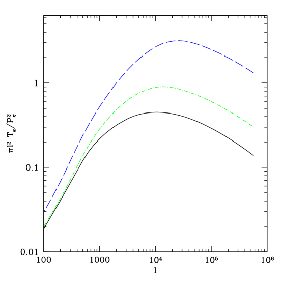
Figure 15: Ratio of the non-Gaussian to Gaussian terms in the covariance of the projected mass density, for cluster-normalized SCDM (solid line), $\Lambda$CDM (dot-dashed line) and open CDM (dashed line) models. The hierarchical ansatz was assumed in the calculation, with $R_{a}\approx R_{b}$. See text for details.

In figure 15 we show the result of numerically integrating equation (35). We use here the hierarchical form together with HEPT discussed in §3.3, but rescale the amplitude of $R_{a}$ ($\approx R_{b}$) to match the amplitude of the power spectrum variance measured in the simulations ($T/P^{3}=17$ at $k=1{\,\rm{hMpc^{-1}}}$ for the SCDM model). The figure shows the ratio of the diagonal terms of the covariance so this value is all that is needed to normalize the calculation. This should be a good approximation for most of the scales shown, but would start to break down close to $l\sim 100$, in which case the PT result would begin to take over (see equation 9). We show the results for three cosmological models, the SCDM model we have been considering so far ($\sigma_{8}=0.60,\ \Gamma=0.5$), an open model with $\Omega_{m}=0.3$, $\Gamma=0.21$ and $\sigma_{8}=0.85$, and a flat cosmological constant ($\Lambda$) dominated model with $\Omega_{m}=0.3$ and $\Omega_{\Lambda}=0.7$. We have assumed the the hierarchical ratios $R_{a}$ and $R_{b}$ are independent of the cosmological model, which should hold to a very good approximation (Scoccimarro et al. (1998)).

The ratio $\cal R$ obtained in the numerical integration for SCDM is in agreement with our simple estimate in equation (39). Furthermore we can see that the ratio has a maximum around $l\approx 8000$, which is a consequence of the fact that the 3D power spectrum decreases faster than $k^{-2}$ therefater. Even though we are probing scales that are more non-linear as we go to higher $l$, the projection actually makes the estimates of the power spectrum of $\kappa$ more Gaussian, since the number of non-linear modes does not increase as fast as to compensate for the decaying power spectrum. Therefore, contrary to what happens in 3D, the non-Gaussian effects never dominate even at very small scales for the SCDM model.

Figure 15 shows that the non-Gaussian effects can be more important in other models, however. The main difference between models arises due to their different normalizations, parametrized by $\sigma_{8}$ (in all cases, the normalization is chosen to yield the correct cluster abundance today). An additional effect which enhances the signature in the open model is the difference in the fluctuation growth rates. The parameter $\sigma_{8}$ specifies the normalization at the present time but the lensing effect is sensitive to the amplitude of the fluctuations all the way up to the redshift of the background galaxies. In the open model structure grows slower than in the flat one, so for a given normalization today the average power up to a redshift $z\sim 1$ is significantly larger. The growth rate of the cosmological constant model is intermediate between that of the open and flat models. Hence, although the open and cosmological constant models have the same present normalization, the size of the ratio in figure 15 differs for the two models. Finally, there is one more differentiating factor: the angular-diameter distance to the relevant redshifts is largest in the $\Lambda$ model, which tends to further reduce $\cal R$ (equation [39]).

Our results for different cosmologies agree roughly with the numerical investigations carried out by van Waerbeke et al. (1998). We generally find, however, a smaller (by a factor of order two) non-Gaussian contribution than they do. The source of this discrepancy is likely the different treatment of the dynamics of gravitational clustering. As described above, we use as an approximation the hierarchical model for the diagonal non-Gaussian contribution; on the other hand, van Waerbeke et al. (1998) use the dynamics of second-order Lagrangian perturbation theory in 2D.

In summary, we have shown that the non-Gaussian terms in the diagonal of the projected power spectrum, which arise due to the non-linear nature of gravitational clustering, can be the dominant source of error in some models, depending on the normalization and cosmology. These terms should be included when analyzing future surveys or when trying to predict their capabilities (van Waerbeke et al. (1999); Hu & Tegmark (1998)). Perhaps more importantly, as in the three-dimensional case, gravitational clustering induces correlations between different band-powers, in addition to increasing their individual error-bars. Calculations similar to those performed for figure 9 are straightforward to carry out for weak-lensing, but will not be included here.

6 Discussion

We have analyzed the covariance matrix for band-power estimates, both for the three-dimensional matter density and its angular projection. Three general statements can be made. First, the non-linear nature of gravitational clustering tends to increase the diagonal variance over the Gaussian error as well as induce correlations between different band-powers. Second, for scales $k$ where $4\pi k^{3}P(k)\mathrel{\mathchoice{\lower 3.6pt\vbox{\halign{$\mathsurround=0pt\displaystyle\hfill#\hfil$\cr<\crcr\sim\crcr}}}{\lower 3.6pt\vbox{\halign{$\mathsurround=0pt\textstyle\hfill#\hfil$\cr<\crcr\sim\crcr}}}{\lower 3.6pt\vbox{\halign{$\mathsurround=0pt\scriptstyle\hfill#\hfil$\cr<\crcr\sim\crcr}}}{\lower 3.6pt\vbox{\halign{$\mathsurround=0pt\scriptscriptstyle\hfill#\hfil$\cr<\crcr\sim\crcr}}}}1$, the covariance matrix is reasonably well approximated by its Gaussian part; conversely, the Gaussian approximation rapidly breaks down on scales $4\pi k^{3}P(k)\,\mbox{${}^{>}_{\sim}$}\,1$. Third, and interestingly, band-powers on non-linear scales are actually significantly correlated with band-powers on quasilinear scales (see e.g. figure 2); this is because the growth of wave modes on small scales is significantly affected by the presence of long-wave modes.

We have also discussed how the relative importance of Gaussian and non-Gaussian terms is somewhat dependent upon the choice of binning in $k$-space, because the binning affects the Gaussian covariance but not the non-Gaussian one (equation [4]). Coarse graining in $k$-space lowers the Gaussian variance, while increasing the survey size decreases the overall amplitude of the covariance matrix. However, there are binning-independent ways to quantify the relative importance of non-Gaussian versus Gaussian variances, such as by focusing on the estimation of the amplitude of the power spectrum (see §4). In this particular case, one is essentially using a very coarse bin which includes all wave-modes. This is the reason why simple estimates such as the one given in equation (40) work as a rough guide as to the importance of non-Gaussianity. In the highly non-linear regime where all wave modes are highly correlated, the amplitude of a rescaled power spectrum (equation [23]) is more poorly determined compared to its shape. The key to decreasing error-bars in this case is to increase the survey volume, rather than adding more wave-bands.

Angular projection adds interesting new twists to the above general picture. We have studied the projection relevant for weak lensing in more detail, but most of our conclusions should hold for other projections as well since the relevant weight function $w(\chi)$ (equation [27]) drops out of the non-Gaussian-to-Gaussian ratio $\cal R$ (equation [38]). Projection tends to reduce the relative importance of non-Gaussianity, as fewer non-linear modes contribute than in 3D. In particular, for the cluster-normalized SCDM model, even though the non-Gaussian terms eventually dominate the covariance of the 3D power spectrum on small enough scales, they never dominate for the 2D case, though they are comparable to the Gaussian terms on certain angular scales. However, the amplitude of the effects we study is very sensitive to the cosmological model, in particular to the normalization $\sigma_{8}$ and the fluctuation growth rate. Cluster-normalized low matter density models tend to show stronger signs of non-Gaussianity, and open models even more so than $\Lambda$ models. We find that for most reasonable models the non-Gaussian terms in the covariance grow significantly compared to the Gaussian terms around $l\sim 1000$ which corresponds to $\theta\sim 3^{{}^{\prime}}$. They even dominate for the open CDM model. This will have a significant impact on the analysis of future weak-lensing surveys.

To get a handle on the size of the various effects we are interested in, we have used perturbation theory for the linear or quasilinear scales, and the hierarchical ansatz and numerical simulations for the non-linear regime. As an outgrowth of this investigation, we have shown that the hierarchical ansatz cannot be valid with $R_{a}$ and $R_{b}$ strictly constant, for the particular type of trispectrum configurations relevant for the power-spectrum covariance. If this simple model were correct, then the correlation coefficient $r_{ij}$ (equation [2]) would become larger than one for two widely separated shells, unless $R_{a}=-R_{b}$. But it turns out that $R_{a}=-R_{b}$ gives the wrong shape of $r_{ij}$ as a function of shell separation. Hence, the hierarchical ansatz cannot be valid in its simplest form. We argue this failure is a consequence of the fact that even in the non-linear regime the covariance matrix receives contributions from large scales, and show how modifications of the hierarchical ansatz based on PT can be made to give predictions that match our numerical results.

There are at least two sets of issues we have left untouched here. First, we have ignored the effect of biasing in our calculations. A simple linear biasing is of course trivial to include. In this case the relevant ratio of Gaussian to non-Gaussian terms in the covariance is $V_{s}T_{g}/2P_{g}^{2}=V_{s}T/2P^{2}\propto k^{3}P=k^{3}P_{g}/b^{2}$, assuming the hierarchical ansatz, where $P_{g}$ and $T_{g}$ stand for the power spectrum and trispectrum of the galaxies and $b$ is the linear bias parameter. Clearly the non-Gaussian effects we study are induced by gravity, so the relevant quantity that governs their amplitude is the size of the matter, not galaxy, fluctuations. The value of $k$ where the error-bars start to become larger than what is expected for a Gaussian random field marks the non-linear scale. Thus if $k^{3}P_{g}$ is different from one at this scale we can conclude that there is a significant bias between the mass and galaxy fluctuations, and in the simple linear bias model we could in principle try to measure $b$ through this effect. In reality, however, the biasing relation is likely to be complicated by non-linearity and stochasticity, especially on scales where the non-Gaussian covariance is not negligible.

Lastly, we have focused throughout this paper on the sample-variance dominated regime. In reality, shot-noise, either due to the discrete nature of galaxies or to their random orientations, might be non-negligible. Moreover the survey window will be important for scales approaching the size of the survey. It is relatively straightforward to generalize our expressions to include these effects. An interesting question is how to obtain the optimal weighting of the data in the presence of non-Gaussianity. This will be presented in a separate paper.

Figure 1: Diagonal elements of the power spectrum covariance matrix normalized by the Gaussian variance for SCDM with $\sigma_{8}=0.60$ ($z=0$). The centers of the shells are given by $k_{i}=(2\pi i)$ h/Gpc, and width $\delta k=2\pi$ h/Gpc. For this model the non-linear scale is $k_{nl}=0.33$ h/Mpc.

Figure 4: The top panel shows the diagonal elements of the covariance matrix normalized by the Gaussian variance, obtained by comparing 20 PM simulations. The dashed line shows the predictions of PT, equation (9), and the solid line the hierarchical scaling, equation (17). The bottom panel shows the fractional error in the band-power estimates. This fractional error scales with the size of the survey or simulation box, the results in the figure correspond to a volume $V_{0}=(100{\,\rm h^{-1}Mpc})^{3}$. Results for other volumes can be obtained by scaling by $(V_{0}/V)^{1/2}$. The vertical line on the $x$ axis indicates the non-linear scale. The width of shells in $k$-space is $\delta k=2\pi/100$ h/Mpc.

Figure 8: The trispectrum hierarchical amplitude $Q_{4}$ for configurations ${\hbox{\BF k}}_{1}={\hbox{\BF k}}_{2}$ and $k_{3}=1.5k_{1}$ as a function of the angle $\cos(\theta)\equiv{\hat{k}_{1}}\cdot{\hat{k}_{3}}$ in the non-linear regime, for two different scales, $k_{1}=1.26$ h/Mpc (top) and $k_{1}=1.57$ h/Mpc (bottom). The lines show the predictions of HEPT (equation 16) plus assuming $R_{a}=R_{b}$ (solid), $R_{a}=-R_{b}$ (dotted) and $5R_{a}=R_{b}$ (dashed). The numerical simulations results are denoted by symbols with error bars determined from 20 realizations.

Figure 12: Variance in $\hat{x}$ as a function of $k_{max}$. Note that the signature of non-Gaussianity is much larger here than what could be seen in the diagonal terms coefficients shown in figure 1. This is a result of the cross-correlations between bins.