Regularity in the X-ray surface brightness profiles of galaxy clusters and the $M$–$T$ relation.

Abstract

We used archival ROSAT observations to investigate the X-ray surface brightness profiles of a sample of 26 clusters in the redshift range $0.04<z<0.06$. For 15 of these clusters accurate temperatures (k$T_{\rm X}>3.5$ keV) were available from the literature. The scaled emission measure profiles look remarkably similar above $\sim 0.2$ times the virial radius ($r_{\rm VT200}$). On the other hand a large scatter is observed in the cluster core properties. We fitted a $\beta$–model (with and without excising the central part) to all the ROSAT profiles to quantify the structural variations in the cluster population, unraveling a robust quadratic correlation between the core radius and the slope parameter $\beta$. We quantified the shape of each gas density profile by the variation with radius of the logarithmic slope, $\alpha_{\rm n}$. The bi-weight dispersion of $\alpha_{\rm n}$ among the clusters is less than $20\%$ for any given scaled radii above $x=0.2$. There is a clear minimum spread at $x=0.3$, which is related to the existence of a correlation between core radius and $\beta$. These ensemble properties are insensitive to the exact treatment of a possible central excess when fitting the profiles. On the other hand the scatter is decreased when the radii are scaled to $r_{\rm VT200}$.

The regularity we found in the gas profiles at $x>0.2$ supports the existence of an universal underlying dark matter profile, as already predicted by theoretical works. It suggests that non gravitational heating is negligible for clusters with temperature above $\sim 3.5$ keV. The very large scatter observed in the core properties favor scenario where Cooling Flows are periodically erased by merger events. Our results are consistent with the classical scaling relation between Mass and Temperature ($M\propto T^{3/2}\leavevmode\nobreak\ (1+z)^{-3/2}$). Accordingly the spread in the reduced mass profiles derived from the hydrostatic isothermal $\beta$–model is small.

1 Introduction

There is growing observational evidence that the physical properties of galaxy clusters obey scaling relations. Evrard (1997) showed that most observed clusters of galaxies have a similar fraction of hot gas, as compared total mass, $f_{\rm gas}\leavevmode\nobreak\ \sim 0.060\leavevmode\nobreak\ h^{-3/2}$. This fraction sets a lower limit on the baryon fraction in these dark matter dominated objects. Furthermore, studies focusing on the relationship between the X-ray luminosity of the hot gas (or intracluster medium, hereafter ICM) and its X-ray temperature done by Markevitch (1998), Allen & Fabian (1998) and Arnaud & Evrard (1998) have revealed a relatively tight correlation between these two parameters. Recently Mohr & Evrard (1997) found that there exists a strong correlation between the X-ray isophotal radius and the X-ray temperature of the hot ICM. The study of Hjorth, Oukbir & van Kampen (1998), based on a sample of clusters with good X-ray temperature estimates and mass inferred from lensing observations, suggests that there is a tight mass–temperature relation.

Such scaling laws are expected if clusters of galaxy form a homologous population and are an indication of an underlying structural regularity in the cluster population. Hence their study can give useful insight into the formation and evolution of clusters and the underlying cosmological scenario. In addition they can provide an efficient way to estimate some cluster properties, which are difficult to measure directly. In particular the M–T relation is of special interest, in view of the cosmological importance of determining cluster masses and the possibility to measure accurately the temperature with current and future X-ray telescopes.

Structural regularity is expected on theoretical grounds (Teyssier, Chièze & Alimi 1997). Numerical simulations by Navarro, Frenk & White (1996, 1997) indicate that CDM-halos with masses spanning several orders of magnitudes follow a universal density profile, whose shape is independent of mass or cosmology. The corresponding density profile of the hot gas captured in these cluster halos can be reasonably well described by an isothermal $\beta$–model , as shown by Eke, Navarro & Frenk (1998). The X-ray surface brightness profile reads, for such a model:

$$S(\theta)=S_{\rm 0}\leavevmode\nobreak\ \left[1+\left(\theta/\theta_{\rm c}\right)^{2}\right]^{-3\beta+1/2}$$ (1)

which translates into the gas density distribution:

$$n_{\rm g}(r)=n_{\rm g0}\leavevmode\nobreak\ \left[1+\left(r/r_{\rm c}\right)^{2}\right]^{-3\beta/2}$$ (2)

The $\beta$–model is known since the early Einstein observations (Jones & Forman 1984) to provide a good fit to the X-ray profile of galaxy clusters. However Makino, Sasaki & Suto (1998) recently found that the gas density profiles deduced from simulations are too steep to match with the typical core radii $r_{\rm c}$ derived from these X-ray observations. Moreover it is well known that there are large variations, from cluster to cluster, in the observed $\beta$–model shape parameters, $\beta$ and $r_{\rm c}$.

In this paper we want to check the regularity of the gas distribution in clusters, described by a $\beta$–model . We selected for this study a sample of nearby clusters observed with ROSAT and we unravel a relation between the core radius and the slope parameter $\beta$. We discuss the implications of our results for the variations of the gas density profile shape and the existence of a mass–temperature relation.

The paper is organized in the following way: we describe in Sect. 2 our sample of clusters of galaxies and the observations. Sect. 3 shows the surface brightness profiles of the clusters. In Sect. 4 we present our isothermal $\beta$-fits. Sect. 5 shows the correlation between $r_{\rm c}$ and $\beta$. In Sect. 6 we describe the consequences of the correlation on the shape of the gas density profiles and quantify its variations and in Sect. 7 we study the mass profile and the $M$–$T$ relation. In Sect. 8 we discuss our results and give our conclusions.

Throughout the paper we assume ${\rm\ H_{o}}=50$km/sec/Mpc, $\Lambda=0$, $\Omega=1$ ($q_{\rm 0}=0.5$).

2 X-ray observations

Figure 1: The ROSAT X-ray surface brightness profiles of the clusters in our sample. The profiles are corrected for vignetting effects and background subtracted. Full line: clusters in the spectroscopic subsample.

Figure 2: The derived emission measure profile of the clusters in the spectroscopic sub sample. The dotted line shows, for comparison, the emission measure profile of Abell 2163 (z=0.201, kT=14.6 keV, Elbaz, Arnaud & Böhringer 1995)

Figure 3: The scaled emission measure profile (Eq. 7) of the clusters in the spectroscopic sub sample. The radius is normalised to $r_{\rm VT200}$ (Eq. 9). Dotted line: Abell 2163 profile. Beyond $r/r_{\rm VT200}\sim 0.1$ the profiles look remarkably similar.

We used X-ray imaging data retrieved from the ROSAT data base at MPE. The sample we built consists of clusters of galaxies found by Abell, Corwin & Olowin (1989) in the redshift range z=0.04-0.06, which were in the field of view of a ROSAT pointed observation with an off-axis angle less than 10 arcmin. The redshift range is small enough to avoid to look at major evolutionary effects within the sample and the typical cluster size for these redshifts is well matched to the PSPC central field of view - mostly inside the rib structure of the instrument - or to the HRI field of view. Furthermore we only selected clusters whose extended emission can be fitted with an isothermal $\beta$-model, i.e. the cluster must show a clear center in the X-ray emission. Finally the signal to noise ratio of the cluster must be high enough to allow accurate modeling of the data.

The list of the 26 clusters selected is given in Tab.1, as well as the exposure times and the detector used. The sample covers a large variety of morphological types, from relaxed spherical symmetric clusters like A2107, to clusters with substructures like A754 or A3559 and contains non-cooling flow clusters (e.g. A119) as as well clusters known to have strong cooling flows (e.g. A85).

For the PSPC data we only used photons in the band 0.5-2.0 keV, for the HRI we only took into account channel 2-9, in order to optimise the signal-to-noise ratio. For each data set we calculated the exposure map, using the software implemented in the X-ray software package EXSAS developed at MPE for the PSPC data and the software developed by S. Snowden (Snowden 1998) for the HRI data.

We searched the literature for the emission-weighted mean temperature of the clusters in our sample. We only considered temperature obtained with wide energy band experiments (Einstein/MPC, EXOSAT, GINGA or ASCA) to avoid systematic errors and exclude temperature estimates with statistical errors greater than $50\%$. The adopted temperature values and corresponding references are given in Tab. 1 for 15 clusters, which constitute our spectroscopic sub-sample. Note that this sub-sample does not contain low temperature clusters (${\rm k}T>3.5{\rm keV}$), because only the brightest clusters of our sample have good temperature measurements (see Fig. 1). All these clusters have flux greater than $1.7\leavevmode\nobreak\ 10^{-11}{\rm ergs/s/cm^{2}}$. The spectroscopic sample is $80\%$ complete at that flux limit, when compared to the complete sample derived by Ebeling et al. (1996) from the ROSAT All-Sky Survey.

3 X-ray surface brightness profiles

Table 1: ROSAT observation analysis summary. p/h stands for PSPC or HRI. All quoted errors are $2-\sigma$ errors. The redshifts are taken from NED. When the best fit $\beta$–model A and B are identical, we only give the parameters once.

	model A			model B
Abell	$\beta$	$r_{\rm c}$	$\chi^{2}_{\rm red}$	$R_{\rm cut}$	$\beta$	$r_{\rm c}$	$\chi^{2}_{\rm red}$	$z$	kpc/	exp.	det.	kT
name		[kpc]		[arcmin]		[kpc]			arcmin	[ksec]		in keV
76	$0.60_{-0.15}^{+0.40}$	$413_{-186}^{+383}$	1.20					0.042	68	1.7	p
85	$0.53_{-0.01}^{+0.05}$	$69_{-4}^{+4}$	8.26	3	$0.70_{-0.03}^{+0.02}$	$282_{-33}^{+32}$	1.63	0.052	83	15.9	p	$6.1\pm 0.2$ ${}^{\mbox{m}}$
119	$0.64_{-0.03}^{+0.04}$	$463_{-40}^{+43}$	1.44					0.044	71	15.2	p	$5.8\pm 0.6$ ${}^{\mbox{m}}$
548	$0.52_{-0.04}^{+0.06}$	$132_{-33}^{+42}$	1.35					0.042	68	10.9	p
754	$1.04_{-0.04}^{+0.08}$	$731_{-30}^{+32}$	3.29	4	$0.94_{-0.06}^{+0.07}$	$853_{-67}^{+71}$	2.03	0.053	85	16.8	p	$7.6\pm 0.3$ ${}^{\mbox{a}}$
780	$0.60_{-0.01}^{+0.01}$	$62_{-2}^{+2}$	4.75	2.25	$0.70_{-0.03}^{+0.02}$	$148_{-23}^{+18}$	1.82	0.052	83	18.4	p	$3.8\pm 0.2$ ${}^{\mbox{m}}$
S1101	$0.57_{-0.01}^{+0.01}$	$37_{-2}^{+3}$	1.61	0.5	$0.59_{-0.02}^{+0.02}$	$49_{-5}^{+5}$	1.37	0.058	92	47.4	h
1991	$0.59_{-0.02}^{+0.02}$	$43_{-6}^{+6}$	1.32	1	$0.71_{-0.09}^{+0.13}$	$142_{-49}^{+63}$	1.20	0.059	93	4.0	p
2107	$0.60_{-0.02}^{+0.02}$	$125_{-17}^{+18}$	1.72	2.75	$0.76_{-0.08}^{+0.12}$	$273_{-63}^{+74}$	1.11	0.041	66	8.3	p
2319	$0.53_{-0.01}^{+0.05}$	$208_{-15}^{+18}$	1.86	3.5	$0.69_{-0.05}^{+0.06}$	$496_{-73}^{+81}$	1.01	0.056	89	4.6	p	$9.1\pm 0.2$ ${}^{\mbox{y}}$
2589	$0.60_{-0.02}^{+0.02}$	$118_{-11}^{+12}$	1.45	1	$0.62_{-0.03}^{+0.03}$	$135_{-18}^{+19}$	1.36	0.042	68	7.3	p	$3.7^{+2.2}_{-1.2}$ ${}^{\mbox{d}}$
2626	$0.54_{0.04}^{+0.06}$	$54_{-13}^{+19}$	3.55					0.057	90	27.8	h
2657	$0.54_{-0.01}^{+0.01}$	$112_{-9}^{+7}$	4.45	4	$1.24_{-0.17}^{+0.27}$	$689_{-93}^{+137}$	1.76	0.040	65	18.9	p	$3.7\pm 0.3$ ${}^{\mbox{m}}$
2717	$0.57_{-0.02}^{+0.03}$	$86_{-14}^{+17}$	1.57	1	$0.66_{-0.05}^{+0.07}$	$150_{-30}^{+36}$	1.31	0.050	80	9.9	p
3093	$0.59_{-0.10}^{+0.35}$	$120_{-72}^{+153}$	1.74					0.058	92	8.1	p
3158	$0.67_{-0.04}^{+0.04}$	$274_{-30}^{+33}$	1.15	1	$0.68_{-0.04}^{+0.04}$	$289_{-33}^{+39}$	1.14	0.059	93	3.0	p	$5.5\pm 0.6$ ${}^{\mbox{d}}$
3223	$1.00_{-0.23}^{+0.45}$	$842_{-224}^{+355}$	1.53					0.060	95	7.7	p
3266	$0.88_{-0.04}^{+0.05}$	$688_{-45}^{+50}$	5.43	3.5	$1.39_{-0.17}^{+0.19}$	$1181_{-130}^{+140}$	1.91	0.059	93	13.6	p	$7.7\pm 0.8$ ${}^{\mbox{m}}$
3301	$0.63_{-0.05}^{+0.08}$	$267_{-50}^{+63}$	1.90	1.5	$0.73_{-0.07}^{+0.14}$	$377_{-83}^{+108}$	1.70	0.054	86	8.9	p
3391	$0.54_{-0.03}^{+0.04}$	$221_{-33}^{+37}$	1.35	1.25	$0.57_{-0.04}^{+0.05}$	$259_{-47}^{+53}$	1.29	0.053	85	6.6	p	$5.7\pm 0.7$ ${}^{\mbox{m}}$
3532	$0.66_{-0.05}^{+0.05}$	$301_{-41}^{+48}$	1.46	2.25	$0.80_{-0.09}^{+0.13}$	$461_{-90}^{+102}$	1.32	0.056	89	8.6	p	$4.4\pm 1.5$ ${}^{\mbox{e}}$
3558	$0.58_{-0.01}^{+0.01}$	$228_{-10}^{+12}$	9.81	2.75	$0.72_{-0.02}^{+0.03}$	$405_{-23}^{+24}$	2.47	0.048	77	29.5	p	$5.5\pm 0.3$ ${}^{\mbox{m}}$
3559	$0.56_{-0.10}^{+0.37}$	$154_{-78}^{+213}$	1.28					0.047	76	8.1	p
3562	$0.47_{-0.01}^{+0.01}$	$102_{-9}^{+10}$	2.12	4.25	$0.53_{-0.04}^{+0.06}$	$245_{-151}^{+122}$	1.85	0.050	80	20.2	p	$3.8\pm 0.9$ ${}^{\mbox{d}}$
3667	$0.72_{-0.09}^{+0.13}$	$360_{-56}^{+68}$	1.49	2.67	$0.67_{-0.12}^{+0.19}$	$310_{-100}^{+121}$	1.33	0.055	87	42.3	h	$7.0\pm 0.6$ ${}^{\mbox{m}}$
4059	$0.58_{-0.01}^{+0.02}$	$90_{-8}^{+9}$	1.42	1.5	$0.64_{-0.03}^{+0.04}$	$151_{-27}^{+28}$	1.14	0.046	74	5.4	p	$4.1\pm 0.3$ ${}^{\mbox{m}}$

${}^{\mbox{m}}$: Markevitch 1998;${}^{\mbox{a}}$: Arnaud & Evrard 1998; ${}^{\mbox{d}}$: David et al. 1993; ${}^{\mbox{y}}$: Yamashita (priv. comm.); ${}^{\mbox{e}}$: Edge & Stewart (priv. comm. quoted in White, Jones & Forman 1997)

Fig.1 shows the vignetting corrected X-ray surface brightness profiles of all the clusters in the sample. We bin the photons into concentric annuli centered on the maximum of the X-ray emission. For the PSPC we use a width of 15 arcseconds per annulus and a total of 200 annuli. For the HRI we use a width of 10 arcseconds per annulus and a total of only 100 annuli, due to the smaller field of view of the HRI. We cut out serendipitous sources in the field of view or cluster substructures, if they show up as a local maximum. The background was subtracted using data in the outer part of the field of view.

The emission measure along the line of sight at radius r, $EM(r)$, can be deduced from the X-ray surface brightness, $S(\theta)$:

$$EM(r)=\frac{4\leavevmode\nobreak\ \pi\leavevmode\nobreak\ (1+z)^{4}\leavevmode\nobreak\ S(\theta)}{\Lambda(T,z)}\leavevmode\nobreak\ \leavevmode\nobreak\ \leavevmode\nobreak\ ;\leavevmode\nobreak\ \leavevmode\nobreak\ \leavevmode\nobreak\ r=d_{\rm A}(z)\leavevmode\nobreak\ \theta$$ (3)

where $\Lambda(T,z)$ is the emissivity in the ROSAT band, taking into account the interstellar absorption and the instrument spectral response, and $d_{\rm A}(z)$ is the angular distance at redshift z. $\Lambda(T,z)$ depends, although weakly, on the cluster temperature and redshift. The emission measure is linked to the gas density $n_{\rm g}$ by:

$$EM(r)=\int_{r}^{\infty}\frac{n_{\rm g}^{2}(R)\leavevmode\nobreak\ RdR}{\sqrt{R^{2}-r^{2}}}$$ (4)

The shape of the surface brightness profile is thus governed by the form of the gas distribution, whereas its normalization depends also on the cluster overall gas content. If clusters formed a structurally similar population, all the brightness profiles would appear as parallel curves on Figure 1 (they would differ by a translation in the log-log plane). More precisely similarity means that the clusters constitute a one parameter population: each cluster is characterized by its physical dimension $a_{i}$, and the distribution of any given physical quantity $Q$ is described by a dimensionless function $\widetilde{Q}$, common to all clusters: $Q_{i}(r)=Q(a_{i})\widetilde{Q}(x)$, where $x$ is the scaled radius $x=r/a_{i}$. The normalization factors $Q(a_{i})$ define the scaling relations between the global quantities (e.g mass, mean temperature, luminosity …) in the cluster population.

We first examined if our data were consistent with the similarity expected in the simplest model. In the spherical collapse model, the overall density contrast $\delta$ of virialized objects is fixed and is of the order of $200$ for $\Omega=1$, and the natural scaling radius is the virial radius defined as the radius containing this density contrast. Here the density contrast is $\delta=\bar{\rho}/\rho_{\rm c}$, where $\rho_{\rm c}(z)$ is the current critical density of the Universe, $\rho_{\rm c}(z)=3{\rm\ H_{o}}^{2}/8\pi G(1+z)^{3}$, and $\bar{\rho}$ is the mean cluster density. The virial radius is not directly measurable. However, if, in addition, one assumes structural similarity, the virial theorem provides a scaling relation between the virial mass ($M_{\rm VT200}$) and radius ($r_{\rm VT200}$) and the overall X-ray temperature $T_{\rm X}$: $M_{\rm VT200}/r_{\rm VT200}\propto T_{\rm X}$, whereas by definition $M_{\rm VT200}/(4/3\pi\rho_{\rm c}(z)r_{\rm VT200}^{3})=200$. This leads to the well known scaling relations:

$$r_{\rm VT200} \propto (1+z)^{-3/2}\leavevmode\nobreak\ T_{\rm X}^{1/2}$$ (5)

$$M_{\rm VT200} \propto (1+z)^{-3/2}\leavevmode\nobreak\ T_{\rm X}^{3/2}$$ (6)

The emission measure (Eq. 4) then scales as

$$EM(r)\propto f_{\rm gas}^{2}T_{\rm X}^{1/2}(1+z)^{9/2}\widetilde{EM}(x)$$ (7)

where $x=r/r_{\rm VT200}$ is the scaled radius, and $\widetilde{EM}$ is a dimensionless function, the same for all clusters. The gas mass fraction $f_{\rm gas}$ is not necessarily a constant but similarity implies that it only depends on cluster mass (or equivalently temperature).

We thus considered the observed scaled emission measure profiles $\widetilde{EM_{\rm X}}(x)$:

$$\widetilde{EM_{\rm X}}(x)=\frac{S(\theta(x))}{(1+z)^{1/2}\leavevmode\nobreak\ T_{\rm X}^{1/2}\leavevmode\nobreak\ \Lambda(T)}\leavevmode\nobreak\ \leavevmode\nobreak\ ;\leavevmode\nobreak\ \leavevmode\nobreak\ \theta(x)=x\leavevmode\nobreak\ \frac{r_{\rm VT200}}{d_{\rm A}(z)}$$ (8)

defined from Eq. 3 and Eq. 7 ignoring possible variation of $f_{\rm gas}$ with $T_{\rm X}$. To compute the scaling radius $r_{\rm VT200}$ we used the normalisation factor obtained by Evrard, Metzler & Navarro (1996) from numerical simulations:

$$r_{\rm VT200}=3690\leavevmode\nobreak\ \left(\frac{T_{\rm X}}{10\leavevmode\nobreak\ \mbox{kev}}\right)^{1/2}(1+z)^{-3/2}\leavevmode\nobreak\ \mbox{kpc}$$ (9)

Note that this normalization is simply for convenience, the exact calibration of the scaling relations does not matter to check similarity of the profiles.

The scaled emission measures profiles $\widetilde{EM_{\rm X}}(x)$ are shown on Fig. 3 for the clusters in the spectroscopic sub-sample. They can be compared to the corresponding unscaled profiles $EM_{\rm X}(r)$ plotted on Fig. 2. The scaled profiles are clearly not identical, but several features are striking. First, we detect the emission nearly up to the virial radius. We are effectively studying the large scale density distribution of the gas, and not just the central cluster core. Second, while the dispersion is very large at low scaled radii ($\widetilde{EM_{\rm X}}$ at the center span nearly 2 orders of magnitude), it rapidly decreases with radius. Beyond $r/r_{\rm VT200}\sim 0.1$ the profiles look remarkably similar and agree to within about a factor of two. We also note that the scaling procedure has significantly decreased the difference between the profiles, but only in that external region (compare Fig. 2 and Fig. 3). The unscaled emission measures show a relative standard deviation of about 96% at 950 kpc and 75% at 1500 kpc. In comparison, the relative standard deviation of the scaled profiles is 41% at $r/r_{\rm VT200}=0.3$ and 39% at $r/r_{\rm VT200}=0.5$, i.e the scaling has reduced the scatter by about a factor of two. As the temperature range of our spectroscopic sub-sample is limited ($3.5<{\rm k}T<9.1{\rm keV}$), we plotted for comparison the scaled profile of A2163. It is one of the hottest cluster known (Arnaud et al. 1992) and is located at higher redshift than the clusters of our sample. It fits remarkably well within our sample.

In summary, the scaled emission measure profiles show indications for similarities in outer regions ($r>0.2\leavevmode\nobreak\ r_{VT200}$). On the other hand in the centers the profiles show a large dispersion, which we will discuss later on. To further quantify the density profile shape and investigate its possible variations within the cluster population, we fit, in what follows, an isothermal $\beta$–model to each cluster profile.

Table 2: Description of the $\beta$–model

$\beta$–model	description
A	isothermal $\beta$–model fitted to the entire
	cluster surface brightness profile
B	isothermal $\beta$–model excising the central region
	when an improvement of $\chi^{2}$ can be achieved

4 Fitting the isothermal $\beta$-model

We performed two different $\beta$–model fits for each cluster. First we determined the $\beta$–model that fits at best the entire cluster emission (hereafter $\beta$–model A). However it is well known that the overall $\beta$–model is a poor description of the central region of some clusters where excess emission is observed (due to a cooling flow, a central point source …). We indeed got in several cases very large $\chi^{2}$ values (see Tab 1). Hence, we also tried to minimise the reduced $\chi^{2}$ by excluding the central bins from the fit. The best fit $\beta$–model (hereafter $\beta$–model B) was determined by increasing the radius of the cut-out region, $R_{\rm cut}$, up to the radius where the reduced $\chi^{2}$ stopped decreasing. We limited $R_{\rm cut}$ to 350 kpc, as a too large excluded region in the center precludes the determination of the core radius. Moreover it is safe to assume that the contribution of any Cooling Flow excess is negligible beyond such radius.

A brief description of $\beta$–model A and B is given in Tab 2. The best fit parameters, $\beta$ and $r_{\rm c}$, are listed in Tab 1 for both models, together with the $R_{\rm cut}$ values. For about 1/4 of the clusters, excluding central bins does not improve the fit. In that case the best fit $\beta$–models A and B are identical and we only give the parameters once in the Table.

For the other clusters, excluding the central part yields on average larger $\beta$ and core radii values (see Tab. 1). This is a well known effect. If one tries to fit a $\beta$–model to the entire profile when there is a central excess, too small core radius and $\beta$ values are derived: decreasing $r_{\rm c}$ allows us to fit better the central part, while decreasing $\beta$ compensates for the subsequent flux deficit induced at large radii. Although the $\beta$–model B is better in that respect, it has also its drawback. If the excluded region is larger than strictly necessary to avoid the central excess, the determination of the core radius is degraded: the uncertainty is increased and the best fit value can be biased towards large values. We will thus consider both models in the following. They can be viewed as two extreme $\beta$–models , allowing to assess the impact of the exact treatment of the cluster core. This is important since the core properties vary greatly from cluster to cluster, as shown in the previous section.

For A754, which is undergoing a merger phase, as indicated by many authors (Zabludoff & Zaritsky 1995; Henriksen & Markevitch 1996; Roettiger, Stone & Mushotzky 1998), we varied the center used for the concentric binning and adopted the profile that provides for the global fit the lowest reduced $\chi^{2}$.

The most compact clusters A780 and A1991 were observed with the PSPC, and their core image is somewhat blurred by the PSF ($\approx$ 20-30 arcsec FWHM). For A780 we estimated that the core radius is overestimated by about 10%, and for A1991 by around 20%. For the PSPC pointing of A85 (the cluster which has after A780 and A1991 the third smallest angular core radius) the effect of the PSF is of the same order as the statistical uncertainties. For all other clusters, which either have a larger core radius or were observed with the ROSAT HRI we calculated that the effects of the PSF are much smaller than the statistical errors.

All clusters with large error bars, such as A76, A3093, A3223 and A3559, have clearly visible substructures.

5 Correlation between the core radius and $\beta$

Figure 4: Slope parameter $\beta$ versus core radius $r_{\rm c}$ for the 26 clusters of the sample (Tab.1). The isothermal $\beta$–model has been fitted to the entire ROSAT surface brightness profile of each cluster ($\beta$–model A). The errors bars are $2$–$\sigma$ errors. $\beta$ and $r_{\rm c}$ are correlated. The full line shows the best fit parabolic relation: $\beta=\beta_{\rm 0}\leavevmode\nobreak\ \left[1+\left(r_{\rm c}/r_{\rm s}\right)^{2}\right]$, with $\beta_{\rm 0}=0.55$ and $r_{\rm s}=885$ kpc. The dotted line shows the parabolic correlation obtained for the $\beta$–model B parameters: $\beta_{\rm 0}=0.61$ and $r_{\rm s}=1020$ kpc (see also Fig. 5).

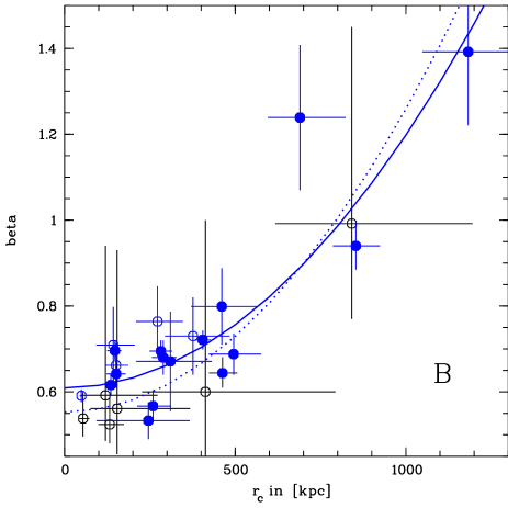
Figure 5: Same as Fig. 4 only that we now display the fit results of $\beta$–model B: isothermal $\beta$–model excising the central parts of the profile, if an improvement of reduced $\chi^{2}$ can be achieved (see Tab.1). Clusters belonging to the spectroscopic subsample are marked with filled circles.

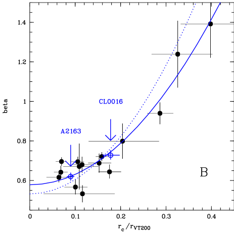
Figure 6: The correlation between scaled core radius $x_{\rm c}=r_{\rm c}/r_{\rm VT200}$ and $\beta$ for the 15 clusters of the spectroscopic subsample (see also Tab.1). The data points are for the $\beta$–model B and the error bars take into account the uncertainties in $r_{\rm VT200}$. Full line: $\beta$–$x_{\rm c}$ relation for $\beta$–model B. Dotted line: $\beta$–$x_{\rm c}$ relation for $\beta$–model A. We also display the results of A2163 located at $z=0.201$ (Arnaud et al. 1992; Elbaz, Arnaud & Böhringer 1995) and CL0016 at $z=0.54$ (Hughes & Birkinshaw 1998).

5.1 The $\beta$ and $r_{\rm c}$ values and the significance of the correlation

The slope parameter $\beta$ is not the same for all clusters, as would be the case for perfectly similar $\beta$–model density profiles. The $\beta$ values span a wide range, $0.47-1.04$ and $0.52-1.4$ for the $\beta$–model A and B, respectively. The distribution is not symmetric, it is clearly concentrated at low values, with rarer high values: the median value is $0.59$ for A (0.68 for B), $\sim 85\%$ of the values fall in the narrower range $0.47(0.52)-0.75$ and the standard deviation is only $0.14(0.21)$ or $24\%(30\%)$ of the median value for model A (model B). The same general features are observed for the core radius distribution. The median values are $143$ kpc and $278$ kpc for models A and B, respectively.

Fig. 4 displays the slope parameters $\beta$ against core radius $r_{\rm c}$, obtained with the $\beta$–model A. Fig. 5 is the equivalent plot for $\beta$–model B. A striking feature is that the data points are not distributed all over the $r_{\rm c}$–$\beta$ plane. There is a clear trend of increasing slope parameter with core radius, although the correlation is not very tight, specially at low core radius values. A quantitative measure of the correlation significance was obtained from three different tests, the Pearson’s test, the Spearman’s test, and the Kendall’s $\tau$ test (see Press et al. 1993). All three tests (applied to fit A results) give a high correlation significance, higher than 99.97%. The highest correlation significance is obtained with the Pearson’s test, with a value of $1.-2.99\times 10^{-10}$. The corresponding Pearson’s rank correlation is $r=0.902$.

5.2 The form of the $r_{\rm c}$–$\beta$ relation

The highest score obtained with the Pearson test indicates that the correlation between $r_{\rm c}$ and $\beta$ is close to being linear. One notes that the slope parameter is nearly constant at low core radii and starts to increase with $r_{\rm c}$ above $r_{\rm c}\sim 250$kpc only, which suggests a parabolic relation between the two quantities.

We examined which relation, linear or parabolic, better accounts for the data. For conciseness, the following discussion is based on a quantitative analysis of the parameters of the $\beta$–model A (similar results are obtained with $\beta$–model B).

We considered the two parametric functions

$$\beta=\beta_{\rm 0}^{l}\leavevmode\nobreak\ \left[1+\left(r_{\rm c}/r_{\rm s}^{l}\right)\right]$$ (10)

and

$$\beta=\beta_{\rm 0}\leavevmode\nobreak\ \left[1+\left(r_{\rm c}/r_{\rm s}\right)^{2}\right]$$ (11)

and fit them to the data. Since both quantities $\beta$ and $r_{\rm c}$ are marred with errors and the uncertainties are highly correlated, there is no well established method to define the best fit function parameters and to quantify the goodness of the fit. We used the following empirical least-squares method. Best fit parameters were derived by omitting the errors on $\beta$ and $r_{\rm c}$. The $\chi^{2}$ was minimised using the downhill simplex method (see Press et al. 1993). We got $\beta_{\rm 0}^{l}=0.49$ and $r_{\rm s}^{l}=870$ kpc for the linear function and $\beta_{\rm 0}=0.55$ and $r_{\rm s}=885$ kpc for the parabolic function (the corresponding curve is plotted on Fig.4). To compare the goodness of the fits obtained with the two functions we performed a subsequent $\chi^{2}$-test including the error on the $\beta$ quantity only. We utilised the $2-\sigma$ errors instead of the $1-\sigma$ errors. As the uncertainties of $\beta$ and $r_{\rm c}$ are correlated we assumed this could crudely take into account the two errors.

The reduced $\chi^{2}$ values for the entire cluster sample are 14.6 and 9.2 for the linear and parabolic function respectively. The fit is formally better for the parabolic relation but both $\chi^{2}$ are very high. If we exclude four clusters, A85, A780, A2319, and A3562, the reduced $\chi^{2}$ drops to 1.68 for the parabolic function. These four clusters lie offset of the correlation and have extremely small statistical error on $\beta$, less or equal to 2%. They boost therefore the $\chi^{2}$ value. The $\beta$-model parameters of these four clusters change significantly when one cuts out the central part (see Tab.1) and it is likely that using the global fit for these clusters is not a good approach. On the opposite we still obtain a reduced $\chi^{2}$ of 3.36 with the linear relation after the exclusion of the four principal outliers of this relation. Only when excluding seven clusters, we do obtain a reduced $\chi^{2}$ of 1.78, which is still higher than the $\chi^{2}$ of the parabolic fit, with four clusters excluded.

While keeping in mind that our criteria are not rigorous, we conclude that a parabolic relation between $r_{\rm c}$ and $\beta$ is a better description of the correlation between these two quantities than a linear relation. Henceforth, we will only consider a parabolic relation from now on.

5.3 The best fit $r_{\rm c}$–$\beta$ relation

Table 3: The best fit parameters of the $\beta$–core radius relations

Relation	$\beta$–model	normalisation	scale
$\beta$–$r_{\rm c}$	A	$\beta_{\rm 0}=0.55$	$r_{\rm s}=885$ kpc
$\beta$–$r_{\rm c}$	B	$\beta_{\rm 0}=0.61$	$r_{\rm s}=1020$ kpc
$\beta$–$x_{\rm c}$	A	$\beta_{\rm 0}^{\prime}=0.53$	$x_{\rm s}=0.27$
$\beta$–$x_{\rm c}$	B	$\beta_{\rm 0}^{\prime}=0.59$	$x_{\rm s}=0.34$

We determined the best fit parabolic relation $r_{\rm c}$–$\beta$ for both $\beta$–models A and B. The robustness of the $r_{\rm c}$–$\beta$ relation must be noted; it is not sensitive to the exact treatment of the central part of the cluster profile. From the $\beta$–model B data, plotted on Fig. 5, we got $\beta_{\rm 0}=0.61$ and $r_{\rm s}=1020$ kpc. These values are close to those obtained for the $\beta$–model A: $\beta_{\rm 0}$ is increased by only $\sim 10\%$ and $r_{\rm s}$ by $\sim 14\%$. The reduced $\chi^{2}$ is smaller: $\chi^{2}=1.92$ for the complete cluster sample; the $\chi^{2}$ drops to 1.42 if one excludes A780. Part of the improvement is certainly an artifact due to the larger uncertainties on $\beta$. The two relations look very much alike, as can be seen on Fig. 5.

As $\beta$ is a dimensionless quantity, while $r_{\rm c}$ is not, one would rather expect a relation between $\beta$ and a scaled core radius. Fig. 6 shows the correlation between $\beta$ and the scaled core radius $x_{\rm c}=r_{\rm c}/r_{\rm VT200}$, where the virial radius $r_{\rm VT200}$ is given by Eq.9 and the data points are from the $\beta$–model B. We fitted the parabolic relation

$$\beta=\beta_{\rm 0}^{\prime}\left[1+\left(x_{\rm c}/x_{\rm s}\right)^{2}\right]$$ (12)

to the cluster parameters of the 15 clusters in the spectroscopic subsample. We obtained $\beta_{\rm 0}^{\prime}=0.59$ and $x_{\rm s}=0.34$ for the $\beta$–model B and similar results $\beta_{\rm 0}^{\prime}=0.53$ and $x_{\rm s}=0.27$ for the $\beta$–model A (see also Tab.3).

An important question is whether $\beta$ is more tightly related to $r_{\rm c}$ or to $x_{\rm c}$. We cannot definitely answer this question with the present spectroscopic subsample. It is too small and covers a too narrow range in temperature and redshift. There is only a factor 2.4 between the minimum and maximum temperature. As $r_{\rm VT200}$ only scales as $\sqrt{T_{\rm X}}$, the effect of the scaling cannot be dramatic. However there are several indications that the ‘scaled’ relation is the most relevant one, as expected. First we compared Fig. 6 to Fig. 5 at large $\beta$ values ($\beta>0.65$), where the dependence of $\beta$ with $r_{\rm c}$ is maximal. For the clusters in the spectroscopic subsample (filled circles) the scatter around the best fit relation has been decreased by the scaling process. Second we considered test clusters outside the T and z range of our sample. A2163, the highest temperature cluster, fits well with both the $\beta$–$x_{\rm c}$ relation and the $\beta$–$r_{\rm c}$ relation, so this is not conclusive. On the other hand Cl0016+16, the most distant cluster with good estimates of $\beta$ and $r_{\rm c}$ ($\beta=0.728$, $r_{\rm c}=298$ kpc) fits much better with the $\beta$–$x_{\rm c}$ (see Fig. 6). This issue is further discussed in Sect. 6.

A summary of all fits of the $\beta$-$r_{\rm c}$ relation is given in Tab. 3. We do not give errors on the relation parameters, $\beta_{0}$ and $x_{\rm s}$ (or $r_{\rm s}$). We do not know of any proper method to estimate them since the uncertainties on the related quantities $\beta$ and $r_{\rm c}$ are highly correlated. We only suggest that they could be of the order of the difference observed when considering the two $\beta$–model A and B. We also want to stress that the relation parameters we determine here are in very good agreement with the direct study of the density profile shape presented below in Sect. 6.

Table 4: The $\beta$–$r_{\rm c}$ relation for various cluster samples

Number of	Choice	$\beta$–model	$\beta_{0}$	$r_{\rm s}$
clusters	criteria
26	none	A	$0.55$	$885$ kpc
26	none	B	$0.61$	$1020$ kpc
13	$r_{det}>1.45$Mpc	A	$0.54$	$859$ kpc
13	$\chi^{2}<1.6$	A	$0.56$	$980$ kpc
13	$r_{det}>1.45$Mpc	B	$0.60$	$1050$ kpc
15	$\chi^{2}<1.5$	B	$0.64$	$1080$ kpc

5.4 Checking on spurious effects

Could the derived correlation be an artifact of our data analysis? This question must be addressed since our results could in principle be affected by i) a choice of an inadequate model ii) the fitting process iii) systematic errors in the modeling of the instrument characteristics. We now discuss each point in turn.

5.4.1 The model

The $\beta$–model is only an approximation of the real gas density profile. Hence, the parameters derived may depend on the quality of the data and the cluster region used for the fit. We have already mentioned that a central excess can yield artificially low $\beta$ and core radii. At large radii the $\beta$–model tends to a simple power law. If instead the density profile continuously steepens, the $\beta$ value obtained from the fit will increase with the outermost radius used in the fit (see for instance the numerical simulations of Navarro, Frenk & White 1995) and as a result probably also the derived core radius. Moreover the magnitude of these effects will depend on the accuracy of the $\beta$–model approximation, which is likely to vary from cluster to cluster. All together this could induce a spurious correlation between the derived parameters, similar to the one observed,i.e. an apparent increase of $\beta$ with $r_{\rm c}$.

To see if this a serious issue we first investigated how the $\beta$–$r_{\rm c}$ relation is affected by the size of the region used for the fit. We can first compare $\beta$–models A and B. We also derived the relation for the half sample of the 13 clusters with the largest $r_{det}$, where $r_{det}$ is the maximum radius at which the X-ray emission is detected with a significance greater than $3\sigma$. Second we investigated if the relation is sensitive to the quality of the fit obtained with the $\beta$–model . For this purpose we selected the clusters with the lowest reduced $\chi^{2}$ and derived the corresponding $\beta$–$r_{\rm c}$ relation. The $\chi^{2}$ value is an indicator of the accuracy of the $\beta$–model approximation (but also depends on the quality of the data).

The parameters of the relations derived for the various cluster sub-samples are given in Tab. 4. In all cases, a parabolic $\beta$–$r_{\rm c}$ relation well accounts for the data. Furthermore for each model (A or B), the parameters $\beta_{\rm 0}$ and $r_{\rm s}$ depend very weakly on the selection on $r_{\rm det}$ ($0.3-3\%$ effect) or on the selection on the quality of the fit ($2-10\%$ effect). The largest discrepancy is actually seen between $\beta$–models A and B, i.e if one includes or not the central excess region in the fit. The effect is small as discussed in the previous section. From this observed robustness of the $\beta$–$r_{\rm c}$ relation we concluded that it is unlikely that it is an artifact due to the imperfection of the $\beta$–model .

5.4.2 The fitting process

To check the validity of the fitting procedure, we construct artificial clusters, which lie outside the correlation and have exposure times and countrates similar to the ones in our sample. We added Poisson noise to the images and treated these artificial clusters in the same way as our real data and fit the isothermal $\beta$-model to them. The intrinsic values for $\beta$ and $r_{\rm c}$ always lie well within the $2-\sigma$-errors of the fit results of the simulated clusters images. Thus, the fit procedure is correct and could not introduce a spurious correlation.

5.4.3 The instrument

As already discussed above, only two clusters could be affected by the finite instrument PSF, namely A780 and A1991. For the others, the PSF effects are of the same order than the statistical uncertainties or smaller. Excluding these two clusters from the fit changes the results of $\beta_{\rm 0}$ and $r_{\rm s}$ by less than $3\%$.

We also verified the exposure map calculation (or vignetting effects). We used the observations of clusters, that were not included in our sample because we found no prominent extended cluster emission. This is the case for A195 (observing title MKN 359) observed by the PSPC, and A1213 observed by the HRI (observing title 1113+29). For both pointings we divided the image of the actual data by the exposure map. There is no significant variation in the overall photon distribution when excluding obvious sources: the countrate is flat over the whole field of view of the corresponding detector. This also validates our implicit assumption of a flat background in the FOV.

6 The shape of the gas density profiles

A perfect similarity between the density profiles is ruled out by the variation of $\beta$ from cluster to cluster. On the other hand the correlation found between the two shape parameters of the density profile indicates some structural regularity in the gas distribution, that we study in this section. For that purpose we use the density profiles derived from our $\beta$–model fits of the observed brightness surface profiles.

6.1 Quantifying the shape: the slope profile

The shape of the gas density distribution may be quantified by the variation with radius of its logarithmic derivative. This derivative is also important for the estimate of the mass profiles (see Sect. 7). For the $\beta$–model form, it reads:

$$\alpha_{\rm n}(r)=-\frac{d\log n_{\rm g}(r)}{d\log r}=\frac{3\leavevmode\nobreak\ \beta}{\left[1+\left(r_{\rm c}/r\right)^{2}\right]}$$ (13)

or equivalently, in term of the scaled radial coordinates:

$$\alpha_{\rm n}(x)=\frac{3\leavevmode\nobreak\ \beta}{\left[1+\left(x_{\rm c}/x\right)^{2}\right]}$$ (14)

We will refer to this function as the slope profile: $\alpha_{\rm n}(r)$ is the slope of the gas distribution in the log–log plane at radius $r$. It depends on the two shape parameters of the $\beta$–model : the core radius and $\beta$.

6.2 The slope profiles for a theoretical parabolic $\beta$ - core radius relation

For a parabolic relation between $\beta$ and $r_{\rm c}$ (Eq. 11), the slope profile may be written as:

$$\alpha_{\rm n}(r)=3\leavevmode\nobreak\ \beta_{\rm 0}\leavevmode\nobreak\ \frac{\left[1+\left(r_{\rm c}/r_{\rm s}\right)^{2}\right]}{\left[1+\left(r_{\rm c}/r\right)^{2}\right]}$$ (15)

Similarly for a parabolic relation between $\beta$ and the scaled core radius:

$$\alpha_{\rm n}(x)=3\leavevmode\nobreak\ \beta_{\rm 0}^{\prime}\leavevmode\nobreak\ \frac{\left[1+\left(x_{\rm c}/x_{\rm s}\right)^{2}\right]}{\left[1+\left(x_{\rm c}/x\right)^{2}\right]}$$ (16)

The physical implications of the parabolic relation, is straightforward from these two equations: i) if $\beta$ is related to $r_{\rm c}$, there is a specific radius, $r_{\rm s}$, where the slope of the gas density profile is the same for all clusters, ii) if $\beta$ is instead related to the scaled core radius, this occurs at a specific scaled radius, $x_{\rm s}$.

Let us first assume a relation between $\beta$ and $r_{\rm c}$. At the specific radius $r_{\rm s}$ the slope is equal to $3\leavevmode\nobreak\ \beta_{\rm 0}$, where $\beta_{\rm 0}$ is the normalisation factor of the parabolic relation. At very large radii, $r\leavevmode\nobreak\ >>\leavevmode\nobreak\ r_{\rm c}$, $\alpha_{\rm n}(r)$ tends to $3\leavevmode\nobreak\ \beta$ - the $\beta$–model is equivalent to a power law - and there is no impact of the $\beta$–$r_{\rm c}$ relation. At low radii, $\alpha_{\rm n}(r)$ roughly scales as $\left(r_{\rm c}/r\right)^{2}$ and in view of the large dynamical range of core radii values, it can vary by more than an order of magnitude from cluster to cluster. This is illustrated on Fig. 7 where we have plotted with thick lines two extreme slope profiles corresponding to the best fit $\beta$–$r_{\rm c}$ parabolic relation derived in Sect. 5.3 (Eq. 15 with parameters from Tab. 3). The first one, $\alpha_{\rm n}^{(1)}(r)$, corresponds to the minimum allowed $\beta$ value: $\beta=\beta_{\rm 0}$ or $r_{\rm c}=0$. In that case $\alpha_{\rm n}(r)$ keeps constant with radius: $\alpha_{\rm n}^{(1)}(r)=3\leavevmode\nobreak\ \beta_{\rm 0}$. The second one, $\alpha_{n}^{(2)}(r)$, corresponds to the maximum $\beta$ value observed in our sample. The two curves cross at $r_{\rm s}$.

The same properties hold for the $\beta$–$x_{\rm c}$ relation, in terms of the scaled radial coordinates.

6.3 The observed slope profiles

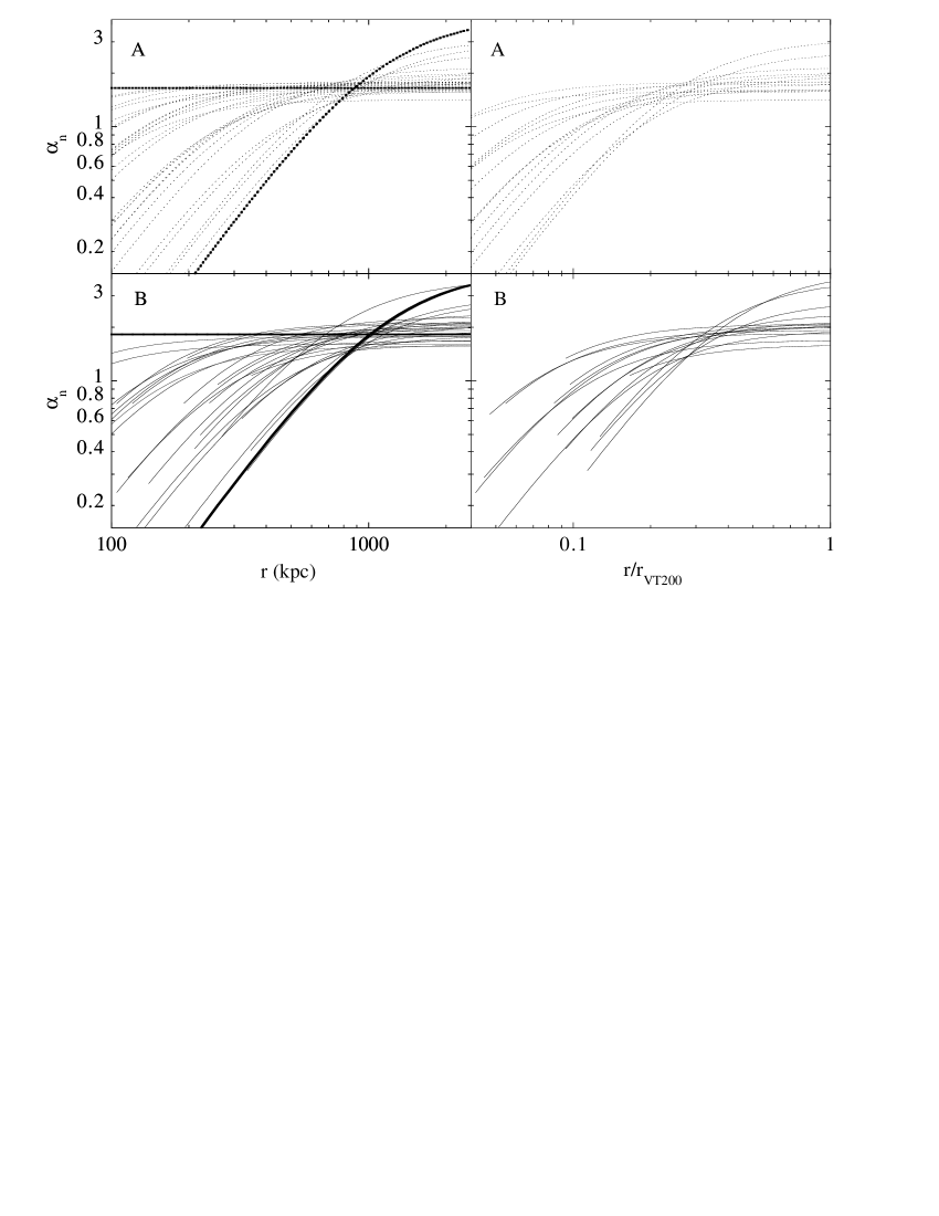
Figure 7: The variation with radius of the logarithmic slope of the gas density distribution. Top-left panel: the slope profiles $\alpha_{\rm n}(r)=-d\log(n_{\rm g}(r)/d\log r$ versus radius $r$ derived from the best-fit $\beta$–model A, for all clusters of the sample. The bold lines correspond to the extreme slope variations allowed by the $\beta$–$r_{\rm c}$ correlation (Eq.11 with parameters from Tab. 3 and Eq.15): the horizontal line is for $\beta=\beta_{0}=0.55$, $r_{\rm c}=0$ and the other line is for $\beta=1.4$, $r_{\rm c}=1100$ kpc. Top-right panel: the slope profiles $\alpha_{\rm n}(x)=-d\log(n_{g}(x)/d\log x$ versus scaled radius $x=r/r_{\rm VT200}$ for the spectroscopic subsample ($\beta$–model A). Bottom panels: Same as top panels but for $\beta$–model B. In that case the profiles are plotted only beyond the excised central region.

Figure 8: Structural variations within the cluster sample. The average of $\alpha_{\rm n}$ (top panels) and its relative dispersion (bottom panels) are plotted as a function of radius (left) for the whole sample and scaled radius (right) for the spectroscopic subsample. The relative dispersion is defined as spread normalised to the average value. Thick lines: bi-weight estimators. Thin lines: classical estimators. Dotted lines: results for $\beta$–model A. Full lines: results for $\beta$–model B. Arrows in left-top panel: They indicate the bi-weight mean values of the core radii $r_{\rm c,A}$ and $r_{\rm c,B}$ for $\beta$–model A and B respectively; the bi-weight mean $R_{\rm cut}$; the specific radius $r_{\rm s,A}(r_{\rm s,B})$ of the $\beta$–$r_{\rm c}$ correlation for $\beta$–model A(B). Arrows in right-top panel: Same for scaled coordinates. Dashed line in top-right panel: slope profile obtained for $\beta=0.67$, $x_{\rm c}=0.13$.

The slope profiles $\alpha_{\rm n}(r)$ derived from model A and B are plotted on the left panels of Fig. 7 for all clusters in our sample. On the right panels are plotted the profiles $\alpha_{\rm n}(x)$ against scaled radius for the spectroscopic subsample.

To quantify structural variations within the cluster sample, we estimated at each radius, the center and spread of the distribution of slopes at that radius. We used both the classical estimators (mean value and standard deviation) and the bi-weight estimators (bi-weight location and scale). The latter are more resistant and robust than the former (Beers, Flynn & Gebhardt 1990). The results are shown in Fig. 8. The “average” slope (top panels) and the “relative dispersion around the mean”, defined as the spread normalised to the average value (bottom panels) are plotted as a function of radius (left) for the whole sample and scaled radius (right) for the spectroscopic subsample. The results of model A (dotted lines) and model B (full lines) are provided. We also computed the bi-weight means of the core radii and cut-out radii $R_{cut}$, the locations of which are indicated by arrows in the figure.

6.4 General properties

The characteristics of the observed profiles are those expected from the best fit $\beta$–core radius relations we derived. Let us consider for instance the slope profiles $\alpha_{\rm n}(r)$ derived from model B. At small radii the observed profiles lie well within the two extreme curves $\alpha_{\rm n}^{(1)}(r)$ and $\alpha_{\rm n}^{(2)}(r)$ corresponding to the best fit $\beta$–$r_{\rm c}$ relation and the scatter is very large among the cluster population (Fig. 7, bottom-left panel). This scatter diminishes with radius until it reaches a minimum at the specific radius $r_{\rm s}=1020$ kpc (Fig. 7 and Fig. 8 bottom-left panel). At that radius the average $\alpha_{\rm n}$ value agrees well with the best fit $3\leavevmode\nobreak\ \beta_{\rm 0}$ value (Fig. 8 top–left panel). The classical and bi-weight estimators give the same results, the slope distribution at that radius being close to Gaussian. The residual scatter on $\alpha_{\rm n}$ at $r_{\rm s}$ - the slope is not exactly the same for all clusters - can naturally be explained by the scatter around the best fit $\beta$–$r_{\rm c}$ relation. Above $r_{\rm s}$ the scatter increases again, but saturate at a value of the same order as the variations of $3\leavevmode\nobreak\ \beta$, the asymptotic value of the slope. For instance, at 2.5 Mpc the bi-weight mean slope is 1.96 and the bi-weight relative spread is 17%, very close to the corresponding values for $3\leavevmode\nobreak\ \beta$: 1.98 and 18% respectively. At these large radii the bi-weight mean and dispersion are smaller than the classical estimators, reflecting the non-Gaussian $\beta$ distribution which presents a tail at high values (see Sect 5.1).

These general properties hold both for $\beta$–model A and B. They do not depend on the choice of the radial coordinates (physical or scaled radius). However, there are some quantitative differences between the corresponding data sets.

The relative dispersion of the slope $\alpha_{\rm n}(r)$ is higher for the $\beta$–model B than for the $\beta$–model A at all radii. This may result in part from the larger uncertainties on $\beta$ and $r_{\rm c}$, which introduce extra scatter. Using the scaled radii instead (Fig. 8 bottom-right panel), the relative dispersion of $\alpha_{\rm n}$ for $\beta$–model B decreases. The minimum dispersion, about 9%, is similar for A and B in this case. This further supports the idea that it is better to work with scaled coordinates, in agreement with the results of Sect.5.3. Furthermore the bi-weight dispersion for model B now becomes slightly smaller than the dispersion for the model A, beyond the region where the dispersion is minimal ($x\sim 0.3$). This is more satisfactory since the model B should be a better fit to the data at large radii as model A is expected to introduce extra scatter. From now on we will only work in scaled coordinates.

The mean slope value is smaller at low radii (the density distribution is flatter on average) and higher at high radii (steeper density distribution) for the $\beta$–model B than for the $\beta$–model A (Fig. 8 top panels). This is a direct consequence of the treatment of a possible central excess, as explained in details in Sect. 4. This central excess typically occurs within $x_{cut}=0.08$, the bi-weight mean cut-out radius. Beyond $r/r_{\rm VT200}\sim 0.1$ the systematic difference between the two models becomes smaller than the intrinsic dispersion observed within the cluster population. The mean slopes for model A and B became identical in the region of minimum dispersion ($x\sim 0.3$). This is consistent with the robustness of the $\beta$–$x_{\rm c}$ relation already noted (Sect.5.3). This means that the determination of the mean slope around that scaled radius is very robust and does not depend on the exact model used to fit the data.

The mean slope profile can be approximated within a few percent with the profile corresponding to the bi-weight mean core radius $\bar{x_{\rm c}}=0.13$ and $\beta$ value $\bar{\beta}=0.67$ (see Fig. 8 top-right panel).

6.5 The standard density profile and structural variations in the cluster population

In view of the shape characteristics of the observed density profiles, it is natural to define a standard profile: this density profile follows a $\beta$–model in scaled coordinates with $x_{\rm c}=0.13$ and $\beta=0.67$. We recall that the cluster physical radius scales as $T_{\rm X}^{1/2}$.

The typical deviations from this standard profile are the following:

• A central excess compared to the $\beta$–model can be observed in the central part, typically within $x_{\rm cut}=0.08$. In that region the scatter in density profile shape is very large (more than $100\%$ variation in logarithmic slope) among the cluster population.

• Beyond $x=0.2$ the bi-weight dispersion of the observed slopes $\alpha_{\rm n}(x)$ becomes less than $20\%$ of the slope of the standard $\beta$–model profile.

• The dispersion is minimal at $x=0.3$ where $\alpha_{\rm n}(x)=1.67\pm 0.18$. This corresponds to the observed correlation between core radius and $\beta$ values.

Note that these values are derived from our spectroscopic-subsample (Fig. 8), which concerns relatively hot clusters. Cooler clusters may present larger variations.

7 Consequences for the total mass profile and the $M$–$T$ relation

X-ray astronomers usually utilize the hydrostatic approach to calculate the total mass of a cluster within a certain radius :

$$M_{\rm tot}(r)=-\frac{{\rm k}T}{\rm G\mu m_{p}}r\left(\frac{d\log n_{\rm g}(r)}{d\log r}+\frac{d\log T}{d\log r}\right)$$ (17)

Figure 9: The normalised mass profiles of the 15 clusters in the spectroscopic subsample. For each cluster the mass is derived from the hydrostatic equation and our best fit isothermal $\beta$–model (Dotted line: $\beta$–model A; Full line: $\beta$–model B). The mass is normalised to $M_{\rm VT200}$, the mass at density contrast 200 derived from the numerical simulations of EMN96. The bold line is the profile derived by these authors.

If the ICM is isothermal or if the temperature gradient can be neglected in front of the density gradient, one may express the total mass as a function of the X-ray temperature and the gas density logarithmic slope $\alpha_{\rm n}$. Using the scaled radial coordinates one gets:

$$M_{\rm tot}(x)=4.13\times 10^{15}\left(\frac{T_{\rm X}}{10\leavevmode\nobreak\ \mbox{keV}}\right)^{3/2}\frac{x\leavevmode\nobreak\ \alpha_{\rm n}(x)}{(1+z)^{3/2}}\leavevmode\nobreak\ {\rm M_{\odot}}$$ (18)

where $\alpha_{\rm n}(x)$ is given by Eq. 14 for a $\beta$–model .

It is convenient to normalize the mass profile to the virial mass at density contrast 200 derived from numerical simulation (Evrard, Metzler & Navarro 1996):

$$M_{\rm VT200}=2.92\times 10^{15}\leavevmode\nobreak\ \left(\frac{T_{\rm X}}{10\leavevmode\nobreak\ \mbox{keV}}\right)^{3/2}(1+z)^{-3/2}\leavevmode\nobreak\ {\rm M_{\odot}}$$ (19)

The corresponding scaled total mass profile, $\widetilde{M_{\rm tot}(x)}$, is directly related to the variation of the gas density slope $\alpha_{\rm n}(x)$:

$$\widetilde{M_{\rm tot}(x)}=\frac{M_{\rm tot}(x)}{M_{\rm VT200}}=0.472\leavevmode\nobreak\ x\leavevmode\nobreak\ \alpha_{\rm n}(x)$$ (20)

Fig. 9 shows the total mass profiles, $\widetilde{M_{\rm tot}(x)}$, derived from our best fit $\beta$–model A (dotted lines) and B (full lines), for all the clusters of the spectroscopic subsample. As for $\alpha_{\rm n}(x)$, the differences between the two models are smaller than the dispersion in the cluster population.

The scatter in the total mass profiles is the same as for $\alpha_{\rm n}(x)$ and is minimal at about $x_{\rm s}=0.3$, the specific radius of the $\beta$–core radius relation. At that scaled radius $\alpha_{\rm n}(x_{\rm s})=1.67\pm 0.18$ and $\widetilde{M_{\rm tot}(x_{\rm s})}=0.236\pm 0.025$. In physical coordinates this corresponds to:

$$r_{\rm s} = \frac{1.11}{(1+z)^{3/2}}\leavevmode\nobreak\ \left(\frac{T_{\rm X}}{10\leavevmode\nobreak\ \mbox{keV}}\right)^{1/2}\leavevmode\nobreak\ \mbox{Mpc}$$ (21)

$$M_{\rm tot}(r_{\rm s}) = \frac{(6.90\pm 0.74)\times 10^{14}}{(1+z)^{3/2}}\left(\frac{T_{\rm X}}{10\leavevmode\nobreak\ \mbox{keV}}\right)^{3/2}{\rm M_{\odot}}$$ (22)

Note that the numerical values in these equations do not depend of the calibration of $r_{\rm VT200}$ and $M_{\rm VT200}$. The radius of minimal dispersion corresponds to a density contrast of $\delta=1750$ (for the mass computed from the isothermal $\beta$–model ).

The mean mass profile, corresponding to $x_{\rm c}=0.13$ and $\beta=0.67$, and the two curves corresponding to this mean plus or minus the bi-weight dispersion are plotted on Fig 10. For comparison we also plotted the mass profile derived from the numerical simulations of Evrard, Metzler & Navarro (1996; hereafter EMN96; Table 5). The isothermal $\beta$–model yields lower values but the discrepancy decreases with radius and is less than $10\%$ around $x=1$. Both models would give equal values at $x=1$ for $\beta\sim\alpha_{\rm n}(1)/3=0.71$ (from Eq. 20), whereas the mean $\beta$ value is only $6\%$ lower.

Figure 10: Comparison between mass estimates for the spectroscopic subsample. Bold line: Numerical simulations of EMN96. Full lines: The middle curve is the mean mass profile for our sample derived from the isothermal $\beta$–model ($x_{\rm c}=0.13$ and $\beta=0.67$); The top and bottom curves correspond to this mean plus or minus the bi-weight dispersion. Dotted line: The mean mass profile for the same $\beta$–model but with a polytropic temperature profile of index $\gamma=1.2$, approximating the results of Markevitch et al. (1998).

The isothermal assumption may give poor estimates of the total mass if strong temperature gradients are present. Recent observations with ASCA suggest that the temperature does decrease with radius, although the uncertainties on the temperature profiles are still large (Markevitch et al. 1998). To illustrate the impact of such a temperature gradient we considered the composite projected temperature profile derived by Markevitch et al. (1998, Figure 7) from a sample of bright clusters. This profile is steeper than most of the profiles derived from available simulations (Markevitch et al. 1998) and thus is likely to give an upper limit on the influence of a temperature gradient, at least up to $x=0.5$ the limit of the observations. We found that the shape of the projected temperature profile, $\bar{T}(x)$, can be well approximated by a polytropic model with an index of $\gamma=1.25$, a normalisation factor $A=1.2$ and our mean $\beta$–model density profile ($\beta=0.67$, $x_{\rm c}=0.13$):

$$\frac{\bar{T}(x)}{T_{\rm X}}=A\left(\frac{n_{\rm g}}{n_{\rm g0}}\right)^{\gamma-1}=A\left[1+\left(x/x_{\rm c}\right)^{2}\right]^{-\frac{3\beta}{2}\left(\gamma-1\right)}$$ (23)

Assuming that the observed temperatures correspond to the emission weighted mean temperatures along the line-of-sight, it is easy to show that the radial temperature profile, $T(x)$, also obeys the same polytropic law with a higher normalisation factor, about $10\%$ higher for the parameters we derived.

For a polytropic gas, the temperature logarithmic slope $\alpha_{\rm T}$, entering the hydrostatic equation (Eq. 17), is simply related to the corresponding density slope:

$$\alpha_{\rm T}(x)=(\gamma-1)\leavevmode\nobreak\ \alpha_{\rm n}(x)$$ (24)

The corresponding mass profile, plotted on Fig. 10, is thus:

$$\widetilde{M_{\rm tot}(x)}=0.472\leavevmode\nobreak\ \gamma\frac{T(x)}{T_{\rm X}}\leavevmode\nobreak\ x\leavevmode\nobreak\ \alpha_{\rm n}(x)$$ (25)

The mass is larger than the isothermal estimate below $x\sim 0.35$ and higher above. At $x=0.3$ the correction is only $4\%$, less than the typical scatter. At large radii the differences are drastic: at $x=1$ the isothermal estimate is 1.7 times higher than the estimate using the polytropic model. Whereas in the isothermal case we deduce a mass profile shallower than found in numerical simulation (EMN96), the mass profile is now slightly more peaked than the theoretical one. We must however emphasize that the temperature profile used is based on an extrapolation of the data beyond $x=0.5$.

8 Discussion and Conclusions

We have studied the shape of the surface brightness profiles of a sample of clusters covering a large variety of morphological types. The surface brightness distribution in the ROSAT band hardly depends on temperature and can be directly translated into the gas density distribution. Although the gas density profiles of the clusters are not perfectly similar, our quantitative analysis gives evidence for structural regularity:

• We found converging evidence that there is a scaling radius in clusters which varies as $T^{1/2}$. The surface brightness profiles appear more similar once the physical radii are scaled. The $\beta$–core radius relation is tightened and the scatter of the density profile slopes is reduced. However the small range in temperature and redshift of our sample precludes any definitive conclusion, in particular on the exact variation of the scale radius with $T$.

• There is a parabolic correlation between the two shape parameters of the $\beta$–model : the core radius and the slope. Cluster density profiles essentially constitute a one shape parameter family.

• We observe a very large scatter of the surface brightness profiles in the central part of clusters. A central excess compared to the $\beta$–model can be present, typically within $x_{\rm cut}=0.08$. In this region the logarithmic slope can vary by more than a factor of $2$ and the emission measures at the center are spread over two orders of magnitude.

• Beyond a scaled radius of $x=0.2$, the density profiles are remarkably similar in shape and resemble a $\beta$–model profile with a core radius of $x_{\rm c}=0.13$ and $\beta=0.67$. The bi-weight dispersion of the logarithmic slope $\alpha_{\rm n}(x)$ at a given radius is less than $20\%$. At the virial radius the logarithmic slope is close to $3\beta$. Its distribution reflects the distribution of this parameter, which has a bi-weight dispersion of only $18\%$ but presents a tail of rare high values. The scatter is minimal at $x=0.3$ where $\alpha_{\rm n}(x)=1.67\pm 0.18$ with a gaussian distribution. This minimum is related to the correlation between $x_{\rm c}$ and $\beta$. These results at $x=0.3$ are insensitive to the exact treatment of a possible central excess when fitting the profiles.

As the gas evolves in the potential of the dark matter it is unlikely that such regularity in the gas density profile shape can be observed without a comparable regularity in the dark matter profiles. Similarity of the dark matter profiles is naturally expected in hierarchical clustering scenario (Teyssier, Chièze & Alimi 1997; Navarro, Frenk & White, 1997) and our results therefore give support to it. However, the gas density is not the sole tracer of the gravitational potential. If a universal profile for the dark matter is responsible for the similarity of the X-ray profiles, one also expects that the temperature profiles have similar shapes. Both numerical simulations (e.g. Navarro, Frenk & White 1995; EMN96) and recent X-ray observations (Markevitch et al. 1998) indicate that this is probably the case.

Our results are consistent with a scaling radius which goes as $T^{1/2}$ as expected if clusters form at constant overdensity. However our sample is too small to exclude other scaling laws as, for instance, the slight variation of overdensity with mass obtained by Navarro, Frenk & White (1997).

Similarity breaking in the X-ray properties of clusters is expected if non adiabatic processes play an important role in the evolution of the gas. These include radiative cooling and possible heating by galactic winds.

Radiative cooling is known to be more important in the cluster core where the cooling time, which scales as the gas density, is shorter. The presence of Cooling Flows of various strengths most probably explains the variation we observe in the density profiles below $x=0.1$. The large scatter could be either due to intrinsic variation in the initial gas density in the core, and thus in the cooling time, or to variation in the Cooling Flow “age”. The first explanation is unlikely in view of the observed quasi-similarity of the scaled emission measure profiles at large radii. Let consider perfectly similar clusters obeying the assumptions used in the scaling of the profiles. The mean density of clusters in a given redshift range is a constant (formation at fixed overdensity) and since the gas mass fraction does not vary from cluster to cluster, the mean gas density is also a constant. As the density profiles are similar in shape, the central density is also constant and so is the cooling time. No major break of similarity in the core compared to external regions is thus expected, if clusters have the same “age”. The very large scatter observed in the core properties thus favors a scenario where Cooling Flows are recurrent phenomena that are periodically erased by strong mergers, a natural feature of hierarchical clustering (Fabian et al. 1994). In that case the observed variety of core properties in the cluster population would naturally reflect the statistics of the formation process via merger events.

Non gravitational heating, such as extra energy inputs by galactic winds, is thought to play an important role in the ICM physics. In ”pre-heating” scenarios, early winds add roughly a constant entropy to the system and thus affect cooler clusters more strongly, hence breaking the similarity law. The main expected effect of these winds is to inflate the gas distribution. Preheating scenarios can thus explain the observed steepening of the $L_{\rm X}$–$T$ and size-temperature relations relative to the similarity scaling (Arnaud & Evrard 1998, Mohr & Evrard 1997, Cavaliere, Menci & Tozzi 1998). Further support to this scenario was recently given by Ponman, Cannon & Navarro (1998) who showed that the entropy of cool systems is indeed higher than what can be achieved through gravity alone. They consistently put into evidence similarity breaking in the surface brightness profiles of clusters: cooler clusters have systematically shallower profiles than hotter systems. The regularity we found in the gas density profiles beyond the core does not contradict such results. Our spectroscopic subsample comprises relatively hot clusters. Our quantitative study simply shows that non gravitational heating is negligible above k$T\sim 3.5\leavevmode\nobreak\ {\rm keV}$. This is in agreement with the quantitative deviations from similarity laws observed in clusters. The gas entropy at $x=0.1$ plotted by Ponman, Cannon & Navarro (1998) as a function of cluster temperature levels off from the similarity law only below $\sim 3$ keV. Similarly the variation of the structure parameter $\hat{Q}(T)=\langle{n_{gas}^{2}}\rangle/\langle{n_{gas}}\rangle^{2}$, which characterises the concentration of the gas distribution and plays a role in the steepening of the $L_{\rm X}$–$T$ relation, has been studied by Arnaud & Evrard (1998, Figure 2). An increase with temperature has been noted but the effect is again stronger below $4$ keV. The existence of such a ”threshold” around $3-4$ keV clearly favors scenarios with constant entropy inputs. In turn it shows that the outer regions of hot clusters are good tracers of purely gravitational processes.

The mean gas density profile we derived is shallower than found in CDM simulations without winds. For instance Navarro, Frenk & White (1995, Table 2) found a mean core radius $x_{\rm c}=0.10$ and a mean $\beta$ of $0.82$, while Eke, Navarro & Frenk (1998, Table 3) derived for a low $\Omega$ Universe average values of $x_{\rm c}=0.05$ and $\beta=0.73$. If pre-heating is negligible in our spectroscopic subsample other effects can explain the difference. First the transfer of entropy from the dark matter to the gas, which has been invoked to explain the segregation between these two components (Eke, Navarro & Frenk 1998; see also Teyssier, Chièze & Alimi 1997), may be larger than predicted in the simulation. We can also speculate that the dark matter distribution itself is actually less concentrated, as, for instance, expected if some hot dark matter is present (see also below).

The gas structural variations throughout the cluster population are small beyond $x=0.2$ but depend on the radius considered. The logarithmic slope $\alpha_{\rm n}(x)$ of the density profile presents a minimum spread at $x\sim 0.3$. This scatter then increases with radius and some clusters present large asymptotic slopes compared to the mean asymptotic slope. The $\beta$–model , used in our study, is reasonably accurate to estimate both the gas density distribution and total mass distribution, as shown by the hydrodynamic simulations of Schindler (1996) or EMN96. However, by fitting such a model to simulated galaxy clusters, these last authors found that it introduces an extra-scatter in the total mass estimate and that this scatter increases with radius. We probably see the same effect here. In the hydrostatic isothermal $\beta$–model , the logarithmic slope of the density profile is directly linked to the total mass. For a given dark matter profile, scatter in the gas density slope estimate can be introduced by i) errors in the measure due to the background determination and statistical errors; ii) departure from a spherically symmetric $\beta$–model for the gas distribution due to imperfection of the model, bimodality, ancient mergers, and high eccentricities; iii) departure from the hydrostatic equilibrium. The first and third effects are expected to be larger in the outer regions. On the contrary, the signal to noise is very high in the region around $x=0.3$ and the gas density slope, which is the derivative of the profile at that radius, is tightly constrained. This probably explains why the scatter in the slope estimate is minimum there and why the derived slope value is insensitive to the exact model used to fit the data (model A or B). In conclusion the observed variation of the scatter with radius is more likely an artifact due to the modeling of the data, rather than the direct consequence of similar variations in the dark matter profiles.

The slope at $x\sim 0.3$ is almost the same for all clusters. Since, in the $\beta$–model , it depends on both $\beta$ and core radius, the values of these two parameters are correlated throughout the cluster population, as we did observe. This very correlation between $\beta$, that controls the outer slope, and $x_{c}$, that controls the core size, may indicate that the best model to fit the data is not the two parameter $\beta$–model but some other model, involving only one shape parameter (scaling with the virial radius).

As a result of the small scatter on $\alpha_{\rm n}(x)$, the spread in the scaled mass profiles derived from the hydrostatic isothermal $\beta$–model is small. The uncertainty on the dark mass profile, deduced from the hydrostatic equation, is dominated by the systematic uncertainty on the temperature gradients, rather than by the intrinsic scatter in the gas density profiles.

The radius at which the scatter of the gas logarithmic slope is lowest is most likely in the region in which the $\beta$–model gives the most accurate result on the total mass of clusters. It is also in the region in which temperature gradients are not expected to play a large role, as indicated both by numerical simulations (e.g. EMN96) and by the observed temperature profiles (see previous section). We thus propose the $M$–$T$ ($r$–$T$) relation, we derived at $x=0.3$ (Eq. 22) from the hydrostatic isothermal $\beta$–model , as a reference test point for numerical simulations.

In this relation the mass scales classically as $T^{3/2}\leavevmode\nobreak\ (1+z)^{-3/2}$. The normalisation at $x=0.3$ is however $\sim 30\%$ lower than found in the numerical simulations of EMN96, whereas these authors did not observe any significant bias at that radius in the isothermal $\beta$–model estimate. One can speculate again that the dark matter profile is in fact shallower than in CDM simulations, as expected if some HDM is present. However the discrepancy could also indicate that the temperature spatial variations or bulk motions and residual velocity dispersion of the gas are higher than expected. In that case the hydrostatic isothermal equation underestimates the real mass. Large velocity fields are naturally associated with recent formation or accretion. Therefore their properties should strongly depend on the specific history of each individual cluster and the corresponding velocity profiles are expected to present a high relative scatter. If large kinetic energy is common in the cluster population, it would thus be surprising that the gas density profiles remain similar. In conclusion we think that the regularity of the gas density profiles supports the validity of the hydrostatic equation. On the other hand quasi-similar temperature profiles corresponding to large temperature gradients could well be present. It thus is essential to accurately measure the temperature profiles of large sample of clusters to establish firmly the normalisation of the $M$–$T$ relation and the shape of the dark matter profile. This will be soon possible with XMM and AXAF.

- (1) Abell G.O., Corwin H.G. Jr., Olowin R.P., 1989, ApJS, 70, 1
- (2) Allen S.W., Fabian A.C., 1998, MNRAS, 297, L57
- (3) Arnaud M., Hughes J.P., Forman W., Jones C., Lachièze-Rey M., Yamashita K., Hatsukade I., 1992, ApJ, 290, 345
- (4) Arnaud M., Evrard A.E., 1998, MNRAS, astro-ph/9806353
- (5) Beers T., Flynn K ., Gebhardt K., 1990, AJ, 100, 32
- (6) Cavaliere A., Menci N., Tozzi P., 1998, MNRAS, astro-ph/9810498
- (7) David L.P., Slyz A., Jones C., Forman W., Vrtilek S.D., Arnaud K.A., 1993, ApJ, 412, 479.
- (8) Ebeling H., Voges W., Böhringer H., Edge A.C., Huchra J.P., Briel J.G., 1996, MNRAS, 281, 799
- (9) Eke V.R., Navarro J.F., Frenk C.S., 1998, ApJ, 563, 569
- (10) Elbaz D., Arnaud M., Böhringer H., 1995, A&A, 293, 337
- (11) Evrard A.E., Metzler C.A., Navarro J.F., 1996, ApJ, 469, 494
- (12) Evrard A.E., MNRAS, 1997, 292, 289
- (13) Fabian A.C., Crawford C.S., Edge A.C., Mushotzky R.F., 1994, MNRAS, 267, 779
- (14) Henriksen M.J., Markevitch M., 1996, ApJ, 466L, 79
- (15) Hughes J., Birkinshaw, M., 1998, ApJ, 501, 1
- (16) Hjorth J., Oukbir J., van Kampen E. 1998, MNRAS, 298, L1
- (17) Jones C., Forman, W., 1984, ApJ, 276, 38
- (18) Makino N., Sasaki S., Suto Y., 1998, ApJ, 497, 555
- (19) Markevitch M., 1998, ApJ , 504, 27
- (20) Markevitch M., Forman W., Sarazin C., Vikhlinin A., 1998, ApJ , 503, 77
- (21) Mohr J.J., Evrard A.E., 1997, ApJ, 491, 38
- (22) Navarro J.F., Frenk C.S., White S.D.M., 1995, MNRAS, 275, 720
- (23) Navarro J.F., Frenk C.S., White S.D.M., 1996, ApJ, 462, 563
- (24) Navarro J.F., Frenk C.S., White S.D.M., 1997, ApJ, 490, 493
- (25) Ponman T.J., Cannon D.B., Navarro J.F., Nature in press astro-ph/9810359
- (26) Press W.H., Teukolsky S.A., Vetterling W.T., Flannery B.P., 1993, Numerical Recipes in C : The Art of Scientific Computing, Cambridge University Press
- (27) Roettiger K., Stone J.M., Mushotzky R.F., 1998, ApJ, 493, 62
- (28) Schindler S., 1996, A&A, 305, 756
- (29) Snowden S., 1998, ApJ, in press
- (30) Teyssier R., Chieze J.P., Alimi J.M., 1997, ApJ, 480, 36
- (31) White, D., Jones C., Forman W., 1997, MNRAS, 292, 419
- (32) Zabludoff A.I., Zaritsky D., 1995, ApJ, 447L, 21