Probing the BLR in AGNs using time variability of associated absorption lines

Abstract

It is know that most of the clouds producing associated absorption in the spectra of AGNs and quasars do not completely cover the background source (continuum + broad emission line region, BLR). We note that the covering factor derived for the absorption is the fraction of photons occulted by the absorbing clouds, and is not necessarily the same as the fractional area covered. We show that the variability in absorption lines can be produced by the changes in the covering factor caused by the variation in the continuum and the finite light travel time across the BLR. We discuss how such a variability can be distinguished from the variability caused by other effects and how one can use the variability in the covering factor to probe the BLR.

1 Introduction

It is known that roughly 10$\%$ of the high redshift QSOs show associated absorption lines, (i.e systems with absorption redshift, $z_{\rm abs}$, greater than or equal to the emission redshift, $z_{\rm em}$ ) super-imposed on the broad emission lines (Weymann et al., 1979; Foltz et al., 1986; Sargent, Boksenberg & Steidel, 1988; Barthel et al. 1991). It is believed that these absorption systems could be due to gas intrinsically associated with the central engine of the QSO and/or with the ambient medium surrounding the QSO (for example interstellar medium of the galaxies in the cluster in which QSO is also a member). Heavy element abundance studies, using broad emission lines and associated absorption systems in QSOs, suggest that the QSOs are the sights of vigorous star formation activity at very early epochs (Hamann & Ferland, 1993; Petitjean et al., 1994; Hamann, 1997).

IUE observations suggested only 3$\%$ of the the low $z$, low luminosity, AGNs (Seyferts) show narrow absorption lines (Ulrich, 1988). However, HST spectra with better resolution and signal-to-noise (S/N) show that the incidence of intrinsic absorption lines in Seyfert 1 galaxies is much higher than 3$\%$ and could be as high as 50$\%$ (Crenshaw, 1997). Shull & Sachs (1993) have shown the associated C iv absorption in NGC 5548 vary over a time-scale of few days and there is a weak anti-correlation between the continuum luminosity and the continuum equivalent width. Such a variability in the associated absorption lines are also seen in few other seyfert galaxies and QSOs (Bromage et al. 1985, walter et al. 1990, Kolman et al. 1993, Koratkar et al. 1996, Maran et al. 1996, Hamann et al. 1995, Weymann et al. 1997., etc.)

The variability seen in the absorption is usually assigned to variability in the ionizing conditions in the clouds and the time-scale of variability is used to get the density. In this present study we propose the possibility that the variations in the absorption line profiles over a time-scale of few days could be dominated by the variability in the covering factor. We suggest continuum variability and finite light travel time across the BLR could produce such a variability in the covering factor. In the following section we try to understand this using simple illustrations.

2 Partial covering factor

In this section, we formulate our approach for investigating the partial coverage of the background emitting region by an absorbing cloud. If the cloud is not completely covering the background source (either continuum emitting regions [when $z_{abs}<<z_{em}$], or broad emission line region [when $z_{abs}\simeq z_{em}$]) the observed intensity at a wavelength $\lambda$ can be written as (Hamann et al., 1997).,

$$I(\lambda)~{}=~{}I_{o}(\lambda)(1-f_{c})~{}+~{}f_{c}~{}I_{o}(\lambda)~{}exp(-\tau(\lambda)).$$ (1)

Here $I_{o}(\lambda)$ is the incident intensity, $\tau(\lambda)$ is the optical depth and $f_{c}$ is the fraction of the background source covered by an absorbing cloud ( i.e. covering factor). From equation (1) we can write,

$$\tau(\lambda)~{}=~{}-~{}ln~{}\bigg{(}{R(\lambda)-1+f_{c}\over f_{c}}\bigg{)},$$ (2)

where, $R(\lambda)$, is the measured residual intensity (i.e. $I(\lambda)/I_{o}(\lambda)$). In the case of singlet line, like Ly $\alpha$, one can estimate the covering factor, only when the line is heavily saturated (with a flat bottom) with some residual flux. In this case the exponential term in the equation (1) becomes zero. However if the line is not heavily saturated it is difficult to estimate $f_{c}$, as we do not know $\tau$.

In the case of doublets, however, one can calculated $f_{c}$ as the doublets ratio (the ratio of the equivalent widths of the members of a doublet, $W_{1}/W_{2}$) can constrain $\tau$. The ratio of the oscillator strengths of the members of a doublet, ($f_{1}/f_{2}$), is $\sim$2 and the wavelengths ($\lambda_{1},\lambda_{2}$) are nearly equal. Thus the optical depth ratio of the doublets $(\tau_{1}(v)/\tau_{2}(v)~{}=~{}2)$, where $v$ is the velocity with respect to the centroid of the absorption line at which the optical depth is measured. Thus in the case of doublets one can write,

$$f_{c}~{}=~{}{1+{R_{2}}^{2}-2R_{2}\over 1+R_{1}-2R_{2}},$$ (3)

where $R_{1}$ and $R_{2}$ are the residual intensities in the first and second lines of the doublet at a velocity $v$. The above equation is physical, only when $R_{2}\leq R_{1}^{0.5}$ (i.e. the covering factor should be less than 1 and positive). In we find a situation in which this condition is violated that will mean, (i) there is an extra component in the first member of the doublet (due to blending effects) and (ii) the covering factor for both the members of the doublet are not same. The second possibility can be realized if the continuum (or emission line) emitting region has complicated velocity structure. For example in the case of associated absorption lines (i.e. $z_{abs}\simeq z_{em}$) the complicated velocity structure in the BLR will affect our interpretation of partial coverage.

”Reverberation mapping” studies of nearby AGNs suggest that the BLR velocities are dominated by the systemic velocity of the clouds with high velocity components (which produce the wings of the emission line) of the broad emission line are predominantly produced from the region close to the continuum source and the major contribution to the low velocity component (core of the emission line) is due to the clouds further away from the centre. For simple illustrative purpose we assume an ideal case in which BLR and the absorbing cloud are spherical and they are concentric along our line of sight. Let $r_{e}$ and $r_{c}$ are the radius of the BLR and the absorbing cloud and area of the background source covered by the absorbing cloud, what we usually called covering factor, in this case is $(r_{c}/r_{e})^{2}$. However the actual covering factor at any $v$ (with respect to the centroid of the emission line) can be derived as follows.

$$I(v)~{}=~{}I_{o}(v,r_{c}>r>r_{e})~{}+~{}I_{o}(v,<r_{c})~{}exp[-\tau(v)]$$ (4)

where $I_{o}(v,<r_{c})$ and $I_{o}(v,r_{c}>r>r_{e})$ are the incident intensities at $v$ produced by the emitting clouds within the radius $r_{c}$ and in the region between $r_{c}$ and $r_{e}$ respectively. We define the covering factor in the velocity space, $\eta$ (in general case $\eta$ is nothing but the fraction of light emitted from the continuum and BLR from the region covered by the absorbing cloud along our line of sight), as,

$$\eta(v,r_{c})~{}=~{}I_{o}(v,<r_{c})/I_{o}(v,<r_{e})$$ (5)

then

$$I(v)~{}=~{}(1-\eta(v,r_{c}))~{}I_{o}(v,<r_{e})+~{}\eta(v,r_{c})~{}I_{o}(v,<r_{e})~{}exp[-\tau(v)].$$ (6)

The measured optical depth will be,

$$\tau(v)~{}=~{}-~{}ln~{}\bigg{(}{R(v)-1+\eta(v,r_{c})\over\eta(v,r_{c})}\bigg{)}$$ (7)

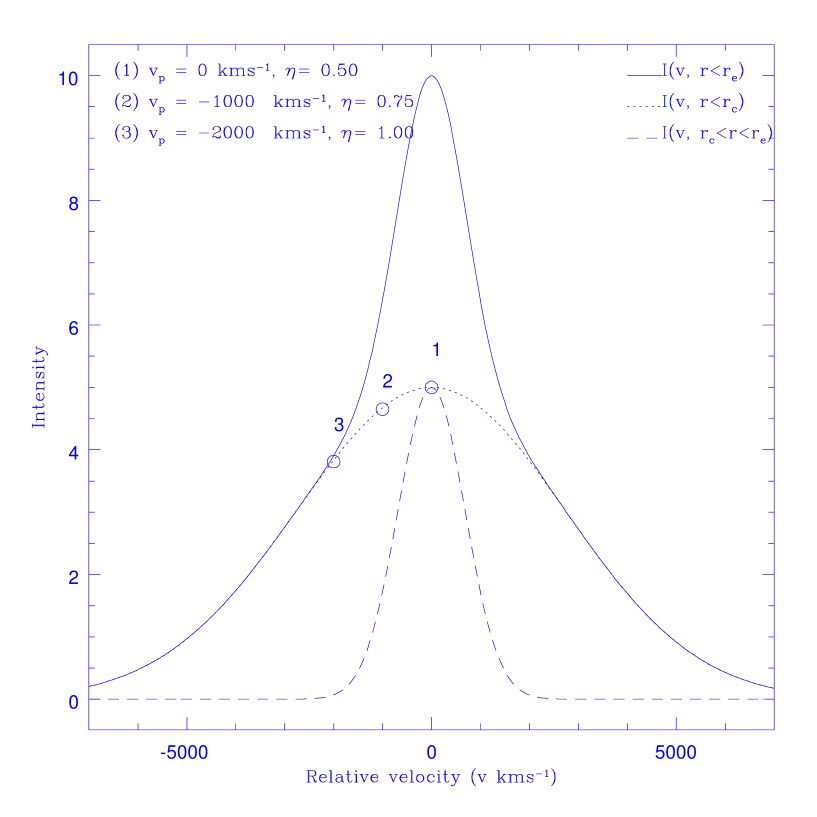
Figure 1: Simple illustration of the effect of peculiar velocity of the absorbing cloud, with respect to the AGN, on the observed covering factor.

The value of $\eta(v,r_{c})$ is going to depend on the radial dependent properties of the BLR such as (i) number of line emitting clouds per unit volume, (ii) ionization parameter (which is a dimensionless ratio of number of ionizing photons to the number of atoms), (iii) volume emissivity (iv) solid angle subtended by the emitting clouds on the central continuum source etc.. In the case of associated absorption lines the derived covering factor from the observations $\eta(v,r_{c})$ is going to be smaller than $f_{c}$ and the amount of departure for a given $r_{c}$ is decided by the peculiar velocity of the absorbing cloud with respect to the AGN. This effect can be understood using a simple illustration in Figure 1. The observed emission line (continuous curve) is decomposed into (a) emission produced within ’$r_{c}$’ and (b) emission from $r_{c}<r<r_{e}$ in the BLR (dashed line). For simplicity we assume the mean velocity of the second component is much less than the first component and both contribute equal amount to the observed intensity at $v=0$ $km~{}s^{-1}$ . If $z_{\rm abs}$= $z_{\rm em}$ (i.e $v_{p}=0$; marked as ’1’ in the figure) $\eta(0,r_{c})=0.50$. If the same cloud moves towards us with a velocity $v_{p}=1000$ $km~{}s^{-1}$  with respect to the background source (marked as ’2’ in the figure) then $\eta(-1000,r_{c})=0.75$. $\eta$ becomes 1 for any velocity greater than 2000 $km~{}s^{-1}$towards us.

Thus for a cloud covering the central region of the BLR the observed value of $\eta$ will be high if the absorption is present in the wings of the emission lines (with large peculiar velocity) compared to that if the absorption is present in the core of the emission lines (with small peculiar velocity). The case become interesting when we consider the doublets. For example C iv doublet has a velocity separation of $\sim$ 500 kms^-1. Thus $\eta$’s for both the lines are going to be different. Once again how different they can be is decided by the peculiar velocity of the cloud with respect to the AGN and the radial dependence of velocity distribution of the line emitting clouds in the BLR. The relationship between the residual intensities measured, in the case of the doublet, is

$$R_{2}~{}=~{}1~{}-~{}\eta_{2}~{}+~{}\eta_{2}\sqrt{{(R_{1}-1+\eta_{1})\over\eta_{1}}}$$ (8)

Thus the relationship between $R_{1}$ and $R_{2}$ are not unique and one can get different values of $R_{2}$ for a given value of $R_{1}$ by adjusting $\eta_{1}$ and $\eta_{2}$. Thus one needs three parameters to fit the doublets and an unique solution is not possible. The observed doublet ratio and its variations can either be a result of the difference in $\eta$’s for the doublet lines or a genuine column density effect. In the following subsections we discuss the implications of these two possibilities.

2.1 Variability in the column density

If the ionizing continuum varies with time scale, $t_{var}$, then the abundance of any ionization state, $i$, is given by the integrated creation rate of the stage, $i$, extended over a time, $t_{d}$, that is roughly the typical time scale for the destruction of an ion of state, $i$, either by recombination or ionization.

• 1. when $t_{d}<<t_{var}$: At any given time the ionization state is going to be in equilibrium with the ionizing radiation. Thus one can use simple photoionization model to predict the abundance of different ionization states as a function of continuum variability. In this case we will see a clear correlation or anti-correlation between the the continuum flux and the residual intensity (equivalent width) of the absorption line depending upon the ionization state under consideration.

  2. when $t_{d}\simeq t_{var}$: The ionic abundance follow a history that is smoothed and delayed version of the history of the ionizing flux. That is the residual intensity/equivalent width of the absorption line will follow the ionizing flux with a time delay. In this case the ionic abundances are neither in steady state nor in equilibrium.

  3. when $t_{d}>>t_{var}$: The ionic abundances reaches a steady state defined by the mean value of the ionization and recombination rates [over the time scale $\sim t_{d}$], but this steady state is almost never in equilibrium with the instantaneous value of the ionizing flux. In this case the equivalent width will remain constant and there will be no clear correlation (or anti-correlation) between the instantaneous value of the ionizing flux and the equivalent width. One can say there is no physical change in the absorber within the time scale $t_{var}$.

If the optical depth vary in response to the continuum variation over a time scale, $t_{var}^{1}$, then any variation in the continuum of similar magnitude over a time scale, $t_{var}>t_{var}^{1}$, should produce a similar variation in the column density. In the case of doublets if we assume the variation in the covering factor are negligible then,

$$\dot{R}_{1}~{}=~{}{2\eta_{1}\over\eta_{2}}~{}e^{-\tau_{1}/2}~{}\dot{R}_{2}.$$ (9)

As $\tau_{1}$ ($\sim 2\tau_{2}$) is inversely proportional to the ionization parameter,in the range of ionization parameter required for the intrinsic absorption systems, one would expect to see the residual intensity at any epoch anti-correlates with the continuum intensity and there should be a clear correlation between $\dot{R}_{1}$ and $\dot{R}_{2}$.

2.2 Variability in the covering factors

If we assume the absorbing cloud covers the central source emitting the continuum photons, then the line photon emitting clouds, within $r_{c}$, respond earlier to the variation in the continuum intensity compared to the clouds which are at a distance greater than $r_{c}$ from the center. If there is a momentary increase in the ionizing continuum emission, by $\delta(I_{o})$, that will produce a momentary increase in the $\eta(v,r_{c})$. Suppose the intensity of the ionizing radiation remains constant (at $I_{o}+\delta(I_{o})$) for the light travel time across the BLR the $\eta(v,r_{c})$, increases for a time equal to the light travel time over the distance $r_{c}$, then falls back to its original value. Here, we assume all the line emitting clouds are optically thick and emit isotropically in all direction. Since the light travel time across the BLR is 8 to12 days, any variation in the continuum intensity with a time scale less than this will produce variation in $\eta$ that will change the observed residual intensity in the bottom of the absorption line. Even if the optical depth, $\tau$, of the absorption line remains constant (or the variation in $\tau$ is very small) one would expect a variation in residual intensity due variation in $\eta$ and there will be a clear correlation between $\eta$ and residual intensity (and hence the equivalent width). Though the variations in the residual intensity are driven by the variations in the continuum luminosity there will be no correlation between the continuum luminosity and the measured residual intensity. Thus if we find the residual intensity change when the continuum vary over a time-scale, $t_{var}$ (which is less than the light travel time $t_{c}$ across $r_{c}$), then any variation in the continuum of similar magnitude over a time scale $t_{var}>t_{c}$ will not produce similar variation in the residual intensity.

In the case of doublets the variation in the residual intensities, $\dot{R}_{1}$ and $\dot{R}_{2}$, can be written in terms of variation in $\eta$’s ($\dot{\eta}_{1}$ and $\dot{\eta}_{2}$) as,

$$\dot{R_{1}}~{}=~{}\bigg{(}{{e^{-\tau_{1}}-1\over e^{-\tau_{2}}-1}}\bigg{)}~{}{\dot{\eta}_{1}\over\dot{\eta}_{2}}~{}\dot{R_{2}}$$ (10)

where $\tau_{1}~{}=~{}2\tau_{2}$. Here we have neglected the variation in the optical depth. The value of the ratio inside the bracket is positive and varies between 1 (when $\tau$ is very large) and 2 (when $\tau$ is very close to zero). Thus if the ratio of $\dot{R}_{1}$ to $\dot{R}_{2}$ is greater than 2 then we can conclude that $\dot{\eta}_{1}>\dot{\eta}_{2}$. Similarly if the ratio is less than 1 then we can say $\dot{\eta}_{1}<\dot{\eta}_{2}$. We do not expect to see any correlation between $\dot{R}_{1}$ and $\dot{R}_{2}$ in those cases were the variability is dominated by the change in $\eta$’s as the ratio of $\dot{\eta}_{1}$ by $\dot{\eta}_{2}$ need not be a constant. On time-scales much larger than the light travel time across the BLR the variability in the covering factor could be due to dynamical changes in the BLR or due to the motion of the absorbing cloud normal to the line of sight.

2.3 Probing the BLR using covering factor variability

If one finds a case in which the variability of the absorption line is dominated by the variability in covering factor then in principle using reverberation mapping techniques one can hope to infer,

• 1. whether the observed variability in the covering factor can naturally be produced by the light echo effects?

  2. the location of the absorbing clouds, and

  3. geometry and velocity structure of the BLR.

It is usually believed that the emission line photons are produced by the photoionization due to UV radiation from a central continuum source. It is a general procedure, in the ”reverberation mapping” studies, to express the observed line flux, $F_{l}(t)$, at any instant ${}^{\prime}t^{\prime}$ as a function of variation in the continuum flux ($F_{c}$) at earlier epochs ($t-\tau_{d}$), using the convolution equation given below.

$$F_{l}(t)=<F_{l}>+\int_{0}^{\tau(max)}d\tau~{}\psi(\tau_{d})[F_{c}(t-\tau_{d})-<F_{c}>]$$ (11)

Here, $<F_{l}>$, is the time averaged line flux and $<F_{c}>$ is the continuum mean (as defined by Krolik & Done, 1995) and is in general a function of the delay, $\tau_{d}$. $\psi$ is the response function (to be obtained by inverting the above integral equation), which describes the sensitivity of the line emissivity to continuum flux changes, integrated over the surface of constant delay.

The propagation of any change in the continuum through a spherical BLR is illustrated in Figure 2. The circles represent the constant delay surface with respect to the central source. The arrow gives the direction of the observer and the parabola are constant time delay surfaces (of time delay $\tau_{1}$, $\tau_{2}$ and $\tau_{3}$) as seen by an observer. Obtaining, $\psi(\tau_{d})$, using the emission line flux at any velocity interval, is nothing but integrating the sensitivity to the line emissivity of the clouds (having line of sight velocity in the range of our interest) present in a parabola of constant delay $\tau_{d}$ for a continuum variation that took place $\tau_{d}$ days before.

Let us suppose the vertical dashed line in Figure 2 represent the region covered by an absorbing cloud which is situated outside the BLR (as in the previous illustrations we assume the cloud covers the central continuum source and the central region of the BLR). In principle, by looking at the residual intensity in the bottom of the absorption lines, one can say whether the absorber is covering the continuum source or not. As can be seen from the figure, for small values of $\tau$, the response function obtained using the line emission, from the region covered by the absorbing cloud, will be similar to that obtained using the emission from the whole BLR. However at large delays, the value of $\psi$, obtained for the covered region will be much smaller. Thus $\tau(max)$ needed, to fit the variation in the line emission coming from the covered regions, will be smaller than the $\tau(max)$ needed for the total emission. How different they are will depend upon the distribution of line emitting clouds along our line of sight and their general radial distribution. $\tau(max)$ will provide an upper limit on the size of the absorbing region.

Since we know the emission line intensity in a velocity interval covered by the absorption line, from the fit to the emission line, we get the emission line intensity, at velocity ’$v$’, produced by the clouds in the BLR covered by the absorbing cloud using the calculated value of $\eta$ at that epoch. Thus one can get the transfer function for total emission from the BLR and the from the region covered by the absorption line. Careful analysis of these transfer functions will give more constraints on the BLR models than what one hope to infer from standard reverberation mapping studies.

3 Summary

In this work we describe a method of investigating the partial coverage of the background emitting region by an absorbing cloud, which will be very much for analysing the associated absorption seen in AGNs and QSOs. Using a simple minded example we illustrate how the complicated velocity structure in the BLR can alter covering factor of an absorption line. We also illustrate in general how lines of the doublets can have different covering factor as they cover different velocity range in a particular region of the BLR. We suggest how one can distinguish whether the variability seen in the absorption is due to variability in the optical depth or due to covering factor variability. We discuss how one can infer about the nature of the absorption system and the BLR using the standard reverbaration mapping technique and the observed variability in the covering factor.

Figure 2: Schematic diagram showing the iso-delay surfaces with respect to the central source (circles), and to an observer (parabola). The arrow shows the line of sight direction towards the observer and the region between the vertical dashed lines represent the region covered by an absorbing cloud towards the observer’s line of sight.

References

- (1) Barthel, P. D., et al. 1991, A&AS, 82, 339.
- (2) Bromage, G. E., et al. 1985, MNRAS, 215,1
- (3) Crenshaw, D. M. 1997, in ”Emission lines in Active galaxies: New methods and techniques”, eds. B. M. Peterson, F. Z. Cheng and A. S. Wilson (eds.), ASP conference Series, 113, 240.
- (4) Foltz, C. B.,Weymann, R.J., Peterson, B. M., Sun, L., Malkan, M. A., & Chaffee, Jr., F. H. 1986, ApJ, 307,504.
- (5) Kolman, M., et al. 1993, ApJ, 403, 592.
- (6) Koratkar, A., et a. 1996, ApJ, 470, 378.
- (7) Hamann, F. 1997, ApJS, 109, 279.
- (8) Hamann, F. et al., 1995, ApJ, 449, 603.
- (9) Hamann, F., Barlow, T. A., Junkkarinen, V., & Burbidge, E. M. 1997, ApJ, 478, 87.
- (10) Hamann, F., & Ferland, G. J. 1993, ApJ, 418,11.
- (11) Krolik, J., & Done, C. 1995, ApJ, 440, 166.
- (12) Maran, S.P., et al. 1996, ApJ, 465, 733.
- (13) Petitjean, P., Rauch, M., & Carswell, R. F. 1994, A&A, 291, 29.
- (14) Pogge, R. W., & Peterson, B. M. 1992, AJ, 103, 1084.
- (15) Sargent, W. L. W., Boksenberg, A., Steidel, C. C. 1988, ApJS, 68, 539.
- (16) Shull, J. M., & Sachs, E. R. 1993, ApJ, 416, 536.
- (17) Ulrich, M.H. 1988, MNRAS, 240, 833.
- (18) Walter, R. et al. 1990, A&A, 233,53.
- (19) weymann, R. J., Morris, S.L., Gray, M. E. & Hutchings, J. B. 1997, ApJ, 483, 717.
- (20) Weymann, R.J., Williams, R. E., Peterson, B. M., Turnshek, D. A. 1979, ApJ, 234, 33.