Solving the Flatness and Quasi-flatness Problems in Brans-Dicke Cosmologies with a Varying Light Speed

Abstract

We define the flatness and quasi-flatness problems in cosmological models. We seek solutions to both problems in homogeneous and isotropic Brans-Dicke cosmologies with varying speed of light. We formulate this theory and find perturbative, non-perturbative, and asymptotic solutions using both numerical and analytical methods. For a particular range of variations of the speed of light the flatness problem can be solved. Under other conditions there exists a late-time attractor with a constant value of $\Omega\$that is smaller than, but of order, unity. Thus these theories may solve the quasi-flatness problem, a considerably more challenging problem than the flatness problem. We also discuss the related $\Lambda$ and quasi-$\Lambda$ problem in these theories. We conclude with an appraisal of the difficulties these theories may face.

I The flatness and the quasi-flatness problems

The observable universe is close to a flat Friedmann model, the so-called Einstein-de Sitter universe, in which the energy density, $\rho,$ takes the critical value, $\rho_{c}$, and the homogeneous spatial surfaces are Euclidean. All astronomical evidence shows that we are quite close to this state of flatness, although a value of $\Omega_{0}$ in the vicinity of $0.2$ is preferred by several observations.

It is therefore disquieting to notice that the flat Friedmann model containing dust or blackbody radiation is unstable as time increases. Small deviations from the exact $\Omega=1$ model grow quickly in time, typically like $a^{2}$, where $a$ is the expansion factor of the universe. The observed $\Omega_{0}\approx 1$ state therefore requires extreme fine tuning of the cosmological initial conditions, assumed to be set at Planck epoch, because $a$ has increased by a factor of order $10^{32}$ from that epoch to the present. This is the flatness problem. If the universe is slightly open at Planck time, within a few Planck times it would become totally curvature dominated. If it is initially slightly closed, it would quickly collapse to Planck density again. Explaining its current state requires an extraordinarily close proximity to perfect flatness initially, or some sequence of events which can subsequently reverse expectations and render the flat solution asymptotically stable.

Particle physics theories naturally contain self-interacting scalar matter fields which violate the strong energy condition (so the density and pressure, $p$, obey $\rho+3p<0$). These can make the flat solution asymptotically stable with increasing time, allowing the asymptotic state to naturally be close to flatness. Cosmological histories in which a brief period of expansion is dominated by a matter field or other effective stress which violate the strong energy condition, and so exhibit gravitational repulsion, are called “inflationary”.

Solutions to the flatness problem have been proposed in the context of inflationary scenarios [1], pre-Big-Bang models [2], and varying speed of light cosmologies [3, 4, 5, 6]. In all of these theories, $\Omega=1$ becomes an asymptotically stable attractor for the expanding universe. The observed $\Omega_{0}\approx 1$ state results then from a temporary period of calculable physical processes, rather than from highly tuned initial conditions. In such scenarios the price to be paid is that $\Omega_{0}$ should be very close to unity, $\left|\Omega_{0}-1\right|$ $\leq 10^{-5}$, if one is not to invoke an unmotivated fine tuning of the initial conditions again.

If we take the trend of the observational data seriously, then explaining a current value of $\Omega_{0}$ of, say, $0.2-0.9$ is yet another challenge. We call it the quasi-flatness problem. Solutions to this problem have been proposed in the context of open inflationary models [14]. In these one has to come to grips with some degree of fine tuning. The Anthropic Principle [15] is usually invoked for this purpose [16] but considerable uncertainties exist in the range of predictions that emerge and there does not appear to be scope for a very precise prediction of $\Omega_{0}$ in, say, the range $0.2.$ Undoubtedly, it would be better if one could find mechanisms which would produce a definite $\Omega_{0}$ of order one, but different from 1, as an attractor. In a recent letter [8], we displayed one theory in which this possible. Here we present further solutions in support of such models. We explore analytical and numerical solutions to Brans-Dicke (BD) cosmologies with a varying speed of light (VSL). These generalise our earlier investigations of this theory [5, 6, 7]. We show that if the speed of light evolves as $c\propto a^{n}$ with $0<n<-1$ there is a late-time attractor at $\Omega=-n$. Hence, these cosmologies can solve the quasi-flatness problem. This work expands considerably the set of solutions presented in ref. [8].

We note that the existence of the dimensionless fine structure constants allows these varying-$c$ theories to be transformed, by a change of units, into theories with constant $c,$ but with a varying electron change, $e$, or dielectric ’constant’ of the vacuum. This process is described in detail in ref. [7] where a particular theory is derived from an action principle. A different varying-$e$ theory has been formulated by Bekenstein [11] but it is explicitly constructed to produce no changes in cosmological evolution. A study of this theory will be given elsewhere [12].

There also exist analogues of the flatness and quasi-flatness problems with regard to the cosmological constant. The lambda problem is to understand why the cosmological constant term, $\Lambda c^{2}$ in the Friedmann equation does not overwhelmingly dominate the density and curvature terms today (quantum gravity theories suggest that it ought to be about $10^{120}$ times bigger than observations permit [9, 15]). The quasi-lambda problem is to understand how it could be that this contribution to the Friedmann equation could be non-zero and of the same order as the density or curvature terms (as some recent supernovae observations suggest [10]).

In Section II we write down the evolution equations in these theories. The varying $G$ aspect of the theory will be accommodated in the standard way by means of a Brans-Dicke theory of gravitation. This theory is adapted in a well-defined way to incorporate varying $c.$ We write equations in both the Jordan and Einstein’s frames. In Section III we study solutions to the flatness problem in the perturbative regime ($\Omega\approx 1$), when both $c$ and $G$ may change. In Section IV we present non-perturbative solutions when $G$ is constant, and in Section V when $G$ is varying. In Section VI we derive simple conditions on any power-law variation of $c$ with scale factor if the flatness problem is to be solved. These conclusions are reinforced by some exact solutions in Section VII. In section VIII we show that the quasi-flatness problem can be naturally solved in a class of varying-$c$ cosmologies and then we discuss the solution of the quasi-lambda problem by such cosmologies in Section IX. We conclude with a summary of our results, highlighting the cases in which we can claim to have solved the quasi-flatness and quasi-lambda problems.

II Cosmological Field Equations

In BD varying speed of light (VSL) theories the Friedmann equations are [6]:

$$3{\frac{\ddot{a}}{a}} = -{\frac{8\pi}{(3+2\omega)\phi}}[(2+\omega)\rho+3(1+\omega)p/c^{2}]-\omega{\left(\frac{\dot{\phi}}{\phi}\right)}^{2}-{\frac{\ddot{\phi}}{\phi}}$$ (1)

$${\left(\frac{\dot{a}}{a}\right)}^{2} = {\frac{8\pi\rho}{3\phi}}-{\frac{Kc^{2}}{a^{2}}}-{\frac{\dot{\phi}a}{\phi a}}+{\frac{\omega}{6}}{\left(\frac{\dot{\phi}}{\phi}\right)}^{2}$$ (2)

where the speed of light, $c,$ is now an arbitrary function of time, $K$ is the curvature constant, and $\omega$ is the constant BD parameter. The wave equation for the BD scalar field $\phi=1/G$ is

$$\ddot{\phi}+3{\frac{\dot{a}}{a}}\dot{\phi}={\frac{8\pi}{3+2\omega}}(\rho-3p/c^{2})$$ (3)

From these three equations we can obtain the generalised conservation equation. Since after we impose the equation of state, the varying $c$ term only appears in eq. (2), the only new contribution to $2\dot{a}\ddot{a}$ is from the $-2Kc\dot{c}$ term. Hence, together, these imply the ’non-conservation’ equation:

$$\dot{\rho}+3{\frac{\dot{a}}{a}}(\rho+p/c^{2})={\frac{3Kc\dot{c}}{4\pi a^{2}}}\phi.$$ (4)

In the radiation-dominated epoch ($p=\rho c^{2}/3$) the general solution for $\phi$ is

$$\phi=\phi_{0}+\alpha{\int{\frac{dt}{a^{3}}}}$$ (5)

If the integration constant $\alpha=0$ the usual solutions for VSL in general relativity with varying $c$ follow illustrating the fact that for a radiation source any solution of general relativity is a particular solution of BD theory with constant $\phi$. In the next sections we explore the solutions to the flatness problem when $\dot{\phi}\neq 0$. We will also consider the radiation to matter transition in these theories.

Equations (1)-(5) apply in the so-called Jordan frame. It will be useful to introduce the Einstein frame, by means of the transformations,

$$d{\hat{t}} = {\sqrt{G\phi}}dt$$ (6)

$${\hat{a}} = {\sqrt{G\phi}}a$$ (7)

$$\sigma = {\left(\omega+3/2\right)}^{1/2}\ln({G\phi)}$$ (8)

$${\hat{\rho}} = (G\phi)^{-2}\rho$$ (9)

$${\hat{p}} = (G\phi)^{-2}p,$$ (10)

which are performed at constant $c$. These may be regarded as merely mathematical transformations of variables.

The Friedmann equations in the new frame are

$$3{\frac{{\hat{a}}^{\prime\prime}}{{\hat{a}}}} = {\frac{-4\pi G}{3}}[{\hat{\rho}}+3{\hat{p}}/c^{2}]-{\frac{\sigma^{\prime}{}^{2}}{3}}$$ (12)

$${\left(\frac{{\hat{a}}^{\prime}}{{\hat{a}}}\right)}^{2}+{\frac{Kc^{2}}{{\hat{a}}^{2}}} = {\frac{8\pi G{\hat{\rho}}}{3}}+{\frac{\sigma^{\prime}{}^{2}}{6}}$$ (13)

where ${}^{\prime}=d/d{\hat{t}}$. The transformed scalar field equation for $\sigma$ is

$$\sigma^{\prime\prime}+3{\frac{{\hat{a}}^{\prime}}{{\hat{a}}}}\sigma^{\prime}=-{\frac{8\pi G}{{\sqrt{6+4\omega}}}}({\hat{\rho}}-3{\hat{p}}/c^{2})$$ (14)

These are just the standard Friedmann equations with constant $G$ and a scalar field added to the normal matter. The scalar field behaves like a ’stiff’ perfect fluid with equation of state

$${\hat{p}}_{\sigma}={\hat{\rho}}_{\sigma}={\frac{\sigma^{\prime}{}^{2}}{16\pi G}.}$$ (15)

In the Einstein frame, if $\dot{c}=0$, the total stress-energy tensor is conserved, but the scalar field and normal matter exchange energy according to:

$${\hat{\rho}}^{\prime}+3{\frac{{\hat{a}}^{\prime}}{{\hat{a}}}}({\hat{\rho}}+{\hat{p}}/c^{2})=-({\hat{\rho}}_{\sigma}^{\prime}+3{\frac{{\hat{a}}^{\prime}}{{\hat{a}}}}({\hat{\rho}}_{\sigma}+{\hat{p}}_{\sigma}/c^{2}))={\frac{\sigma^{\prime}({\hat{\rho}}-3{\hat{p}}/c^{2})}{{\sqrt{6+4\omega}}}.}$$ (16)

If $\dot{c}\neq 0,$ one has instead

$${\hat{\rho}}^{\prime}+3{\frac{{\hat{a}}^{\prime}}{{\hat{a}}}}({\hat{\rho}}+{\hat{p}}/c^{2}) = {\frac{\sigma^{\prime}({\hat{\rho}}-3{\hat{p}}/c^{2})}{{\sqrt{6+4\omega}}}}+{\frac{3Kc^{2}}{4\pi G{\hat{a}}^{2}}}{\frac{c^{\prime}}{c}}$$ (17)

$${\hat{\rho}}_{\sigma}^{\prime}+3{\frac{{\hat{a}}^{\prime}}{{\hat{a}}}}({\hat{\rho}}_{\sigma}+{\hat{p}}_{\sigma}/c^{2}) = -{\frac{\sigma^{\prime}({\hat{\rho}}-3{\hat{p}}/c^{2})}{{\sqrt{6+4\omega}}}}$$ (18)

All equations derived for standard VSL theory, with constant $G$, are valid in the Einstein frame. However, one should always remember to add to normal matter the scalar field energy and pressure (so the total density and pressure are given by ${\hat{\rho}}_{t}={\hat{\rho}}+\rho_{\sigma}$ and ${\hat{p}}_{t}={\hat{p}}+{\hat{p}}_{\sigma},$ respectively).

III Perturbative solutions to the flatness problem

We first study solutions to the flatness problem when there are small deviations from flatness. Let us define the critical density, $\rho_{c}$ , in a B-D universe by means of the equation:

$${\left(\frac{\dot{a}}{a}\right)}^{2}={\frac{8\pi\rho_{c}}{3\phi}}-{\frac{\dot{\phi}a}{\phi a}}+{\frac{\omega}{6}}{\left(\frac{\dot{\phi}}{\phi}\right)}^{2},$$ (19)

that is, Eqn. 2 with $K=0$. In the Einstein frame the critical density in normal matter is

$${\hat{\rho}}_{c}={\frac{3}{8\pi G}}{\left({\left(\frac{{\hat{a}}^{\prime}}{{\hat{a}}}\right)}^{2}-{\frac{{\sigma^{{}^{\prime}2}}}{6}}\right)}={\frac{\rho_{c}}{G^{2}\phi^{2}}}$$ (20)

In terms of total energy density ${\hat{\rho}}_{t}={\hat{\rho}}+\rho_{\sigma}$ , the critical energy density in the Einstein frame is:

$${\hat{\rho}}_{ct}={\frac{3}{8\pi G}}{\left(\frac{{\hat{a}}^{\prime}}{{\hat{a}}}\right)}^{2}.$$ (21)

Accordingly, we may define a relative flatness parameter:

$${\hat{\epsilon}}_{t}={\frac{{\hat{\rho}}_{t}-{\hat{\rho}}_{ct}}{{\hat{\rho}}_{ct}}}$$ (22)

As shown in the previous section, the usual equations for VSL theory should apply to this quantity. Therefore, one has

$${\hat{\epsilon}_{t}}^{\prime}=(1+{\hat{\epsilon}}_{t}){\hat{\epsilon}}_{t}(3\gamma-2){\frac{{\hat{a}}^{\prime}}{{\hat{a}}}}+2{\frac{c^{\prime}}{c}}{\hat{\epsilon}}_{t}$$ (23)

with the equation of state given by

$$\gamma-1\equiv p/\rho c^{2}={\hat{p}}/{\hat{\rho}}c^{2}$$ (24)

with $\gamma$ constant.

But, since

$${\hat{\epsilon}}_{t}={\frac{\epsilon}{1+(2\omega+3){\frac{{\dot{\phi}}^{2}}{8\pi\phi\rho_{c}}}},}$$ (25)

we see that the natural quantity to quantify deviations from flatness in the Jordan frame is not

$$\epsilon={\frac{{\rho}-{\rho}_{c}}{{\rho}_{c}}}$$ (26)

but an adaptation of it,

$$\delta={\frac{\rho-\rho_{c}}{\rho_{c}+{\frac{(2\omega+3){\dot{\phi}}^{2}}{8\pi\phi}}}}<\epsilon,$$ (27)

which satisfies the equation

$$\dot{\delta}=(1+\delta)\delta(3\gamma-2){\left({\frac{\dot{a}}{a}}+{\frac{1}{2}}{\frac{\dot{\phi}}{\phi}}\right)}+2{\frac{\dot{c}}{c}}\delta.$$ (28)

If $\delta\ll 1$ this can be integrated to give

$$\delta\propto a^{3\gamma-2}c^{2}\phi^{\frac{\ 3\gamma-2}{2}}$$ (29)

Hence, we have the solution

$${\frac{1}{\epsilon}}={\frac{C}{a^{3\gamma-2}c^{2}\phi^{\frac{3\gamma-2}{2}}}}-{\frac{(2\omega+3){\dot{\phi}}^{2}}{8\pi\phi\rho_{c}}.}$$ (30)

If $G\propto\phi^{-1}$ varies then the second term on the right always works against solving the flatness problem. Hence solving the flatness problem in BD requires that $\phi$ decreases in the early universe and that the first term on the right of eq. (30) dominates the second.

In a radiation-dominated universe ($\gamma=4/3$):

$${\frac{1}{\epsilon}}={\frac{C}{a^{2}c^{2}\phi^{2}}}-{\frac{(2\omega+3){\alpha}^{2}}{8\pi\phi a^{6}\rho_{c}},}$$ (31)

where $\alpha$ was defined by eqn.(5). If $\alpha$ is small and $c=c_{0}a^{n}$ one still solves the flatness problem when $n<-1$. Notice that since $\rho_{c}\propto 1/a^{4}$ at late times, the second term always eventually becomes negligible.

IV Non-perturbative solutions with $\phi=const$

A Matter and radiation-dominated cases

In order to explore non-perturbative solutions to the flatness problem we solved Eqns. (1)-(5) numerically. First we consider the case where $\phi=\phi_{0}$. Exact solutions exist in this case for matter and radiation-dominated universes. Setting $\phi=1/G$ in Eqn. (28) leads to

$${\dot{\epsilon}}=(1+\epsilon)\epsilon(3\gamma-2){\frac{{\dot{a}}}{{a}}}+2{\frac{{\dot{c}}}{c}}\epsilon$$ (32)

which, assuming ${\dot{c}}/c=n{\dot{a}}/a,$ becomes

$${\dot{\epsilon}}=\epsilon{\left((1+\epsilon)(3\gamma-2)+2n\right)}{\frac{{\dot{a}}}{{a}}.}$$ (33)

The general structure of the attractors can be inferred from this equation. However, it can also be integrated to give

$$\epsilon=-{\frac{1+{\frac{2n}{3\gamma-2}}}{1-Ca^{-(2n+3\gamma-2)}},}$$ (34)

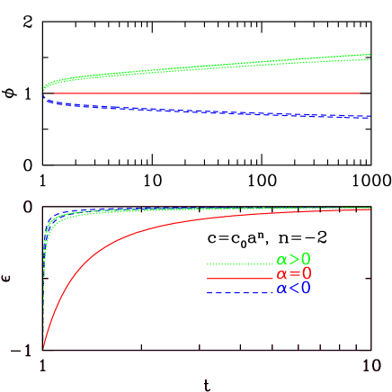
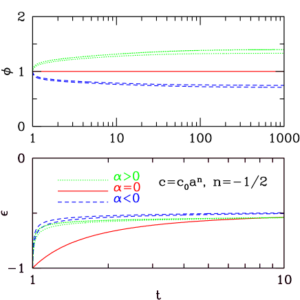
with $n<0$, and where the integration constant $C$ is chosen so as to enforce the specified initial conditions. Our numerical code matched this analytical result to very high accuracy. In Fig. 1 we plot numerical results for a radiation-dominated universe. We comment on four possible situations, illustrated in Figs. 1-4.

FIG. 1.: The evolution of $\epsilon$ from various initial values for cosmologies with $\phi=const$ and $c=c_{0}$. We see that the flat universe is unstable.

FIG. 2.: The VSL solution to the flatness problem. We have assumed a radiation-dominated universe, and considered a situation with $n<-(3\gamma-2)/2$. We see that although the flat universe is now an attractor, if the universe is ever too closed it will end in a Big Crunch, rather than approach the flat attractor.

FIG. 3.: The VSL solution to the quasi-flatness problem. We have assumed a radiation-dominated universe, and considered a situation with $-(3\gamma-2)/2<n<0$. The attractor is now at a value of $\Omega$ of order 1, but not necessarily 1. Closed universes end up in a Big Crunch, but any open universes are pushed towards $\Omega=-2n/(3\gamma-2)$.

 

FIG. 4.: The transition case $n=-(3\gamma-2)/2$ illustrated for a radiation dominated Universe.

If $c$ is a constant ($n=0$) then the flat universe ($\epsilon=0$) is unstable (Fig. 1). There are two attractors at $\epsilon=-1$ and $\epsilon=\infty$, showing that the universe tends to become curvature dominated. For slightly closed universes this means evolution towards a Big Crunch singularity. For slightly open universes it means evolution towards a Milne universe ($\epsilon=-1$) which in the case of constant $G$ is simply an expanding empty spacetime with $a\propto t$. If the speed of light were to increase with $a$ ($c\propto a^{n}$ with $n>0$) the situation is the same, but with a stronger repulsion from $\epsilon=0$.

If $c\propto a^{n}$ with $n<-(3\gamma-2)/2$, then, as pointed out in [6], the flatness problem is solved if $\epsilon$ is not too far from zero initially. In fact, $\epsilon=0$ is now an attractor (see Fig. 2). The non-perturbative analysis reveals two novelties: there is an unstable node at $\epsilon=-1-2n/(3\gamma-2)$ and $\epsilon=\infty$ is an attractor. This means that if the universe at any given initial time satisfies $\epsilon>-1-2n/(3\gamma-2)$ it will not evolve towards the flat attractor. Instead, it will evolve towards a big crunch with $\epsilon=\infty$. Therefore, for closed universes, the flatness problem is solved only if they are not too positively curved.

It is curious to note that the situation is different for open universes. No matter how far they are from flatness they will always evolve towards the Einstein-de Sitter model at late times. This was first pointed out in [5], where it was noted that in VSL theories the Einstein-de Sitter universe is an attractor even if the universe is initially Minkowski (empty) or de Sitter (dominated by a cosmological constant).

The greatest novelty, however, appears for the case in which $-(3\gamma-2)/2<n<0$. Although $\epsilon=0$ is now unstable, there is a stable attractor at $\epsilon=-1-2n/(3\gamma-2)$ (see Fig. 3). The system is now repelled from $\epsilon=-1$ but is attracted to $\epsilon=\infty$.

Hence we have the following scenario: all closed universes evolve towards a big crunch, no matter how close to flatness they are initially. Thus a selection process excludes even slightly closed universes.  In contrast, flat and all open models (no matter how low their density) evolve towards an open model with $\Omega=-2n/(3\gamma-2)$, a value that lies between $0$ and $1$, and is typically of order unity. We therefore have a solution to the quasi-flatness problem, for open, but not for closed universes.

The $n=-(3\gamma-2)/2$ case is a transition case in between the last two situations just described (Fig. 4). In this case $\epsilon=0$ is a saddle: stable if approached from below but unstable from above.

B The radiation-to-matter transition

In quasi-flat scenarios the major contribution to the matter density of the universe is the term resulting from violations of energy conservation. This can be seen from

$$\rho=\frac{B}{a^{3\gamma}}+\frac{3Kc_{0}^{2}\phi n}{4\pi(3\gamma+2n-2)}a^{2n-2}$$ (35)

derived above. Taking radiation as an example ($\gamma=4/3$), if $n<-1$ we are pushed towards the attractor $\Omega=1$ and the energy-violation term (second term) becomes negligible. In scenarios in which the quasi-flatness problem is solved the converse happens: the second term dominates. Matter is continuously being created and this provides the dominant contribution to cosmic matter at any given time. Matter which was created in the past gets diluted away by expansion very quickly. In effect, we have a state of permanent “reheating”. This scenario has a passing resemblance with the steady state universe, in which the so called $C$ field continuously creates more and more matter.

If we couple a changing $c$ say to the Lagrangian of the standard particle physics model then all particles are produced, and whether they behave like matter or radiation depends on whether $T\ll m$ or $T\gg m$. If $n<0$ the energy density in created matter decreases, and the universe cools down as it expands. Hence there will necessarily be a radiation to matter transition in these scenarios, just like in the standard Big Bang theory with constant $G$ and $c$.

A complication arises when we attempt to model the evolution through this transition because the structure of the attractors changes. For a radiation-dominated universe one requires $-1<n<0$ for the open attractor $\Omega=-n$ to be achieved. For a matter-dominated universe the attractors for open universes are given by $\Omega=-2n$ and are achieved when $-1/2<n<0$. Hence, if $-1<n<-1/2$ we have attraction towards a (quasi-flat) open universe during the radiation-dominated epoch which is then driven towards flatness in the subsequent matter-dominated epoch. If $-1/2<n<0$ we have attraction to a (quasi-flat) open model in both epochs but the universe will evolve from a trajectory asymptoting to $\Omega=-n$ toward one asymptoting to $\Omega=-2n$ after the matter-radiation equality time. The solution (34) is then no longer valid because $\gamma$ is time dependent.

V Solutions with variable $\phi$

A Exact Radiation solutions

For radiation, $\gamma=4/3$, we can solve the field equations by generalising the method introduced for scalar-tensor theories introduced in ref. [13]. Define the conformal time

$$ad\tau=dt$$ (36)

so ${}^{\prime}=d/d\tau.$ Eq. (3) integrates to give

$$\phi^{\prime}=\frac{A}{a^{2}}$$ (37)

with $A$ constant .

Now change the variables of eq.(2) by introducing

$\displaystyle y=\phi a^{2}$

and $d/d\tau.$ It reduces to

$$y^{\prime 2}=A^{2}(1+\frac{2\omega}{3})+\frac{32\pi y\rho a^{4}}{3}-4Kc^{2}y^{2}$$ (38)

For radiation, eq. (59) gives

$$\rho a^{4}=B+\frac{3Kc_{0}^{2}my^{2m+1}}{4\pi(2m+1)}$$ (39)

If we substitute (39) in (38) then we have

$$y^{\prime 2}=A^{2}(1+\frac{2\omega}{3})+\frac{32\pi B\ }{3}y+4Kc_{0}^{2}[\frac{2m}{\ (2m+1)}-1]\ y^{2(m+1)}$$ (40)

This can be integrated exactly for appropriate choices of $m$ and its qualitative behaviour is easy to understand. Note that if we can solve (40) for $y(\tau)$ $=\phi a^{2}$, then we know $\phi(\tau,a)$ and can solve (37) to get $\phi(\tau)$ hence $a(\tau),$ and finally $a(t)$ from (36) since

$$\frac{\phi^{\prime}}{\phi}=\frac{A}{y}$$ (41)

We note that the curvature term in (40) changes sign for a special value of $m,$

$\displaystyle m=m_{*}=-\frac{1}{2}$

Examining (40) we see that the $K=0$ solution appears to be approached if $2(m+1)<1$, ie $m<-1/2.$

When $m=-1$ there is a simple special case which allows an exact solution. Eq. (40) is now

$$y^{\prime 2}=\alpha+\beta y+\Gamma$$ (42)

where $\alpha,\beta>0,\Gamma=+4Kc_{o}^{2}.$ We integrate (41) to get

$$y=\frac{\beta}{4}(\tau+\tau_{0})^{2}-\frac{\alpha+\Gamma}{\beta}=\phi a^{2}$$ (43)

Hence,

$\displaystyle\phi=\phi_{0}\left[\frac{\beta(\tau+\tau_{0})-2\sqrt{\alpha+\Gamma}}{\beta(\tau+\tau_{0})+2\sqrt{\alpha+\Gamma}}\right]^{A/\sqrt{\alpha+\Gamma}}$

and

$\displaystyle a^{2}=\frac{y}{\phi}=\frac{\beta^{2}(\tau+\tau_{0})^{2}}{4\beta\phi_{0}}\left[\frac{\beta(\tau+\tau_{0})+2\sqrt{\alpha+\Gamma}}{\beta(\tau+\tau_{0})-2\sqrt{\alpha+\Gamma}}\right]^{A/\sqrt{\alpha+\Gamma}}$

We see that if $\alpha+\Gamma>0$ then, as $\tau\rightarrow\infty,$ we have $a\rightarrow\tau\rightarrow t^{1/2}$ unless the denominator blows up.

If $\alpha+\Gamma<0$ then we get

$\displaystyle\ln(\phi/\phi_{0})=\frac{2A}{\sqrt{-(\alpha+\Gamma)}}\tan^{-1}\left(\frac{\beta(\tau+\tau_{0})}{\sqrt{-(\alpha+\Gamma)}}\right)$

and

$\displaystyle a^{2}=\frac{1}{4\phi_{0}\beta}\left[\beta^{2}(\tau+\tau_{0})+\lambda^{2}\right]\exp\{-\frac{4A}{\lambda}\tan^{-1}\left(\frac{\beta(\tau+\tau_{0})}{\lambda}\right)\}$

where

$\displaystyle\lambda^{2}\equiv-4(\alpha+\Gamma)$

Looking back at the defining equation (40), we see that for this $m=-1$ case, $\Gamma=4Kc_{0}^{2}$ and so

$\displaystyle\alpha+\Gamma=A^{2}(1+\frac{2\omega}{3})+4Kc_{0}^{2}\$

and for large $A$ we have $\alpha+\Gamma>0$ when $K>0$.

B Numerical solutions

A numerical evolution of the equations with a varying $\phi$ reveals that for reasonable initial values of $\phi$ the structure of attractors is not affected. However, the speed at which attractors are reached may be increased if $\phi$ is allowed to change. As an example we shall consider the case in which one starts from a Milne universe ($\epsilon=-1$). In [5] it was argued that this is the natural initial condition to consider in the context of VSL cosmologies.

Let us then consider the case $\gamma=4/3$, and integrate Eqns. (1 ), (2), and (3). We consider solutions of the form (5) with various integration constants $\alpha$. In Figures 5 and 6 we show the evolution of $\epsilon=\Omega-1$ and $\phi$ from such a state, with $c=c_{0}a^{n}$ and $n=-2,-1/2$. In the first case we see that we still have a flat attractor, which is reached much more rapidly if $\phi$ is increasing or decreasing. In the latter case we have a quasi-flat attractor, with $\epsilon=-1/2$, whether or not $\phi$ is allowed to change. The attractor is achieved faster with a changing $\phi$, especially a decreasing one.

FIG. 5.: The evolution of $\epsilon=\Omega-1$ and of $\phi=1/G$ from a Milne starting point, with $\gamma=4/3$, $c=c_{0}/a^{2}$, and different values of the integration constant $\alpha,$ of eq. (5). We see that flatness is achieved faster with a changing $G$ (increasing or decreasing).

FIG. 6.: The quasi-flat scenario with VSL and a changing $G$. We consider a Milne starting point, with $\gamma=4/3$, $c=c_{0}/a^{1/2}$, and different integration constants $\alpha$. The quasi-flat attractor is still the same as in the constant $\phi$ case, but it is achieved faster with a changing $\phi$ (especially a decreasing one).

VI Asymptotic Solutions to the Flatness Problem

Exact solutions are only possible for particular equations of state and $c$-variation laws but it is possible to understand the asymptotic behaviour in general. The VSL theory Brans-Dicke solutions are given for eqns. (1)-(3) together with (4). We assume a perfect-fluid equation of state given by (24). In the flat case ($K=0$) the equations reduce to those of standard BD flat universes with constant $c$. At late times, when $K=0$, the general BD solutions for all $\gamma$ approach the particular (’matter-dominated’ or ’Machian’) power-law solutions [17]

$$G \propto \phi^{-1}\propto t^{-D}$$ (44)

$$a(t) \propto t^{A}$$ (45)

where

$$A=\frac{2+2\omega(2-\gamma)}{\begin{array}[]{c}4+3\omega\gamma(2-\gamma)\\ \end{array}}$$ (46)

$$D=\frac{2(4-3\gamma)}{\begin{array}[]{c}4+3\omega\gamma(2-\gamma)\\ \end{array}}$$ (47)

Hence, we see that $D+3\gamma A=2;$ note that $D=0$ for radiation;.These exact power-law solutions reduce the special $\phi=const,a\propto t^{1/2}$ general relativity solution in the radiation case. We shall therefore look at the stability of these $K=0$ asymptotes when we turn on the $K\neq 0$ terms in eqns. (1)-(3) and (4) with $c(t)$ included. If we substitute (46) and (47) in (4) with $c=c_{0}a^{n}$ then we have

$$(\rho t^{3\gamma A})^{\cdot} \simeq \frac{3Kc_{0}^{2}An\phi_{0}}{4\pi}t^{A(3\gamma+2n-3)+A-1+D}\simeq\frac{3Kc_{0}^{2}An\phi_{0}}{4\pi}t^{1+2A(n-1)}$$

Integrating, we get

$$\rho t^{3\gamma A}\simeq B+\frac{3Kc_{0}^{2}An\phi_{0}}{8\pi(1+An-A)}t^{2(1+An-A)}$$ (48)

if $A(n-1)\neq-1$. Thus, to solve the flatness problem we will need the $B$ term to dominate the $K$ term on the right-hand side of eq. (48) at large $t;$ that is, since $A>0$ for expanding universes, asymptotic approach to flatness requires

$\displaystyle n<1-\frac{1}{A}.$

Using (46), this gives the condition

$\displaystyle n<\frac{(2-\gamma)(2-3\gamma)\omega-2}{2[1+\omega(2-\gamma)]}.$

For radiation and dust universes this condition for solving the flatness problem reduces to:

$$rad : n<-1$$ (49)

$$dust : n<\frac{-(\omega+2)}{2(\omega+1)}\rightarrow-\frac{1}{2}\ as{\rm{\ }\omega\rightarrow\infty}$$ (50)

where (50) approaches the general relativity value for $\omega\rightarrow\infty,$ as expected and (49) agrees with the radiation case studied above.

VII Exact solutions to the flatness problem

A Radiation-dominated case

The exact solutions found for the VSL theory with $c=c_{0}a^{n}$ in [6] can be generalized to the BD case if one assumes that the variation of the speed of light is governed by a relation of the form

$$c=c_{0}(a\sqrt{G\phi})^{n}$$ (51)

This reduces to the previously studied (non-BD) case when $\phi$ is constant. In the Einstein frame one then has $c=c_{0}{\hat{a}}^{n}$ and in the radiation-dominated epoch the first of equations (17) becomes

$${\hat{\rho}}^{\prime}+3{\frac{{\hat{a}}^{\prime}}{{\hat{a}}}}({\hat{\rho}}+{\hat{p}}/c^{2})={\frac{3Kc^{2}}{4\pi G{\hat{a}}^{2}}}{\frac{c^{\prime}}{c}}$$ (52)

Hence, for radiation, one has the integral

$${\hat{\rho}}{\hat{a}}^{4}=B+{\frac{3Kc_{0}^{2}n{\hat{a}}^{2n+2}}{4\pi G(2n+2)}}$$ (53)

with $B$ constant. Since ${\hat{\rho}}{\hat{a}}^{4}=\rho a^{4},$ in the Jordan frame, one has

$$\rho a^{4}=B+{\frac{3Kc_{0}^{2}na^{2n+2}(G\phi)^{n+1}}{4\pi G(2n+2)}}$$ (54)

This solution can be verified directly from eq. (4), although it would have been difficult to guess it without a foray into the Einstein frame.

Conditions for solving the flatness problem can now be derived by inspection of the Friedmann-like equation:

$${\left(\frac{\dot{a}}{a}\right)}^{2}={\frac{C_{1}}{\phi a^{4}}}+{C_{2}Ka^{2n-2}\phi^{n}}-{KC_{3}a^{2n-2}\phi^{n}}-{\frac{\dot{\phi}a}{\phi a}}+{\frac{\omega}{6}}{\left(\frac{\dot{\phi}}{\phi}\right)}^{2}$$ (55)

Since $\phi$ approaches an asymptotic value we still require that $n<-1$ for the term in $C_{1}$ to dominate the curvature ($K$) term at late times.

If $\phi$ is decreasing we do not need the speed of light to decrease in time so fast in order to solve the flatness problem. Since

$${\frac{\dot{c}}{c}}=n{{\frac{\dot{a}}{a}}+{\frac{1}{2}}{\frac{\dot{\phi}}{\phi}}}$$ (56)

we see that while ${\dot{\phi}/\phi}$ is non-negligible we have $|\dot{c}/c|<|n|\dot{a}/a$. Weaker gravity in the early universe therefore assists a varying speed of light in solving the flatness problem

B Other equations of state

Introduce the variable

$$x=\phi a^{3\gamma-2\ }$$ (57)

and assume that $c$ varies as

$$c=c_{0}x^{n/2}$$ (58)

Hence, (69) becomes

$\displaystyle(\rho a^{3\gamma})^{\cdot}=\frac{3Kc_{0}^{2}n}{8\pi}x^{n}\dot{x}$

Integrating, we have

$$\rho a^{3\gamma}=B+\frac{3Kc_{0}^{2}n\phi^{n+1}a^{(3\gamma-2)(n+1)}}{8\pi(n+1)}$$ (59)

if $n\neq-1$. This solution can be used to study the evolution for general $\gamma.$

VIII Solutions to the Quasi-flatness Problem

A The constant $\phi$ case

We want to discover if it is ever natural to have evolution which asymptotes to a state of expansion with a non-critical density (for example, say, $\Omega_{0}\simeq 0.2,$ as some observations have implied). For simplicity we consider first the solutions with constant $\phi.$ The conservation equation (4) with constant $\phi$ reduces to

$$\frac{(\rho a^{3\gamma})^{\cdot}}{a^{3\gamma}} = \frac{3Kc_{0}^{2}n}{4\pi}a^{2n-3}\dot{a}\phi$$

which integrates to give

$$\rho=\frac{B}{a^{3\gamma}}+\frac{3Kc_{0}^{2}\phi n}{4\pi(3\gamma+2n-2)}a^{2n-2}$$ (60)

with $B$ constant, so substituting in (2) we have

$\displaystyle\frac{\dot{a}^{2}}{a^{2}}=\frac{8\pi B}{3\phi a^{3\gamma}}-\frac{K(3\gamma-2)c_{0}^{2}\ }{a^{2(1-n)}(3\gamma+2n-2)}.$

¿From this we can easily determine the attractors at large $a$. Specialising to the radiation case, we have

$\displaystyle\frac{\dot{a}^{2}}{a^{2}}=\frac{8\pi B}{3\phi a^{4}}-\frac{K\ c_{0}^{2}\ }{a^{2(1-n)}(1+n)}.$

Now, the density parameter $\Omega$ is defined by:

$${\frac{\Omega}{\Omega-1}}={\frac{\frac{8\pi G\rho}{3}}{\frac{Kc^{2}(t)\ }{a^{2}}}}$$ (61)

For a quasi-flat open universe the ratio between the two terms on the right-hand side is approximately constant. From the solution (60) with $\gamma=4/3$ we have

$${\frac{\Omega}{\Omega-1}}={\frac{\frac{8\pi G}{3}{\left({\frac{B}{a^{4}}}+{\frac{3Kc_{0}^{2}n}{8\pi G(n+1)a^{2(1-n)}}}\right)}}{\frac{Kc_{0}^{2}}{a^{2(1-n)}}}}$$ (62)

If $n<-1$ the energy production term (second term on the right-hand side of ( 60)) is subdominant at late times, and so this ratio goes to infinite, meaning $\Omega=1$. If $0<n<-1$ then the second term in (60 ) dominates at late times and therefore the expansion asymptotes to one displaying

$${\frac{\Omega}{\Omega-1}}={\frac{n}{n+1}}$$ (63)

that is $\Omega=-n$. So the key feature is that in these scenarios the curvature terms associated with violations of energy conservation dump energy into the universe at the same rate as the curvature term in Friedmann equation. Therefore the ratio of the two terms in the Friedmann equation stays constant, leading to an open universe with finite $\Omega$ value today.

B The varying $\phi$ case

The formulation of the radiation case in terms of the variable $y(\tau)=\phi a^{2}$ allows us to extend the analysis to the varying-$\phi$ case. Taking

$$c=c_{0}y^{m}$$ (64)

we have

$$y^{\prime 2}=A^{2}(1+\frac{2\omega}{3})+\frac{32\pi y\rho a^{4}}{3}-4Kc^{2}y^{2}$$ (65)

and

$$\rho a^{4}=B+\frac{3Kc_{0}^{2}my^{2m+1}}{4\pi(2m+1)}.$$ (66)

We introduce the density parameter

$\displaystyle\Omega=\frac{\rho}{\rho_{c}}=\frac{y^{\prime 2}-A^{2}(1+\frac{2\omega}{3})+4Kc^{2}y^{2}}{y^{\prime 2}-A^{2}(1+\frac{2\omega}{3})\ },$

so that

$\displaystyle\frac{\Omega}{\Omega-1}=\frac{8\pi}{3Kc_{0}^{2}y^{2m+1}}\left[B+\frac{3Kmc_{0}^{2}y^{2m+1}}{4\pi(2m+1)}\right].$

As $t\rightarrow\infty,\tau\rightarrow\infty,y\rightarrow\infty$ we see that $\Omega\rightarrow 1$ if $2m+1<0$ (in Section V we give a full exact solution for the case $m=-1$ which falls into this class), but if $2m+1>0$ we have approach to a quasi-flat open universe with

$\displaystyle\Omega\rightarrow-2m$

Again, we can have a natural quasi-flat asymptote with $0<\Omega<1.$

C General asymptotic behaviour

Consider the behaviour of eq. (40) at large $\tau$ and $y$ in the case where $2m+1>0;$ that is, where we have the quasi-flat attractor $\Omega\rightarrow\Omega_{\infty}=-2m$ as $\tau\rightarrow\infty.$ This assumes the constants in the Friedmann equation allow sufficient expansion to occur (so there is no collapse at a finite early time). Since

$\displaystyle y^{\prime}\simeq\Gamma y^{m+1}$

we have

$\displaystyle y\simeq\left[\frac{\Gamma\Omega_{\infty}}{2}(\tau+\tau_{0})\right]^{\frac{2}{\Omega_{\infty}}}\sim\tau^{\frac{2}{\Omega_{\infty}}}$

as $\tau\rightarrow\infty.$ Using (41) we get

$\displaystyle\phi=\phi_{0}\exp\left[\frac{\tau^{1-\frac{2}{\Omega_{\infty}}}}{1-\frac{2}{\Omega_{\infty}}}\right]$

so, since $\Omega_{\infty}<1$, we have $\phi\rightarrow\phi_{0}$ as $\tau\rightarrow\infty.$ So, we have

$\displaystyle a(\tau)\sim\tau^{\frac{1}{\Omega_{\infty}}}\exp\left[\frac{\tau^{1-\frac{2}{\Omega_{\infty}}}}{2(1-\frac{2}{\Omega_{\infty}})}\right]\sim\tau^{\frac{1}{\Omega_{\infty}}}$

Thus $t\sim\tau^{(\Omega_{\infty}+1)/\Omega_{\infty}}$ and

$\displaystyle a\sim t^{\frac{1}{(1+\Omega_{\infty})}}$

as $t\rightarrow\infty.$ When $\Omega_{\infty}=1$ we have the expected $a\sim t^{\frac{1}{2}}$ flat radiation asymptote.

IX The Lambda and the Quasi-lambda Problems

A The General Relativity Case

Let us consider the impact of a varying speed of light on the general relativity case. Similar results will occur in the BD case (to which it reduces exactly in the case of radiation with constant $\phi$). If we wish to incorporate a cosmological constant term, $\Lambda$, (which we shall assume to be constant) then we can define a vacuum stress obeying an equation of state

$$p_{\Lambda}=-\rho_{\Lambda}c^{2},$$ (67)

where

$$\rho_{\Lambda}=\frac{\Lambda c^{2}}{8\pi G}.$$ (68)

Then, since $G$ is constant, and replacing $\rho$ by $\rho+\rho_{\Lambda}$ in (4), we have the generalisation

$$\dot{\rho}+3\frac{\dot{a}}{a}(\rho+\frac{p}{c^{2}})+\dot{\rho}_{\Lambda}=\frac{3Kc\dot{c}}{4\pi Ga^{2}}.$$ (69)

We shall assume that the matter obeys an equation of state of the form (24) and the Friedmann equation is

$$\frac{\dot{a}^{2}}{a^{2}} = \frac{8\pi G\rho}{3}-\frac{Kc^{2}\ }{a^{2}}+\frac{\Lambda c^{2}}{3}.$$ (71)

We also assume that $c=c_{0}a^{n}$ again, so eq. (69) integrates immediately to give [6]

$\displaystyle\rho=\frac{B}{a^{3\gamma}}+\frac{3Kc_{0}^{2}na^{2(n-1)}}{4\pi G(2n-2+3\gamma)}-\frac{\Lambda nc_{0}^{2}a^{2n}}{4\pi G(2n+3\gamma)},$

with $B$ a positive integration constant. Substituting in (71) we have

$$\frac{\dot{a}^{2}}{a^{2}}=\frac{8\pi GB}{3a^{3\gamma}}+\frac{Kc_{0}^{2}a^{2(n-1)}(2-3\gamma)}{(2n-2+3\gamma)}+\frac{\Lambda\gamma c_{0}^{2}a^{2n}}{(3\gamma+2n)}$$ (72)

Eq. (72) allows us to determine what happens at large $a.$

If $-3\gamma>2n>2n-2$ then we see that the flatness and lambda problems are both solved as before. There are three distinct cases:

1 Case 1: $2n>-3\gamma>2n-2$

The $\Lambda$ term dominates the right-hand side of (72), the curvature term becomes negligible, and

$$\frac{\dot{a}^{2}}{a^{2}}\ \rightarrow\frac{\Lambda\gamma c_{0}^{2}a^{2n}}{(3\gamma+2n)}.$$ (73)

So, at large $t,$we have

$\displaystyle a\sim t^{\frac{-1}{n}}.$

Note that for radiation this case requires

$\displaystyle-1<n_{rad}<-2,$

while for dust it requires

$\displaystyle-\frac{1}{2}<n_{dust}<-\frac{3}{2}.$

For general fluids it requires

$\displaystyle-\frac{\ 3\gamma}{2}<n<\frac{2-3\gamma}{2}.$

2 Case 2: $2n>2n-2>-3\gamma$

The scale factor approaches (73) but the curvature term dominates the matter density term. Define

$\displaystyle\Omega=\Omega_{m}+\Omega_{\Lambda}=\frac{8\pi G(\rho+\rho_{\Lambda})a^{2}}{3Kc^{2}}$

and then we have that, at large $a$,

$\displaystyle\frac{\Omega}{\Omega-1}\rightarrow\frac{8\pi GB}{3Kc_{0}^{2}}a^{2-2n-3\gamma}.$

Thus $\Omega/(\Omega-1)$ $\rightarrow\infty$ as $a\rightarrow\infty$ for $-3\gamma<-2n+2.$ But when $2n>-3\gamma,$

$\displaystyle\frac{\Omega}{\Omega-1}\rightarrow\frac{\gamma\Lambda a^{2}}{K(2n+3\gamma)}\rightarrow\infty$

in (72), and so $\Omega\rightarrow 1$.

If $\Lambda=0$ we note that

$\displaystyle\frac{\Omega}{\Omega-1}\rightarrow\frac{2n}{2n-2+3\gamma}$

when $-3\gamma<2n-2$ and this is just the solution for the quasi-flatness problem found above for general relativity and Brans-Dicke theory in Section VIII.

For $\Lambda\neq 0,$ when the $\Lambda$ term dominates at large $a$ we see that

$\displaystyle\frac{\Omega_{m}}{\Omega_{\Lambda}}=\frac{\rho}{\rho_{\Lambda}}\rightarrow-\frac{2n}{2n+3\gamma}$

and we have a ’solution’ to the quasi-lambda problem (ie the problem of why $\Omega_{m}$ and $\Omega_{\Lambda}$ are of similar order today). Recall that in this case we have $n<0$, $2n+3\gamma>0$ and so the asymptote is again of the form $a\sim t^{\frac{-1}{n}}.$

X Challenges for quasi-flat and quasi-lambda scenarios

Scenarios in which the quasi-flatness problem is solved are considerably more exotic than the VSL solution to the flatness problem. Unlike flat scenarios they have a Planck epoch, something which may be a problem. We discuss this issue in the Appendix.

These scenarios possess several other unusual features. In standard flatness VSL scenarios, the expansion factor in the radiation-dominated phase is still $a\propto t^{1/2}$. Standard nucleosynthesis should still be valid unless there are changes to other aspects of relevant strong and weak interaction physics (which seems likely). However in scenarios which solve quasi-flatness we have $a\propto t^{\frac{1}{1-n}}$, which for a $\Omega=0.2$ attractor means $a\propto t^{0.83}$. This could easily conflict with the nucleosynthesis constraints. However it is not enough to state that the expansion factor at nucleosynthesis time is different: the couplings, masses, decay times, etc, going into nucleosynthesis are all different [11]. One must rework the whole problem from scratch before ruling out these scenarios on grounds of discordant nucleosynthesis predictions.

Structure formation is another concern. It was shown in [5] that the comoving density contrast $\Delta$ and gauge-invariant velocity $v$ are subject to the equations:

$$\Delta^{\prime}-{\left(3(\gamma-1){\frac{a^{\prime}}{a}}+{\frac{c^{\prime}}{c}}\right)}\Delta = -\gamma kv-2{\frac{a^{\prime}}{a}}(\gamma-1)\Pi_{T}$$ (74)

$$v^{\prime}+{\left({\frac{a^{\prime}}{a}}-2{\frac{c^{\prime}}{c}}\right)}v = {\left({\frac{c_{s}^{2}k}{\gamma}}-{\frac{3}{2k}}{\frac{a^{\prime}}{a}}{\left({\frac{a^{\prime}}{a}}+{\frac{c^{\prime}}{c}}\right)}\right)}\Delta$$ (75)

$$+{\frac{kc^{2}(\gamma-1)}{\gamma}}\Gamma- \ kc(\gamma-1)\left(\frac{2}{3\gamma}+\frac{3}{k^{2}c^{2}}\left(\frac{a^{\prime}}{a}\right)^{2}\right)\Pi_{T}$$ (76)

where $k$ is the comoving wave vector of the fluctuations, and $\Gamma$ is the entropy production rate, $\Pi_{T}$ the anisotropic stress, and the speed of sound $c_{s}$ is given by

$$c_{s}^{2}={\frac{p^{\prime}}{\rho^{\prime}}}=(\gamma-1)c^{2}{\left(1-{\frac{2}{3\gamma}\ \frac{c^{\prime}}{c}}{\frac{a}{a^{\prime}}}\right)}$$ (77)

Note that the thermodynamical speed of sound is given by $c_{s}^{2}=(\partial p/\partial\rho)|_{S}$. Since in standard Big Bang models evolution is isentropic: $c_{s}^{2}=(\partial p/\partial\rho)|_{S}=\dot{p}/\dot{\rho}=p^{\prime}/\rho^{\prime}$. When $\dot{c}\neq 0$ the evolution need not be isentropic. However, we keep the definition $c_{s}^{2}=p^{\prime}/\rho^{\prime}$ since this is the definition used in perturbative calculations. One must however remember that the speed of sound given in (77) is not the usual thermodynamical quantity. With this definition one has $\delta p/\delta\rho=p^{\prime}/\rho^{\prime}$ for adiabatic perturbations; that is, the ratio between pressure and density fluctuations mimics the ratio of its background rate of change.

Let us assume a radiation-dominated background. For superhorizon modes ($ck\eta\gg 1$) there is a power-law solution, $\Delta\propto\eta^{\beta}$ with $\beta=2(n+1)$ and $\beta=n-1$. The general solution takes the form:

$$\Delta=A\eta^{2(n+1)}+B\eta^{n-1}$$ (78)

where $A$ and $B$ are constants in time. For a constant $c$ ($n=0$) this reduces to the usual $\Delta\propto\eta^{2}$ growing mode, and $\Delta\propto 1/\eta$ decaying mode. If the flatness problem is to be solved, one must have $n<-1$. If this condition is satisfied there is no growing mode.

This is an expression, in the context of Machian BD scenarios, of the link between solving the flatness problem and suppressing density fluctuations. Flatness is imposed in VSL by violations of energy conservation, acting so as to leave the universe is a state with $\Omega=1$. This process acts locally, so it also suppresses density fluctuations. Alternatively, we can see that the approach to flatness everywhere means that inhomogeneous variations in the spatial curvature must also die away.

Accordingly, we see that in VSL scenarios there is a strong connection between solving the flatness problem, and predicting a perfectly homogeneous universe. Quasi-flat scenarios therefore risk not solving the homogeneity problem. On the other hand there could some mechanism for amplifying thermal fluctuations to become seeds for the large scale structure of the universe [5]. Indeed the equations above should provide a transfer function converting the thermal white noise spectrum into a tilted or flat spectrum. If this were the case, then these theories would predict a link between the spectral tilt and $\Omega$.

Finally, one may wonder whether such $c(t)$ could ever arise in a dynamical VSL theory. In work in preparation [18] we address this issue, with the result that indeed if $\psi=log(c/c_{0})$ is a scalar field with a Brans Dicke type of dynamics:

$${\ddot{\psi}}+3{\frac{\dot{a}}{a}}\dot{\psi}=4\pi G\omega\rho$$ (79)

then one has a Machian solution with an exponent $n$ related to the coupling $\omega$ of the theory. Hence there will be a range of coupling values for which the flatness problem is solved, and a range for which the quasi-flatness problem is solved. In the latter case, not only can we predict an open attractor but also the value of $\Omega$ of the universe is related to a coupling constant.

XI Conclusion

We have performed an extensive analysis solutions to Brans-Dicke theories, with varying $G$, in which the speed of light is also permitted to vary in time. We have found cosmological scenarios with novel features. For power-law variations in the velocity of light with the cosmological scale factor we identified the cases where the flatness problem can be solved. These generalise the conditions found in earlier investigations of this VSL theory. Unlike in inflationary universes which solve the flatness problem, no unusual matter fields are required in the early universe. We have also identified the cases in which the quasi-flatness problem can be solved; that is, where there can be asymptotic approach at late times to an open universe with a density close to that of the critical value. Similarly, we identified those variations of $c$ which provided solutions of the lambda problem and the quasi-lambda problem. The possibility of solving the quasi-flatness and quasi-lambda problems in this way is a genuine novelty of the VSL theory that distinguishes from the standard inflationary universe scenario. We have also discussed some problems with the VSL scenario, highlighting in particular the matter-radiation transition solutions and the role of the Planck epoch in setting initial conditions (see Appendix for further details). We have also examined the behaviour of inhomogeneous perturbations to the homogeneous and isotropic solutions and found the conditions for density perturbations to grow or decay.

Our investigations reinforce the conclusions of our earlier investigations of varying-$c$ theories without varying $G$: the scope for obtaining cosmological models which share a number of appealing properties, which closely mirror those of the observed universe, suggest that cosmologies with varying $c$ should be thoroughly explored. It is a challenge to find observational predictions which would allow future satellite probes of the microwave background radiation structure to distinguish them from inflationary universe models (with constant $c$). We hope that this paper will serve as a further stimulus to undertake those investigations and to search out new ways of testing the constancy of the traditional constants of Nature [19].

Appendix - Planck time in VSL scenarios

The Machian VSL scenario, in which $c=c_{0}a^{n}$, introduced by Barrow [6] has significant advantages to the phase transition scenario, in which the speed of light changes suddenly from $c^{-}$ to $c^{+},$ preferred by Albrecht and Magueijo [5]. In the phase transition scenario one runs into the problem of having to decide when to lay down “natural initial conditions” (that is $\epsilon$ and $\epsilon_{\Lambda}$ of order 1). For a phase transition occurring at time $t_{c}\approx t_{P}^{+}$, the Planck time $t_{P}^{-}$ (built from the constants as they were before the transition) is much smaller than $t_{c}$. But why should we lay down natural initial conditions just before the phase transition? If the only scales in the problem are the ones set by the constants as they were before the transition, then natural initial conditions should be set at $t_{P}^{-}$. If we are to lay down natural initial conditions at $t_{P}^{-}$ then the universe goes off the attractor well before the phase transition. A catastrophic phase precedes the phase transition, in which the universe becomes Milne (curvature dominated) or de Sitter ($\Lambda$ dominated). Albrecht and Magueijo noted that this catastrophic phase is not the end of the universe in VSL scenarios. A varying speed of light would not write off Milne or de Sitter universes, but would still push them towards an Einstein-de Sitter universe. The only universes which would be selected out in this process are the ones with positive curvature, which would end in a Big Crunch, well before the phase transition.

The Machian scenario does not have this problem, if we are content with solving the flatness but not the quasi-flatness problem. If we consider the radiation dominated phase, $c=c_{0}a^{n}$ with $n<-1$, and $a\propto t^{1/2}$, then we have $t/t_{P}\propto t^{n+1}$. Hence there is no Planck time in these scenarios: as $t\rightarrow 0$, one has $t/t_{P}\rightarrow\infty$. As we go back in time, the universe becomes hotter and hotter, but the Planck temperature also increases, and is never achieved at any time. The idea of setting natural initial conditions at Planck time does not make sense in these scenarios. We have a universe constantly pushed towards an attractor, which is flat, and has zero cosmological constant.

Scenarios in which the quasi flatness problem is solved do not have this desirable feature. We find that $t/t_{P}\propto t^{\frac{1+n}{1-n}}$. Hence we must have a Planck time in our past in these scenarios.

REFERENCES

- [1] A.D. Linde, Inflation and Quantum Cosmology, Academic Press Inc., 1990.
- [2] G. Veneziano, Phys. Lett. B 265, 287 (1991); M. Gasperini and G. Veneziano, Astropart. Phys. 1, 317 (1993).
- [3] J. Moffat, Int. J. of Physics D 2, 351 (1993); J. Moffat, Foundations of Physics, 23, 411 (1993) .
- [4] J. Moffat, astro-ph/9811390.
- [5] A. Albrecht and J. Magueijo, Phys. Rev. D 59, 000 (1999).
- [6] J.D. Barrow, Phys. Rev. D 59, 000 (1999).
- [7] J.D. Barrow and J. Magueijo, Varying- theories and solutions to the cosmological problems, Phys. Lett. B (in press 1999).
- [8] J. Barrow and J. Magueijo, A Solution of the Quasi-flatness and Quasi-lambda Problems, Phys. Lett. B (in press 1999).
- [9] S.W. Hawking, Phil. Trans. Roy. Soc. A 310, 303 (1984)
- [10] S. Perlmutter et al, Ap. J. 483, 565 (1997); S. Perlmutter et al (The Supernova Cosmology project), Nature 391, 51 (1998); Garnavich, P.M et al, Ap.J. Letters 493, L53 (1998); Schmidt, B.P. 1998 Ap.J. 507, 46; Riess, A.G. et al, AJ 116, 1009 (1998)
- [11] J.D. Bekenstein, Phys. Rev. D 25, 1527 (1982)
- [12] J.D. Barrow and C. O’Toole, in preparation.
- [13] J.D. Barrow, Phys. Rev. D 47, 5329 (1992)
- [14] J.R. Gott III, in Inner Space, Outer Space, E. Kolb et al (eds.); M. Bucher, A.S. Goldhaber, and N. Turok, Phys. Rev D52, 3314 (1995).
- [15] J.D. Barrow and F.J. Tipler, The Anthropic Cosmological Principle, Oxford UP, Oxford (1986).
- [16] A. Vilenkin, astro-ph/9805252; N. Turok and S.W. Hawking, hep-th/9803156; A. Linde, gr-qc/9802038.
- [17] H. Nariai, Prog. Theo. Phys. 40, 49 (1968).
- [18] J.D. Barrow and J. Magueijo, preprint.
- [19] M.J. Drinkwater, J.K. Webb, J.D. Barrow, and V.V. Flambaum, Mon. Not. R. astron. Soc. 298, 457 (1998); J.K. Webb, V.V. Flambaum, C.W. Churchill, M.J. Drinkwater, and J.D. Barrow, Phys. Rev. Lett. (1999 in press).