Two-point correlation function of high-redshift objects:
 
an explicit formulation on a light-cone hypersurface

Abstract

While all the cosmological observations are carried out on a light-cone, the null hypersurface of an observer at $z=0$, the clustering statistics has been properly defined only on the constant-time hypersurface. We develop a theoretical formulation for a two-point correlation function on the light-cone, and derive a practical approximate expression relevant to the discussion of clustering of high-redshift objects at large separations. As a specific example, we present predictions of the two-point correlation function for the Durham/AAT, SDSS and 2dF quasar catalogues. We also briefly discuss the effects of adopted luminosity function, cosmological parameters and bias models on the correlation function on the light-cone.

The Astrophysical Journal 517 (1999) May 20 issue, in press.

1 Introduction

Improving magnitude-limits of astronomical surveys naturally increases the fraction, and therefore the weight, of selected objects towards higher redshifts in the entire sample. In fact discussion of clustering of objects at $z=(1\sim 3)$ is becoming fairly common, including the Lyman-break galaxies (Steidel et al. 1998; Jing & Suto 1998), X-ray selected AGNs (Carrera et al. 1998), the FIRST survey (Magliocchetti et al. 1998), and up-coming 2dF (2 degree Field; Boyle et al. 1998) and SDSS (Sloan Digital Sky Survey) QSO surveys. The clustering statistics of such high-z objects provides several important pieces of cosmological information albeit in a rather complicated manner such as linear and nonlinear evolution of mass density fluctuations (Hamilton et al. 1991; Jain, Mo, & White 1995; Peacock & Dodds 1994,1996), evolution of object-dependent bias (Mo & White 1996; Jing 1998; Fang & Jing 1998), and redshift-space distortion (Kaiser 1987; Hamilton 1997; Ballinger, Peacock & Heavens 1996; Matsubara & Suto 1996).

Another important but less often discussed point is the light-cone effect, that is, such cosmological observations are feasible only on the light-cone hypersurface defined by an observer at $z=0$. In the case of an angular two-point correlation function of high-$z$ objects, the light-cone effect can be included relatively easily (e.g., Lahav et al. 1997; Yamamoto & Sugiyama 1998), because all the positions of objects are projected on a two-dimensional sphere on the sky. In discussing the spatial two-point correlation function of these objects, however, the light-cone effect hampers any attempt to distinguish the scale-dependence of clustering in the survey volume from the intrinsic redshift evolution (e.g., change of the mean number density of the objects considered).

Some aspects of the light-cone effect have been already discussed by Matarrese et al. (1997), Matsubara, Suto & Szapudi (1997), and Nakamura, Matsubara & Suto (1998). In those papers the light-cone effect is taken into account by integrating over the line-of sight convolved with the selection function. Matarrese et al. (1997), for instance, adopted an expression:

$$\xi_{\rm obs}(r)=\frac{\displaystyle\int\int dz_{1}dz_{2}{dN\over dz}(z_{1}){dN\over dz}(z_{2})b_{\rm eff}(z_{1})b_{\rm eff}(z_{2})\xi\left(r,{z_{1}+z_{2}\over 2}\right)}{\displaystyle\left[\int dz{dN\over dz}\right]^{2}},$$ (1)

where $dN/dz$ is the observed differential redshift number count of the objects, $b_{\rm eff}(z)$ is the effective biasing factor for the objects, and $\xi(r,z)$ is the mass two-point correlation function at a comoving separation $r$.

While the above expression looks physically reasonable, it is important to properly define the two-point correlation function on the light-cone hypersurface and then to derive useful and practical expressions with clarifying the underlying approximations and assumptions. Even apart from such a theoretical motivation, equation (1) involves a double integration over the redshift which is not easy to evaluate numerically. Thus it is desirable to find a more practical approximate formula, if any.

The primary purpose of this paper is to present a rigorous theoretical formulation to define and compute a two-point correlation function of cosmological objects which explicitly takes into account the light-cone effect for the first time (§2). We propose an expression (eq.[23]) as a practically useful formula relevant to the discussion of clustering of high-z objects at large separations (§3). As a specific example of high-redshift objects on the light-cone, we first consider the Durham/AAT QSO samples (Shanks & Boyle 1994; Croom & Shanks 1996) in §4.1. We compute the corresponding two-point correlation function on the basis of our formula (eq.[23]), which turns out to be in good agreement with the results of Matarrese et al. (1997) which adopts equation (1). Unfortunately we are not able to make further quantitative comparison with their predictions due to the fact that equation (1) is hard to evaluate numerically. Therefore we illustrate the importance of the light-cone effect by comparing with predictions based on another intuitive expression (eq.[24]) which we propose as a counter example. For that purpose, we start from the QSO luminosity function by Wallington & Narayan (1993), and predict the two-point correlation functions corresponding to the future SDSS and 2dF QSO samples (§4.2). Also we briefly discuss the dependence on the underlying cosmological parameters (§4.3).

We should note here that the present paper is rather theoretical at this stage. While we propose equation (23) as a well-defined and practically useful expression for the light-cone correlation function, the crucial difference shows up only in the regime where the correlation is very weak which is hardly probed accurately with the current data like Durham/AAT sample, for instance. Furthermore we have not yet successfully included several important effects observationally; redshift-distortion and evolution of bias among others. We plan to report the further progress in those issues elsewhere in due course (Nishioka & Yamamoto 1999; Yamamoto & Suto 1999). Such limitations are discussed in §5 along with our main conclusions of the present paper. Throughout this paper we use the units in which the light velocity $c$ is unity.

2 Two-point clustering statistics on a light-cone hypersurface

In what follows, we focus on the spatially-flat Friedmann – Robertson – Walker space-time for simplicity, whose line element is expressed in terms of the conformal time $\eta$ as

$$ds^{2}=a^{2}(\eta)\left[-d\eta^{2}+dr^{2}+r^{2}d\Omega_{(2)}^{2}\right].$$ (2)

Since our fiducial observer is located at the origin of the coordinates ($\eta=\eta_{0}$, $r=0$), an object at $r$ and $\eta$ on the light-cone hypersurface of the observer satisfies a simple relation of $r=\eta_{0}-\eta$. While this is mainly why we adopt the spatially-flat model, current observations indeed seem to favor such a cosmological model (e.g., Garnavich et al. 1998).

Denote the comoving number density of observed objects at $\eta$ and ${\bf x}=(r,{\vec{\gamma}})$ by $n(\eta,{\bf x})$, then the corresponding number density defined on the light-cone is written as

$${n^{\rm LC}}(r,{\vec{\gamma}})=n(\eta_{0}-r,r,{\vec{\gamma}}).$$ (3)

If we introduce the mean observed number density (comoving) and the density fluctuation at $\eta$, $n_{0}(\eta)$ and $\Delta(\eta,{\bf x})$, on the constant-time hypersurface:

$$n(\eta,{\bf x})=n_{0}(\eta)\left[1+\Delta(\eta,{\bf x})\right],$$ (4)

equation (3) is rewritten as

$${n^{\rm LC}}(r,{\vec{\gamma}})=n_{0}(\eta_{0}-r)\left[1+\Delta(\eta_{0}-r,r,{\vec{\gamma}})\right].$$ (5)

Note that the mean observed number density $n_{0}(\eta)$ is different from the mean number density of the objects $\overline{n}(\eta)$ at $\eta$ by a factor of the selection function $\phi(\eta)$ which depends on the luminosity function of the objects and thus the magnitude-limit of the survey, for instance:

$$n_{0}(\eta)=\overline{n}(\eta)\phi(\eta).$$ (6)

When the observed density field of objects on the light-cone, ${n^{\rm LC}}(r,{\vec{\gamma}})$ is given, one may compute the following two-point statistics:

$${\cal X}(R)={1\over V^{\rm LC}}\int{d\Omega_{\hat{\bf R}}\over 4\pi}\int dr_{1}r_{1}^{2}d\Omega_{{\vec{\gamma}}_{1}}\int dr_{2}r_{2}^{2}d\Omega_{{\vec{\gamma}}_{2}}{n^{\rm LC}}(r_{1},{\vec{\gamma}}_{1}){n^{\rm LC}}(r_{2},{\vec{\gamma}}_{2})\delta^{(3)}({\bf x}_{1}-{\bf x}_{2}-{\bf R}),$$ (7)

where ${\bf x}_{1}=(r_{1},r_{1}{\vec{\gamma}}_{1})$ and ${\bf x}_{2}=(r_{2},r_{2}{\vec{\gamma}}_{2})$ and $R=|{\bf R}|$, $\hat{\bf R}={\bf R}/R$, and $V^{\rm LC}$ is the comoving survey volume of the data catalogue:

$$V^{\rm LC}=\int_{r_{\rm min}}^{r_{\rm max}}r^{2}dr\int d\Omega_{\vec{\gamma}}={4\pi\over 3}({r_{\rm max}}^{3}-{r_{\rm min}}^{3}),$$ (8)

with ${r_{\rm max}}=r(z_{\rm max})$ and ${r_{\rm min}}=r(z_{\rm min})$ being the boundaries of the survey volume. Although the second equality as well as the analysis below assumes that the survey volume extends $4\pi$ steradian, all the results below can be easily generalized to the case of the finite angular extension.

Substituting equation (5), the ensemble average of an estimator ${\cal X}(R)$ is explicitly written as

$$\bigl{<}{\cal X}(R)\bigr{>}={\cal U}(R)+{\cal W}(R),$$ (9)

where

$${\cal U}(R)={1\over V^{\rm LC}}\int{d\Omega_{\hat{\bf R}}\over 4\pi}\int dr_{1}r_{1}^{2}\int d\Omega_{{\vec{\gamma}}_{1}}\int dr_{2}r_{2}^{2}\int d\Omega_{{\vec{\gamma}}_{2}}$$

$$\hskip 42.67912pt\times n_{0}(\eta_{0}-r_{1})n_{0}(\eta_{0}-r_{2})\delta^{(3)}({\bf x}_{1}-{\bf x}_{2}-{\bf R}),$$ (10)

and

$${\cal W}(R)={1\over V^{\rm LC}}\int{d\Omega_{\hat{\bf R}}\over 4\pi}\int dr_{1}r_{1}^{2}\int d\Omega_{{\vec{\gamma}}_{1}}\int dr_{2}r_{2}^{2}\int d\Omega_{{\vec{\gamma}}_{2}}n_{0}(\eta_{0}-r_{1})n_{0}(\eta_{0}-r_{2})$$

$$\hskip 42.67912pt\times\Bigl{<}\Delta(\eta_{0}-r_{1},r_{1},{\vec{\gamma}}_{1})\Delta(\eta_{0}-r_{2},r_{2},{\vec{\gamma}}_{2})\Bigr{>}\delta^{(3)}({\bf x}_{1}-{\bf x}_{2}-{\bf R}).$$ (11)

Consider first ${\cal W}(R)$ which contains all the information of the clustering. We show in Appendix A that in linear theory ${\cal W}(R)$ reduces to

$${\cal W}(R) = {1\over V^{\rm LC}}{1\over\pi R}\int\int_{\cal S}dr_{1}dr_{2}r_{1}r_{2}\prod_{j=1}^{2}\left[n_{0}(\eta_{0}-r_{j})D_{1}(\eta_{0}-r_{j})\right]$$ (12)

$$\times\int dkk^{2}P(k)j_{0}(kR)b(k;\eta_{0}-r_{1})b(k;\eta_{0}-r_{2}),$$

where $D_{1}(\eta)$ is the linear growth rate normalized to unity at present ($\eta_{0}$), $P(k)$ is the power spectrum of the mass fluctuations at $\eta_{0}$, $b(k;\eta)$ is the $k$-dependent linear bias factor, $j_{0}(x)$ is the spherical Bessel function of the 0-th order, and $\cal S$ denotes the region $|r_{1}-r_{2}|\leq R\leq r_{1}+r_{2}$.

Since we are generally interested in the case of $R\ll{r_{\rm max}}$, we can use the approximation:

$$\int\int_{\cal S}dr_{1}dr_{2}\simeq\int_{r_{\rm min}}^{r_{\rm max}}dr_{1}\int_{|R-r_{1}|}^{R+r_{1}}dr_{2}.$$ (13)

Furthermore using that $\eta_{0}-r_{2}\simeq\eta_{0}-r_{1}$, equation (12) reduces to

$${\cal W}(R)\simeq{4\pi\over V^{\rm LC}}\int_{r_{\rm min}}^{r_{\rm max}}r^{2}dr\left[n_{0}(\eta_{0}-r)D_{1}(\eta_{0}-r)\right]^{2}$$

$$\hskip 42.67912pt\times{1\over 2\pi^{2}}\int k^{2}dkP(k)j_{0}(kR)\left[b(k;\eta_{0}-r)\right]^{2}.$$ (14)

Therefore in linear theory, we can write

$${\cal W}(R)\simeq{4\pi\over V^{\rm LC}}\int_{r_{\rm min}}^{r_{\rm max}}r^{2}dr\left[n_{0}(\eta_{0}-r)\right]^{2}\xi(R;\eta_{0}-r)_{\rm Source}~{},$$ (15)

where $\xi(R;\eta)_{\rm Source}$ is the conventional two-point correlation defined on the constant hypersurface at the source’s position:

$$\xi(R;\eta)_{\rm Source}={1\over 2\pi^{2}}\int k^{2}dkP(k)j_{0}(kR)\left[b(k;\eta)D_{1}(\eta)\right]^{2}~{}.$$ (16)

Consider next ${\cal U}(R)$. Repeating the similar calculation from equation (11) to (12), equation (10) reduces to

$${\cal U}(R) = {1\over V^{\rm LC}}{2\pi\over R}\int\int_{\cal S}dr_{1}dr_{2}r_{1}r_{2}n_{0}(\eta_{0}-r_{1})n_{0}(\eta_{0}-r_{2}),$$ (17)

and the same approximation from equation (12) to (15) yields

$${\cal U}(R) \simeq {4\pi\over V^{\rm LC}}\int_{r_{\rm min}}^{{r_{\rm max}}}r^{2}dr\left[n_{0}(\eta_{0}-r)\right]^{2}.$$ (18)

Thus ${\cal U}(R)$ is independent of $R$ for $R\ll{r_{\rm max}}$, as expected.

Although the rigorous derivation in Appendix A is carried out entirely in the framework of linear theory, the final result (15) would be valid also for non-linear regimes; replacing equation (16) by its nonlinear counterpart, one may approximate the correlation in equation (11) as

$$\Bigl{<}\Delta(\eta_{0}-r_{1},r_{1},{\vec{\gamma}}_{1})\Delta(\eta_{0}-r_{2},r_{2},{\vec{\gamma}}_{2})\Bigr{>}\simeq\xi(r_{1},r_{2})\simeq\xi(R;\eta_{0}-r_{\rm h}),$$ (19)

where $r_{\rm h}=(r_{1}+r_{2})/2$,  $R=|r_{1}-r_{2}|$, and $\xi(R;\eta)$ is the two-point correlation function on an equal-time hypersurface. In equation (19), we have neglected the angular dependence in $\bigl{<}\Delta(\eta_{0}-r_{1},r_{1},{\vec{\gamma}}_{1})\Delta(\eta_{0}-r_{2},r_{2},{\vec{\gamma}}_{2})\bigr{>}$ and regarded it as a function of $r_{1}$ and $r_{2}$. If this is the case, the similar calculation to derive equation (17) yields

$${\cal W}(R) = {1\over V^{\rm LC}}{2\pi\over R}\int\int_{\cal S}dr_{1}dr_{2}r_{1}r_{2}n_{0}(\eta_{0}-r_{1})n_{0}(\eta_{0}-r_{2})\xi(R;\eta_{0}-r_{\rm h}).$$ (20)

Again, with the same approximation from equation (12) to (15), we have

$${\cal W}(R) \simeq {4\pi\over V^{\rm LC}}\int_{r_{\rm min}}^{{r_{\rm max}}}r^{2}dr\left[n_{0}(\eta_{0}-r)\right]^{2}\xi(R;\eta_{0}-r),$$ (21)

which is identical to equation (15) except that $\xi(R;\eta_{0}-r)$ is not restricted to linear theory prediction. Unfortunately we have not been able to justify the validity of the approximation (19) strictly, but we expect that the above qualitative and intuitive argument supports it. Note that this approximation is also implicitly assumed in equation (1). More importantly the resulting non-linear effect, which is taken into account in this way in equation (21), is small as long as the QSO clustering at $R\lower 2.15277pt\hbox{$\;\buildrel>\over{\sim}\;$}1h^{-1}{\rm Mpc}$ is considered as we will explicitly show in §4.

3 Definitions of the two-point correlation function on the light-cone

In the previous section, we derived an approximate expression for the two-point statistics $\left<{\cal X}(R)\right>$ and ${\cal W}(R)$ on the light-cone. The remaining task is to define the corresponding two-point correlation function on the light-cone. A straightforward application of equation (9) implies the definition:

$$\xi_{A}^{\rm LC}(R)\equiv{\bigl{<}{\cal X}(R)\bigr{>}-{\cal U}(R)\over{\cal U}(R)}={{\cal W}(R)\over{\cal U}(R)}~{}.$$ (22)

Substituting equations (15) and (18), the above definition reduces to

$$\xi_{A}^{\rm LC}(R)={\displaystyle{\int_{r_{\rm min}}^{r_{\rm max}}drr^{2}n_{0}(\eta_{0}-r)^{2}\xi(R;\eta_{0}-r)_{\rm Source}}\over{\displaystyle\int_{r_{\rm min}}^{r_{\rm max}}drr^{2}n_{0}(\eta_{0}-r)^{2}}}~{}.$$ (23)

Another possibility, which might look more similar to a conventional pair-count estimator adopted in analyzing an observational map on a constant-time hypersurface ($z\sim 0$), is

$$\xi_{B}^{\rm LC}(R)={\bigl{<}{\cal X}(R)\bigr{>}-\bigl{<}{{\bar{n}^{\rm LC}}}\bigr{>}^{2}\over\bigl{<}{{\bar{n}^{\rm LC}}}\bigr{>}^{2}}={{\cal U}(R)+{\cal W}(R)-\bigl{<}{\bar{n}^{\rm LC}}\bigr{>}^{2}\over\bigl{<}{\bar{n}^{\rm LC}}\bigr{>}^{2}},$$ (24)

where ${\bar{n}^{\rm LC}}$ is the mean number density on the light-cone hypersurface and $\bigl{<}{\bar{n}^{\rm LC}}\bigr{>}$ denotes its ensemble average:

$${\bar{n}^{\rm LC}} = {1\over{V^{\rm LC}}}\int r^{2}dr\int d\Omega_{{\vec{\gamma}}}~{}{n^{\rm LC}}(r,{\vec{\gamma}}),$$ (25)

$$\bigl{<}{\bar{n}^{\rm LC}}\bigr{>} = {4\pi\over{V^{\rm LC}}}\int_{r_{\rm min}}^{r_{\rm max}}r^{2}dr~{}n_{0}(\eta_{0}-r).$$ (26)

Two-point correlation functions on the light-cone can be computed from the given catalogue of objects according to either theoretical definition in a fairly straightforward manner, although one has to assume a set of cosmological parameters a priori to translate the observable coordinates to the comoving ones; first average over the angular distribution and estimate the differential redshift number count $dN/dz$ of the objects. Second distribute random particles over the whole sample volume so that they obey the same $dN/dz$. Then the conventional pair-count between the objects and random particles yields ${\cal X}(R)$ (although not $\bigl{<}{\cal X}(R)\bigr{>}$, of course), while ${\cal U}(R)$ is estimated from the pair-count of the random particles themselves. Finally ${\bar{n}^{\rm LC}}$ can be computed as $\int_{z_{\rm min}}^{z_{\rm max}}dz(dN/dz)$ with an appropriate normalization constant. In addition, when the observable comoving number density $n_{0}(\eta)$ is independent of time, $\xi_{A}^{\rm LC}(R)$ and $\xi_{B}^{\rm LC}(R)$ become identical and reduce to

$$\xi_{A}^{\rm LC}(R)=\xi_{B}^{\rm LC}(R)={\displaystyle{\int_{r_{\rm min}}^{r_{\rm max}}drr^{2}\xi(R;\eta_{0}-r)_{\rm Source}}\over{\displaystyle\int_{r_{\rm min}}^{r_{\rm max}}drr^{2}}}~{}.$$ (27)

If the correlation function of objects does not evolve, i.e., $\xi(R;\eta_{0}-r)_{\rm Source}=\xi(R;\eta_{0})_{\rm Source}$, however, equation (22) readily yields

$$\xi_{A}^{\rm LC}(R)=\xi(R;\eta_{0})_{\rm Source}$$ (28)

while equation (24) does not. In fact, as is shown in § 4.2, $\xi_{B}^{\rm LC}(R)$ does not vanish even where the real spatial correlation is negligible. This is an example of a non-physical effect due to the contamination by the intrinsic evolution of mean number density of objects on the light-cone hypersurface.

From a theoretical point of view, one might expect that a more accurate expression on the light-cone should involve the double integrals with respect to $z$ (e.g., eq. [1]) since the spatial correlation along the line-of-sight should manifest itself in the correlation between different redshifts. While this argument is correct in a strict sense, we have shown that our expressions without the double integral already take into account the leading term properly. Thus unless one needs a next-order correction, our approximate formulae are practically sufficient, and better suited for numerical evaluations, compared with equation (1).

In summary, we propose equation (22), rather than equation (24), as the best estimator of the two-point correlation function on the light-cone hypersurface which captures the true physics of correlation due to clustering. Nevertheless, it is instructive to compare with the latter and discuss their difference in some detail in order to understand some aspects of the light-cone effect, as we show below.

4 Application: two-point correlation functions of high-redshift quasar samples on the light-cone

4.1 Durham/AAT QSO sample

First we examine in details the extent to which equations (1), (23), and (24) lead to quantitatively different predictions. For this purpose, we compute the correlation functions of Durham/AAT QSO sample (Shanks & Boyle 1994; Croom & Shanks 1996) in the Einstein – de Sitter universe, following Matarrese et al.(1997). In this case, $a(\eta)=(\eta/\eta_{0})^{2}$, and the present conformal time $\eta_{0}$ is $2/H_{0}$ where $H_{0}=100h$ km/s/Mpc is the Hubble constant.

According to Matarrese et al. (1997), we adopt a simple assumption that the quasar correlation function is given by the mass two-point correlation function at that epoch multiplied by the bias factor which depends on the mass of the hosting dark matter halo (e.g., Mo & White 1996; Mo, Jing, & White 1997; Jing 1998; see also Fang & Jing 1998). In this case, Matarrese et al. (1997) found that the effective bias $b_{\rm eff}(z)$ integrated over the halo mass larger than $M_{\rm min}$ is well-fitted to

$$b_{\rm eff}(z)=0.41+[b_{\rm eff}(z=0)-0.41](1+z)^{\beta},$$ (29)

and obtained the values of $b_{\rm eff}(z=0)$ and $\beta$ for given $M_{\rm min}$ in the standard cold dark matter (CDM) model (see their Table 1). As for the mass two-point correlation function, we use the nonlinear fitting formula by Peacock & Dodds (1994,1996) for the CDM power spectrum normalized to the cluster number counts (Kitayama & Suto 1997; Kitayama, Sasaki & Suto 1998).

We adopt the polynomial fit of Shanks & Boyle (1994) to the differential number count of the Durham/AAT QSO sample (the corresponding B-band limiting magnitudes in several fields range 20.12 to 21.27):

$$\left({dN\over dz}\right)_{\rm Durham}=2.738-57.573z+341.720z^{2}-548.737z^{3}+408.908z^{4}-145.698z^{5}+19.989z^{6}$$ (30)

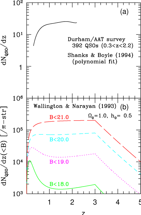
Figure 1: Redshift distribution of QSOs from (a) the Durham/AAT sample (Shanks & Boyle 1994) and that based on (b) the luminosity function by Wallington & Narayan (1993) with different B-band limiting magnitudes.

for $0.3<z<2.2$ (392 QSOs in total) which is plotted in Figure 1a. We translate the count $N(z)$ to the observed mean number density $n_{0}(r)$ according to

$$n_{0}(r)\propto{dN\over dz}{1\over r^{2}(z)}{dz\over dr},$$ (31)

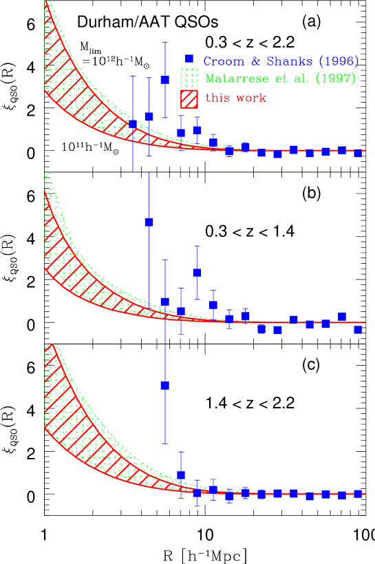
Figure 2: Two-point correlation functions of QSOs for Durham/AAT sample (Shanks & Boyle 1994; Croom & Shanks 1996) for (a) $0.3<z<2.2$, (b) $0.3<z<1.4$, and (c) $1.4<z<2.2$. Our $\xi_{A}^{\rm LC}(R)$ with $M_{\rm lim}=10^{11}$ and $10^{12}h^{-1}M_{\odot}$ are plotted in the shaded region. (Our $\xi_{B}^{\rm LC}(R)$ is almost indistinguishable from $\xi_{A}^{\rm LC}(R)$ in this case.) For comparison, the results by Matarrese et al. (1997) are plotted in the dotted hatched regions.

where the proportional constant is not necessary in our formulae. In this case we found that both equations (23) and (24) yield almost indistinguishable results. Our results are plotted in Figure 2 along with those of Matarrese et al. (1997). It is clear that the three expressions for the light-cone correlation functions result in negligible difference, at least comparing with both the statistical errors from the Durham/AAT QSO sample and the theoretical uncertainty of the evolution of bias. In the next subsection, however, we show that equations (23) and (24) exhibit significantly behavior at large $R$ where the correlation is weak. Unfortunately we are not able to make further comparison with equation (1) proposed by Matarrese et al. (1997) since we are not sure how to deal with the double integration precisely.

4.2 2dF and SDSS QSO samples

It seems premature to draw any cosmological conclusions from the comparison with the currently available data samples. Therefore we apply our formulae, $\xi_{A}^{\rm LC}(R)$ and $\xi_{B}^{\rm LC}(R)$, to predict the correlation functions for the ongoing SDSS and 2dF QSO catalogues. In this case we need a redshift dependent QSO luminosity function which is not well-established, especially at higher redshifts. In what follows we adopt the B-band quasar luminosity function according to Wallington & Narayan (1993; see also Boyle, Shanks & Peterson 1988 and Nakamura & Suto 1997). To be specific, for $0.3<z<3$

$$\Phi(M_{\rm B},z) = {\Phi_{*}\over 10^{0.4(\alpha+1)[M_{\rm B}-M_{\rm B}^{*}(z)]}+10^{0.4(\beta+1)[M_{\rm B}-M_{\rm B}^{*}(z)]}},$$ (32)

$$M_{\rm B}^{*}(z) = M_{\rm B}^{*}-2.5k_{\rm L}\log(1+z),$$ (33)

with $M_{\rm B}^{*}=-20.91+5\log h$, $k_{\rm L}=3.15$, $\alpha=-3.79$, $\beta=-1.44$, $\Phi_{*}=6.4\times 10^{-6}h^{3}{\rm Mpc}^{3}$. For $z>3$, they adopt

$$\Phi(M_{\rm B},z) = {\Phi_{*}\times 10^{-[A+0.4B(\beta+1)]}\over 10^{0.4(\alpha+1)[M_{\rm B}-M_{\rm B}^{*}(z)]}+10^{0.4(\beta+1)[M_{\rm B}-M_{\rm B}^{*}(z)]}},$$ (34)

$$M_{\rm B}^{*}(z) = M_{\rm B}^{*}-2.5k_{\rm L}\log 4+B,$$ (35)

with $A=(z-3)\log 3.2$, $B=2.5A/(\alpha-\beta)$. To compute the B-band apparent magnitude from a quasar of absolute magnitude $M_{\rm B}$ at $z$ (with the luminosity distance $d_{\rm L}(z)=(2/H_{0})(1+z-\sqrt{1+z})$ in the Einstein – de Sitter universe), we applied the K-correction:

$$B=M_{\rm B}+5\log(d_{\rm L}(z)/10{\rm pc})-2.5(1-p)\log(1+z)$$ (36)

for the quasar energy spectrum $L_{\nu}\propto\nu^{-p}$ (we use $p=0.5$). We adopt the B-band limiting magnitudes for 2dF and SDSS QSO samples as $B_{\rm lim}=20.85$ and 20, respectively. The redshift distribution of QSOs predicted from the above luminosity function is plotted in Figure 1b with the B-band limiting magnitudes $B_{\rm lim}=(18\sim 21)$.

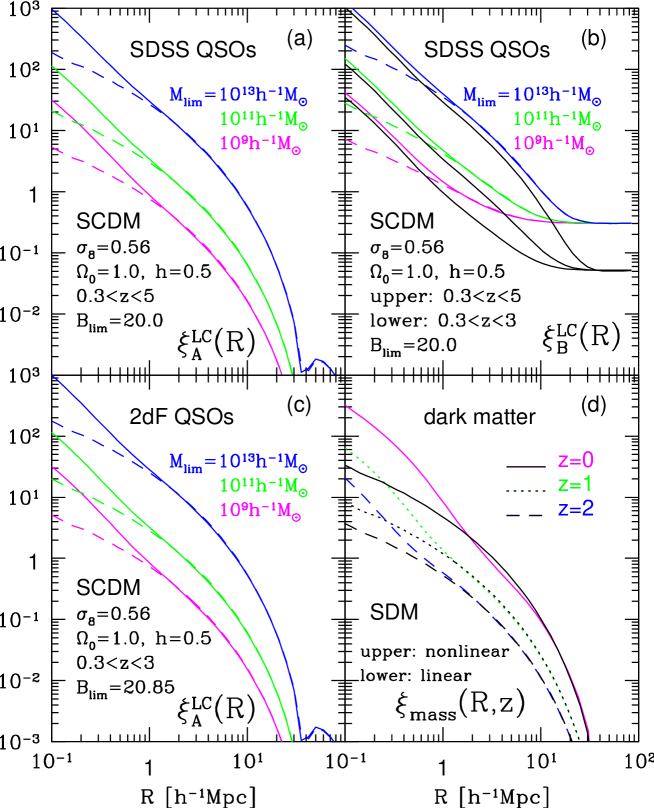
Figure 3: Two-point correlation functions of QSOs defined on the light-cone hypersurface in cluster normalized standard CDM models ($\sigma_{8}=0.56$). (a) $\xi_{A}(R)$ for the SDSS QSO catalogue for the threshold mass $M_{\rm lim}=10^{9}$, $10^{11}$ and $10^{13}h^{-1}M_{\odot}$. Nonlinear mass correlation function by Peacock & Dodds (1996) is used for solid lines, while mass correlation function in linear theory is used for dashed lines; (b) the same as (a) for $\xi_{B}(R)$; (c) the same as (a) for the 2dF QSO catalogue; (d) linear (lower curves) and nonlinear (upper curves: Peacock & Dodds 1996) mass correlation functions defined on constant-time hypersurfaces $z=0$, 1 and 2.

We show our $\xi_{A}^{\rm LC}(R)$ and $\xi_{B}^{\rm LC}(R)$ for SDSS and 2dF QSO samples together with the nonlinear mass two-point correlation functions in Figure 3. Here we adopt the standard cold dark matter (SCDM) model, in which $\Omega_{0}=1$, $\lambda=0.0$, $h=0.5$, and the amplitude of the CDM density power spectrum is normalized as $\sigma_{8}=0.56$ according to the cluster abundances (e.g., Kitayama & Suto 1996). Three lines correspond to different threshold mass $M_{\rm lim}=10^{13}$, $10^{11}$ and $10^{9}M_{\odot}$ (from top to bottom) of the dark matter halos which are supposed to host each QSO (Matarrese et al. 1997).

We plot the results using the linear fluctuation power spectrum in dashed lines while solid lines use the non-linear models of Peacock & Dodds (1996). The nonlinearity becomes important only on $R\lower 2.15277pt\hbox{$\;\buildrel<\over{\sim}\;$}1{\hbox{$h^{-1}$}{\rm Mpc}}$ implying that one can safely ignore the nonlinear effect on scales which are probed by (sparse) QSO samples in general. The linear and nonlinear correlation functions for dark matter (defined on the constant-time hypersurface) are plotted in Figure 3d.

Panels (a) and (b) adopt the B-band limiting magnitude $B_{\rm lim}=20.0$ corresponding to the SDSS QSO catalogue, while panel (c) adopts $B_{\rm lim}=20.85$ for the 2dF QSO catalogue. In practice, those two predictions are very similar if we use $\xi_{A}^{\rm LC}(R)$. On the other hand, $\xi_{B}^{\rm LC}(R)$ behaves quite differently; in fact it levels off at large $R$, and the asymptotic value depends on the range of $z$ (Fig.3b). This is qualitatively explained as follows; since ${\cal W}(R)$ decreases as $R$ and ${\cal U}(R)$ is independent of $R$ at large $R$, equations (18) and (24) imply that $\xi_{B}^{\rm LC}(R)$ becomes asymptotically

$$\lim_{R\rightarrow\infty}\xi_{B}^{\rm LC}(R)={{\cal U}(R)-\bigl{<}{\bar{n}^{\rm LC}}\bigr{>}^{2}\over\bigl{<}{\bar{n}^{\rm LC}}\bigr{>}^{2}}={{\displaystyle\int_{r_{\rm min}}^{r_{\rm max}}r^{2}dr\times\int_{r_{\rm min}}^{r_{\rm max}}r^{2}dr[n_{0}(\eta_{0}-r)]^{2}}\over{\displaystyle\left[\int_{r_{\rm min}}^{r_{\rm max}}r^{2}drn_{0}(\eta_{0}-r)\right]^{2}}}-1.$$ (37)

The right-hand side of the above equation does not vanish unless $n_{0}(\eta)$ is constant, and becomes larger as $n_{0}(\eta)$ changes more significantly within the survey volume. This is why $\xi_{B}^{\rm LC}(R)$ becomes significantly different from $\xi_{A}^{\rm LC}(R)$ when the survey limit exceeds $z\sim 3$ where the QSO number density begins to decrease substantially (see Fig. 1a and b). Incidentally this feature was not clear in Figure 2 because the Durham/AAT QSO sample is limited to $z<2.2$ and also because the Figure is plotted in linear, not log, scale.

This clearly illustrates the fact that the spatial clustering of objects defined on the light-cone could be apparently contaminated and mixed up with the intrinsic evolution of mean density of objects and even with the shape of observational selection function. In this respect, our proposal of $\xi^{\rm LC}_{A}(R)$ is a more reliable and robust definition describing the two-point correlation on the light-cone.

4.3 dependence on the cosmological model parameters

The next important question is the extent to which different cosmological models lead to different predictions of two-point correlations. For this study, we need the QSO luminosity function and bias models for the arbitrary cosmological models which are not available at this point. So we simply adopt the Durham/AAT QSO redshift distribution function (30) and the bias model (29), although the latter is derived in the Einstein – de Sitter universe.

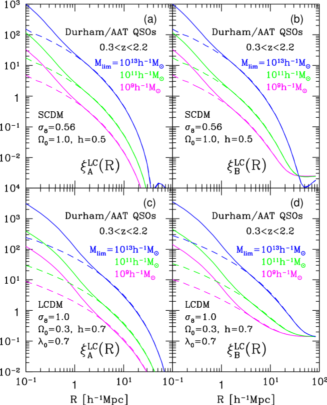
Figure 4: Dependence on the cosmological models. (a) $\xi_{A}(R)$ for the SCDM model $(\Omega_{0}=1,~{}h=0.5,~{}\sigma_{8}=0.56)$ of QSO for Durham/AAT sample (Shanks & Boyle 1994; Croom & Shanks 1996). Our $\xi_{A}^{\rm LC}(R)$ with $M_{\rm lim}=10^{9}$, $10^{11}$, and $10^{13}h^{-1}M_{\odot}$ for bias model are plotted. Nonlinear mass correlation function by Peacock & Dodds (1996) is used for solid lines, while its linear theory counterpart is used for dashed lines; (b) the same as (a) for $\xi_{B}(R)$; (c) the same as (a) for LCDM model $(\Omega_{0}=0.3,~{}\lambda_{0}=0.7,~{}~{}h=0.7,~{}\sigma_{8}=1.0)$; (d) the same as (c) for $\xi_{B}(R)$.

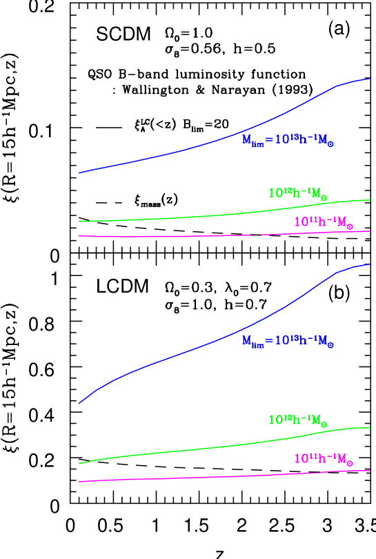
Figure 5: Evolution of amplitudes of two-point correlation functions at $R=15{\hbox{$h^{-1}$}{\rm Mpc}}$ of QSOs on the light-cone in (a) SCDM, and (b) LCDM models.

In Figure 4, we compare the predictions in the SCDM model against those in the spatially-flat low-density CDM (LCDM) model in which $\Omega_{0}=0.3$, $\lambda=0.7$, $h=0.7$, and $\sigma_{8}=1.0$. Figure 5 plots the amplitude of $\xi^{\rm LC}_{A}(R)$ at $R=15h^{-1}$Mpc as a function of the redshift of the survey limit while keeping $B_{\rm lim}=20$. Since LCDM has more power on larger scales and the fluctuation amplitude $\sigma_{8}$ is larger, the correlation is stronger compared with that in SCDM given the same bias model. It should be noted that either model predicts that the QSO correlation amplitude increases as $z$ becomes larger unlike the mass correlation which always grows from high to low redshifts. This qualitative feature is consistent with the finding of La Franca, Andreani & Cristiani (1998), and implies that the evolution of bias dominates the growth of high-z objects in addition to the growth rate of the mass fluctuations. Therefore this kind of comparison should yield profound cosmological implications on the nature of QSOs, although it would be premature to draw any decisive conclusion with the current theoretical understanding of the bias (e.g., Fry 1996; Mo & White 1996; Mo. Jing, & White 1997; Fang & Jing 1998; Jing 1998) and statistics of the observational samples.

5 Discussion and conclusions

Although the clustering of objects at high redshifts has been extensively discussed in the literature, the previous theoretical analysis was largely based on a more or less qualitative treatment of the light-cone effect (Matarrese et al. 1997; Matsubara, Suto & Szapudi 1997; Nakamura, Matsubara & Suto 1998). For on-going wide and deep surveys like SDSS and 2dF QSO surveys, the light-cone effect becomes very important either as a contamination of the real signal or as a cosmological probe.

In the present paper, we developed a theoretical formulation which properly takes account of the light-cone effect for the first time. Strictly speaking we were able to derive our main result, equation (15), only in linear theory, but we expect that the same expression would be a good approximation even in nonlinear regime. In any case the correlations of objects at high redshifts are described almost entirely in linear theory for $R\lower 2.15277pt\hbox{$\;\buildrel>\over{\sim}\;$}1{\hbox{$h^{-1}$}{\rm Mpc}}$ (Figs.3 and 4), and in practice the expression is guaranteed to be valid on the scales of interest.

We proposed a well-defined expression, equation (23), for two-point correlation functions on light-cone, and compared its implications with those of another possibility (24). As long as the Durham/AAT QSO sample is considered, both expressions give almost indistinguishable results and in fact they are also in good agreement with the previous proposal by Matarrese et al. (1997). Although we are not able to make further quantitative comparison with the latter, this implies that our proposal without the double integration over the redshift distribution is more practical in making theoretical predictions. Then we applied our expressions and computed the two-point correlation functions on light-cone for future SDSS and 2dF QSO samples, and showed an example that the light-cone effect could mix up the true spatial clustering of objects and the intrinsic evolution of mean density of objects if one uses a native definition like equation (24).

In fact there are several issues which remain to be worked out in the present context. The QSO luminosity function and the evolution of bias play central roles in confronting observations and predictions of the QSO correlation functions. In this paper, we tentatively adopted the expression by Wallington & Narayan (1993) even in LCDM models, although it is relevant only in the Einstein - de Sitter model. It is highly desirable that the QSO luminosity function in general cosmological models is derived from future observations and becomes available for the theoretical analysis. Theoretical approaches to determine the time (and scale) dependence of bias are just in the beginning (Fry 1996; Mo & White 1996; Jing 1998; Dekel & Lahav 1999). We did not attempt to explore a range of possible bias models, but rather adopt a simple fit by Matarrese et al. (1997) as a specific example. Most likely QSO correlation functions from future samples are the most straightforward tool to test the several bias models in further detail. In the present paper, we have neglected the redshift-space distortion either to the peculiar velocity of the objects (Kaiser 1987; Hamilton 1997; Nishioka & Yamamoto 1999) or to the geometry of the universe (Matsubara & Suto 1996; Ballinger, Peacock & Heavens 1996). Definitely these effects should be crucial in the quantitative comparison to high precision, and we plan to incorporate the effect in future work. Nevertheless we hope that the current paper presents a convincing case that the light-cone effect should be properly taken into account in analysing the future surveys of high-redshifts objects.

We deeply thank Sabino Matarrese and Lauro Moscardini for providing us their results in a computer readable form and also for useful correspondences on the formulation of two-point correlation functions on the light-cone. We are also grateful to Scott Croom and Tom Shanks for allowing us to include their correlation data in Figure 2, Y.P. Jing for providing the routines to compute the nonlinear mass two-point correlation functions, and to Takahiro T. Nakamura for discussions on the quasar luminosity function. We thank the referees, Richard Ellis and Stephen Landy, for constructive comments on the earlier manuscript which helped improve the presentation of the present paper. K.Y. thanks Yasufumi Kojima for comments. This research was supported in part by the Grants-in-Aid by the Ministry of Education, Science, Sports and Culture of Japan (09740203) and (07CE2002) to RESCEU.

REFERENCES

Ballinger, W.E., Peacock, J.A., & Heavens, A.F. 1996, MNRAS, 282, 877

Boyle, B.J., Croom, S.M., Smith, R.J., Shanks, T., Miller L., & Loaring, N. 1998, Phil.Trans.R.Soc.Lond.A, in press (astro-ph/9805140).

Boyle, B.J., Shanks, T., & Peterson, B.A. 1988, MNRAS, 235, 935

Carrera, F.J. et al. 1998, MNRAS, 299, 229

Croom, S.M. & Shanks, T. 1996, MNRAS, 281, 893

Dekel, A. & Lahav, O. 1999, ApJ, in press (astro-ph/9806193).

Fang, L.Z. & Jing, Y.P. 1998, ApJ, 502, L95

Fry, J. N. 1996, ApJ, 461, L65

Garnavich, P.M. et al. 1998, ApJ, 493, L53

Hamilton, A.J.S. 1997, to appear in the Proceedings of Ringberg Workshop on Large-Scale Structure, edited by Hamilton, D. (astro-ph/9708102).

Hamilton, A.J.S., Kumar, P., Lu, E., & Matthews, A. 1991, ApJ, 374, L1

Jain, B., Mo, H.J., & White, S.D.M. 1995, MNRAS, 276, L25

Jing, Y.P. 1998, ApJ, 503, L9

Jing, Y.P., & Suto, Y. 1998, ApJ, 494, L5

Kaiser, N. 1987, MNRAS, 227, 1

Kitayama, T., Sasaki,S., & Suto, Y. 1998, PASJ, 50, 1

Kitayama, T. & Suto, Y. 1997, ApJ, 490, 557

La Franca, F., Andreani, P., & Cristiani, S. 1998, ApJ, 497, 529

Lahav, O., Piran,T., & Treyer, M. 1997, MNRAS, 284, 499

Magliocchetti. M., Maddox, S.J., Lahav, O., & Wall, J.V 1998, MNRAS, 300, 257

Magnus, W., Oberhettinger, F., & Soni, R.P. 1966, Formulas and Theorems for the Special Functions of Mathematical Physics (Springer-Verlag: Berlin)

Matarrese, S., Coles, P., Lucchin, F., & Moscardini, L. 1997, MNRAS, 286, 115

Matsubara, T. & Suto, Y. 1996, ApJ, 470, L1

Matsubara, T. , Suto, Y., & Szapudi 1997, ApJ, 491, L1

Mo, H.J., Jing, Y.P., & White, S.D.M. 1997, MNRAS, 284, 189

Mo, H.J., & White, S.D.M. 1996, MNRAS, 282, 347

Nakamura, T.T., Matsubara, T. & Suto, Y. 1998, ApJ, 494, 13

Nakamura, T.T., & Suto, Y. 1997, Prog. Theor. Phys., 97, 49

Nishioka, H, & Yamamoto, K. 1999, ApJ submitted.

Peacock, J.A. & Dodds, S.J. 1994, MNRAS, 267, 1020

Peacock, J.A. & Dodds, S.J. 1996, MNRAS, 280, L19

Shanks, T. & Boyle, B.J. 1994, MNRAS, 271, 753

Steidel, C.C., Adelberger, K.L., Dickinson, M., Giavalisco, M., Pettini, M., & Kellogg, M. 1998, ApJ, 492, 428

Wallington, S., & Narayan, R. 1993, ApJ, 403, 517

Yamamoto, K., & Sugiyama, N. 1998, Phys.Rev.D 58, 103508.

Yamamoto, K., & Suto, Y. 1999, in preparation.

Appendices

Appendix A Calculation of ${\cal W}(R)$

We present an explicit derivation of equation (12) from equation (11):

$${\cal W}(R)={1\over V^{\rm LC}}\int{d\Omega_{\hat{\bf R}}\over 4\pi}\int dr_{1}r_{1}^{2}\int d\Omega_{{\vec{\gamma}}_{1}}\int dr_{2}r_{2}^{2}\int d\Omega_{{\vec{\gamma}}_{2}}n_{0}(\eta_{0}-r_{1})n_{0}(\eta_{0}-r_{2})$$

$$\hskip 42.67912pt\times\Bigl{<}\Delta(\eta_{0}-r_{1},r_{1},{\vec{\gamma}}_{1})\Delta(\eta_{0}-r_{2},r_{2},{\vec{\gamma}}_{2})\Bigr{>}\delta^{(3)}({\bf x}_{1}-{\bf x}_{2}-{\bf R})$$ (A1)

in linear theory.

First let us expand the number density contrast $\Delta(\eta,r,{\vec{\gamma}})$ as

$$\Delta(\eta,r,{\vec{\gamma}})=\int_{0}^{\infty}dk\sum_{l,m}\Delta_{klm}(\eta){\cal Y}_{klm}(r,{\vec{\gamma}}),$$ (A2)

in terms of the normalized harmonics:

$${\cal Y}_{klm}(r,{\vec{\gamma}})=X_{kl}(r)Y_{lm}(\Omega_{{\vec{\gamma}}}),$$ (A3)

where

$$X_{kl}(r)=\sqrt{{2\over\pi}}kj_{l}(kr),$$ (A4)

and $Y_{lm}(\Omega_{{\vec{\gamma}}})$ and $j_{l}(x)$ are the spherical harmonics and the spherical Bessel function, respectively.

Substituting equation (A2) into equation (A1), one obtains

$${\cal W}(R) = {1\over V^{\rm LC}}\int{d\Omega_{\hat{\bf R}}\over 4\pi}\int dr_{1}r_{1}^{2}\int d\Omega_{{\vec{\gamma}}_{1}}\int dr_{2}r_{2}^{2}\int d\Omega_{{\vec{\gamma}}_{2}}n_{0}(\eta_{0}-r_{1})n_{0}(\eta_{0}-r_{2})$$ (A5)

$$\times\int dk_{1}\sum_{l_{1},m_{1}}\int dk_{2}\sum_{l_{2},m_{2}}\bigl{<}\Delta_{k_{1}l_{1}m_{1}}(\eta_{0}-r_{1})\Delta_{k_{2}l_{2}m_{2}}^{*}(\eta_{0}-r_{2})\bigr{>}$$

$$\times{X}_{k_{1}l_{1}}(r_{1})Y_{l_{1}m_{1}}(\Omega_{{\vec{\gamma}}_{1}}){X}_{k_{2}l_{2}}(r_{2})Y_{l_{2}m_{2}}^{*}(\Omega_{{\vec{\gamma}}_{2}})~{}\delta^{(3)}({\bf x}_{1}-{\bf x}_{2}-{\bf R}).$$

In Appendix B, we show that the ensemble average of the mode coefficient in the integrand of equation (A5) reduces to the following function:

$$\bigl{<}\Delta_{k_{1}l_{1}m_{1}}(\eta_{0}-r_{1})\Delta_{k_{2}l_{2}m_{2}}^{*}(\eta_{0}-r_{2})\bigr{>}=Q(k_{1},k_{2},r_{1},r_{2},l_{1})\delta_{l_{1}l_{2}}\delta_{m_{1}m_{2}},$$ (A6)

where $\delta_{l_{1}l_{2}}$ and $\delta_{m_{1}m_{2}}$ are the Kronecker’s delta. In addition, we use the relations

$$\delta^{(3)}({\bf x}_{1}-{\bf x}_{2}-{\bf R})={1\over(2\pi)^{3}}\int d^{3}{\bf k}~{}e^{-i{\bf k}\cdot({\bf x}_{1}-{\bf x}_{2}-{\bf R})},$$ (A7)

and

$$e^{-i{\bf k}\cdot{\bf x}}=4\pi\sum_{l}\sum_{m=-l}^{l}(-i)^{l}j_{l}(k|{\bf x}|)Y_{lm}(\Omega_{\hat{\bf k}})Y_{lm}^{*}(\Omega_{\hat{\bf x}}),$$ (A8)

and then equation (A5) becomes

$${\cal W}(R) = {1\over V^{\rm LC}}\int{d\Omega_{\hat{\bf R}}\over 4\pi}\int dr_{1}r_{1}^{2}\int d\Omega_{{\vec{\gamma}}_{1}}\int dr_{2}r_{2}^{2}\int d\Omega_{{\vec{\gamma}}_{2}}n_{0}(\eta_{0}-r_{1})n_{0}(\eta_{0}-r_{2})$$ (A9)

$$\times\int dk_{1}\sum_{l_{1},m_{1}}\int dk_{2}\sum_{l_{2},m_{2}}Q(k_{1},k_{2},r_{1},r_{2},l_{1})\delta_{l_{1}l_{2}}\delta_{m_{1}m_{2}}$$

$$\times{X}_{k_{1}l_{1}}(r_{1})Y_{l_{1}m_{1}}(\Omega_{{\vec{\gamma}}_{1}}){X}_{k_{2}l_{2}}(r_{2})Y_{l_{2}m_{2}}^{*}(\Omega_{{\vec{\gamma}}_{2}})~{}$$

$$\times{1\over(2\pi)^{3}}\int d^{3}{\bf k}~{}4\pi\sum_{L_{1}M_{1}}(-i)^{L_{1}}j_{L_{1}}(kr_{1})Y_{L_{1}M_{1}}(\Omega_{\hat{\bf k}})Y_{L_{1}M_{1}}^{*}(\Omega_{{\vec{\gamma}}_{1}})$$

$$\hskip 65.44142pt\times 4\pi\sum_{L_{2}M_{2}}(i)^{L_{2}}j_{L_{2}}(kr_{2})Y_{L_{2}M_{2}}^{*}(\Omega_{\hat{\bf k}})Y_{L_{2}M_{2}}(\Omega_{{\vec{\gamma}}_{2}})$$

$$\hskip 65.44142pt\times 4\pi\sum_{L_{3}M_{3}}(i)^{L_{3}}j_{L_{3}}(kR)Y_{L_{3}M_{3}}^{*}(\Omega_{\hat{\bf k}})Y_{L_{3}M_{3}}(\Omega_{\hat{\bf R}})~{},$$

where $k=|{\bf k}|$ and $\hat{\bf k}={\bf k}/|{\bf k}|$. Integrating over $\Omega_{{\vec{\gamma}}_{1}}$, $\Omega_{{\vec{\gamma}}_{2}}$ and $\Omega_{{\hat{\bf R}}}$ yields

$${\cal W}(R) = {1\over V^{\rm LC}}\int dr_{1}r_{1}^{2}\int dr_{2}r_{2}^{2}n_{0}(\eta_{0}-r_{1})n_{0}(\eta_{0}-r_{2})$$ (A10)

$$\times\int dk_{1}\sum_{l_{1},m_{1}}\int dk_{2}\sum_{l_{2},m_{2}}Q(k_{1},k_{2},r_{1},r_{2},l_{1})\delta_{l_{1}l_{2}}\delta_{m_{1}m_{2}}{X}_{k_{1}l_{1}}(r_{1}){X}_{k_{2}l_{2}}(r_{2})$$

$$\times{(4\pi)^{2}\over(2\pi)^{3}}\int d^{3}{\bf k}(-i)^{l_{1}-l_{2}}j_{l_{1}}(kr_{1})j_{l_{2}}(kr_{2})j_{0}(kR)Y_{l_{1}m_{1}}(\Omega_{\hat{\bf k}})Y_{l_{2}m_{2}}^{*}(\Omega_{\hat{\bf k}}).$$

and the further integration over $\Omega_{\hat{{\bf k}}}$ gives

$${\cal W}(R) = {1\over V^{\rm LC}}\int dr_{1}r_{1}^{2}\int dr_{2}r_{2}^{2}n_{0}(\eta_{0}-r_{1})n_{0}(\eta_{0}-r_{2})$$ (A11)

$$\times\int dk_{1}\int dk_{2}\sum_{l}(2l+1)Q(k_{1},k_{2},r_{1},r_{2},l){X}_{k_{1}l}(r_{1}){X}_{k_{2}l}(r_{2})$$

$$\times{(4\pi)^{2}\over(2\pi)^{3}}\int dkk^{2}j_{l}(kr_{1})j_{l}(kr_{2})j_{0}(kR).$$

Noting the relation (e.g., Magnus et al. 1966):

$$\int dkk^{2}j_{l}(kr_{1})j_{l}(kr_{2})j_{0}(kR)=\left\{\begin{array}[]{ll}{\pi\over 4r_{1}r_{2}R}P_{l}\biggl{(}{r_{1}^{2}+r_{2}^{2}-R^{2}\over 2r_{1}r_{2}}\biggr{)}&\mbox{($|r_{1}-r_{2}|<R<r_{1}+r_{2}$)},\\ 0&\mbox{($R<|r_{1}-r_{2}|$, $R>r_{1}+r_{2}$)},\end{array}\right.$$ (A14)

we find

$${\cal W}(R)={1\over V^{\rm LC}}{1\over\pi R}\int\int_{\cal S}dr_{1}dr_{2}r_{1}r_{2}n_{0}(\eta_{0}-r_{1})n_{0}(\eta_{0}-r_{2})\int dk_{1}\int dk_{2}k_{1}k_{2}$$

$$\hskip 28.45274pt\times\sum_{l}(2l+1)Q(k_{1},k_{2},r_{1},r_{2},l)j_{l}(k_{1}r_{1})j_{l}(k_{2}r_{2})P_{l}\biggl{(}{r_{1}^{2}+r_{2}^{2}-R^{2}\over 2r_{1}r_{2}}\biggr{)},$$ (A15)

where $\cal S$ denotes the region $|r_{1}-r_{2}|\leq R\leq r_{1}+r_{2}$.

So far we did not assume anything on the density field, i.e., $Q(k_{1},k_{2},r_{1},r_{2},l)$ can be an arbitrary function. If we consider the case of linear theory and a scale-dependent but still local biasing scheme, each mode is decoupled and we can write

$$Q(k_{1},k_{2},r_{1},r_{2},l)=D_{1}(\eta_{0}-r_{1})D_{1}(\eta_{0}-r_{2})b(k_{1};\eta_{0}-r_{1})b(k_{2};\eta_{0}-r_{2})P(k)\delta(k_{1}-k_{2}),$$ (A16)

where $D_{1}(\eta)$ is the linear growth rate normalized to unity at present and $b(k;\eta)$ is the scale-dependent bias factor. In this case, equation (A15) is written as

$${\cal W}(R)={1\over V^{\rm LC}}{1\over\pi R}\int\int_{\cal S}dr_{1}dr_{2}\prod_{j=1}^{2}\biggl{(}r_{j}n_{0}(\eta_{0}-r_{j})D_{1}(\eta_{0}-r_{j})\biggr{)}$$

$$\hskip 28.45274pt\times\int dkk^{2}P(k)b(k;\eta_{0}-r_{1})b(k;\eta_{0}-r_{2})$$

$$\hskip 28.45274pt\times\sum_{l}(2l+1)j_{l}(kr_{1})j_{l}(kr_{2})P_{l}\biggl{(}{r_{1}^{2}+r_{2}^{2}-R^{2}\over 2r_{1}r_{2}}\biggr{)}.$$ (A17)

Using the formula:

$$\sum_{l}(2l+1)j_{l}(kr_{1})j_{l}(kr_{2})P_{l}\biggl{(}{r_{1}^{2}+r_{2}^{2}-R^{2}\over 2r_{1}r_{2}}\biggr{)}=j_{0}(kR),$$ (A18)

we finally obtain

$${\cal W}(R) = {1\over V^{\rm LC}}{1\over\pi R}\int\int_{\cal S}dr_{1}dr_{2}r_{1}r_{2}\prod_{j=1}^{2}\biggl{(}n_{0}(\eta_{0}-r_{j})D_{1}(\eta_{0}-r_{j})\biggr{)}$$ (A19)

$$\times\int dkk^{2}P(k)j_{0}(kR)b(k;\eta_{0}-r_{1})b(k;\eta_{0}-r_{2}),$$

which is identical to equation (12).

Appendix B The power spectrum of mode coefficients

Here we derive equation (A6) which is used in Appendix A. Since equation (A2) implies that the mode coefficient $\Delta_{klm}(\eta)$ is expressed as

$$\Delta_{klm}(\eta)=\int drr^{2}d\Omega_{{\vec{\gamma}}}\Delta(\eta,r,{\vec{\gamma}}){\cal Y}_{klm}(r,{\vec{\gamma}}),$$ (B1)

one obtains

$$\bigl{<}\Delta_{k_{1}l_{1}m_{1}}(\eta_{1})\Delta_{k_{2}l_{2}m_{2}}^{*}(\eta_{2})\bigr{>}=\int dr_{1}r_{1}^{2}d\Omega_{{\vec{\gamma}}_{1}}\int dr_{2}r_{2}^{2}d\Omega_{{\vec{\gamma}}_{2}}$$

$$\hskip 56.9055pt\times\bigl{<}\Delta(\eta_{1},r_{1},{\vec{\gamma}}_{1})\Delta(\eta_{2},r_{2},{\vec{\gamma}}_{2})\bigr{>}{\cal Y}_{k_{1}l_{1}m_{1}}(r_{1},{\vec{\gamma}}_{1}){\cal Y}^{*}_{k_{2}l_{2}m_{2}}(r_{2},{\vec{\gamma}}_{2}).$$ (B2)

Since the correlation on the light-cone hypersurface does not have any special direction in ${\vec{\gamma}}$, the ensemble average $\bigl{<}\Delta(\eta_{1},r_{1},{\vec{\gamma}}_{1})\Delta(\eta_{2},r_{2},{\vec{\gamma}}_{2})\bigr{>}$ should be a function of $\eta_{1}$, $\eta_{2}$, $r_{1}$, $r_{2}$ and $\cos\theta(\equiv{\vec{\gamma}}_{1}\cdot{\vec{\gamma}}_{2})$:

$$\bigl{<}\Delta(\eta_{1},r_{1},{\vec{\gamma}}_{1})\Delta(\eta_{2},r_{2},{\vec{\gamma}}_{2})\bigr{>}=F(\eta_{1},\eta_{2},r_{1},r_{2},\cos\theta).$$ (B3)

The function in the right-hand side of the above equation can be expanded in general as

$$F(\eta_{1},\eta_{2},r_{1},r_{2},\cos\theta) = \sum_{l}{2l+1\over 4\pi}C(\eta_{1},\eta_{2},r_{1},r_{2},l)P_{l}(\cos\theta)$$ (B4)

$$= \sum_{l}\sum_{m=-l}^{l}C(\eta_{1},\eta_{2},r_{1},r_{2},l)Y^{*}_{lm}(\Omega_{{\vec{\gamma}}_{1}})Y_{lm}(\Omega_{{\vec{\gamma}}_{2}}).$$

Substituting the above expansion into equation (B2) and integrating over $d\Omega_{{\vec{\gamma}}_{1}}$ and $d\Omega_{{\vec{\gamma}}_{2}}$, we obtain equation (A6):

$$\bigl{<}\Delta_{k_{1}l_{1}m_{1}}(\eta_{1})\Delta_{k_{2}l_{2}m_{2}}^{*}(\eta_{2})\bigr{>}=Q(k_{1},k_{2},\eta_{1},\eta_{2},l_{1})\delta_{l_{1}l_{2}}\delta_{m_{1}m_{2}},$$ (B5)

where

$$Q(k_{1},k_{2},\eta_{1},\eta_{2},l)=\int r_{1}^{2}dr_{1}\int r_{2}^{2}dr_{2}C(\eta_{1},\eta_{2},r_{1},r_{2},l)X_{k_{1}l}(r_{1})X_{k_{2}l}(r_{2}).$$ (B6)