Streaming velocities as a dynamical estimator of $\Omega$

Abstract

It is well known that estimating the mean pairwise velocity of galaxies, ${v_{{\scriptscriptstyle 12}}}$, from the redshift space galaxy correlation function is difficult because this method is highly sensitive to the assumed model of the pairwise velocity dispersion. Here we propose an alternative method to estimate ${v_{{\scriptscriptstyle 12}}}$ directly from peculiar velocity samples, which contain redshift-independent distances as well as galaxy redshifts. In contrast to other dynamical measures which determine $\beta\equiv\Omega^{0.6}{\sigma_{{\scriptscriptstyle 8}}}$, this method can provide an estimate of $\Omega^{0.6}{\sigma_{{\scriptscriptstyle 8}}}^{2}$ for a range of ${\sigma_{{\scriptscriptstyle 8}}}$ where $\Omega$ is the cosmological density parameter, while ${\sigma_{{\scriptscriptstyle 8}}}$ is the standard normalization for the power spectrum of density fluctuations. We demonstrate how to measure this quantity from realistic catalogues.

1 Introduction

In this Letter we investigate the possibility of using the “mean tendency of well-separated galaxies to approach each other” (Peebles 1980, hereafter LSS) to measure the cosmological density parameter, $\Omega$. The statistic we consider is the mean relative pairwise velocity of galaxies, ${v_{{\scriptscriptstyle 12}}}$. It was introduced in the context of the BBGKY theory (Davis and Peebles 1977), describing the dynamical evolution of a collection of particles interacting through gravity. In this discrete picture, ${{\vec{v}}_{{\scriptscriptstyle 12}}}$ is defined as the mean value of the peculiar velocity difference of a particle pair at separation ${\vec{r}}$ (LSS, Eq. 71.4). In the fluid limit, its analogue is the pair-density weighted relative velocity (Fisher et al. (1994); Juszkiewicz et al. 1998a ),

$${{\vec{v}}_{{\scriptscriptstyle 12}}}(r)\;=\;\langle\,{{\vec{v}}_{{\scriptscriptstyle 1}}}-{{\vec{v}}_{{\scriptscriptstyle 2}}}\,\rangle_{\scriptscriptstyle{\rho}}\;=\;{{\langle({{\vec{v}}_{{\scriptscriptstyle 1}}}-{{\vec{v}}_{{\scriptscriptstyle 2}}})(1+{{\delta}_{{\scriptscriptstyle 1}}})(1+{{\delta}_{{\scriptscriptstyle 2}}})\rangle}\over{1\;+\;\xi(r)}}\;,$$ (1)

where $\,{{\vec{v}}_{{\scriptscriptstyle A}}}\,$ and $\,{{\delta}_{{\scriptscriptstyle A}}}={{\rho}_{{\scriptscriptstyle A}}}/\langle\rho\rangle-1\,$ are the peculiar velocity and fractional density contrast of matter at a point ${{{\vec{r}}}_{{\scriptscriptstyle A}}}$, $r=|{{\vec{r}}_{{\scriptscriptstyle 1}}}-{{\vec{r}}_{{\scriptscriptstyle 2}}}|$, and $\xi(r)=\langle{{\delta}_{{\scriptscriptstyle 1}}}{{\delta}_{{\scriptscriptstyle 2}}}\rangle$ is the two-point correlation function. The pair-weighted average, $\langle\cdots\rangle_{\scriptscriptstyle{\rho}}$, differs from simple spatial averaging, $\langle\cdots\rangle$, by the weighting factor ${{\rho}_{{\scriptscriptstyle 1}}}{{\rho}_{{\scriptscriptstyle 2}}}\,\langle{{\rho}_{{\scriptscriptstyle 1}}}{{\rho}_{{\scriptscriptstyle 2}}}\rangle^{-1}$, proportional to the number-density of particle pairs. In gravitational instability theory, the magnitude of ${{\vec{v}}_{{\scriptscriptstyle 12}}}(r)$ is related to the two point correlation function, $\xi(r)$, through the pair conservation equation (LSS, Eq. 71.6). For models with Gaussian initial conditions, the solution of the pair conservation equation is well approximated by (Juszkiewicz et al. 1998b )

$${v_{{\scriptscriptstyle 12}}}(r)\; = \;-\,{\textstyle{2\over 3}}\,Hrf\,\bar{\bar{\xi}}(r)[1+\alpha\;\bar{\bar{\xi}}(r)]\;,$$ (2)

$$\bar{\xi}(r)\; = \;(3/r^{3})\,\int_{0}^{r}\,\xi(x)\,x^{2}\,dx\;\equiv\;\bar{\bar{\xi}}(r)\,[\,1+\xi(r)\,]$$ (3)

Here $\alpha$ is a parameter, which depends on the logarithmic slope of $\xi(r)$, while $f=d\,\ln D/d\ln a$, with $D(a)$ being the standard linear growing mode solution and $a$ – the cosmological expansion factor (see e.g., LSS, §11). Finally, $H=100\;h\;\mbox{km}\;\mbox{s}^{-1}\;\mbox{Mpc}$ is the present value of the Hubble constant. For a wide class of cosmological models, including those with non-zero cosmological constant, $f\approx\Omega^{0.6}$ (Peebles (1993), hereafter PPC, §13). If $\xi\propto r^{-\gamma}$, and $\gamma$ is scale-independent, the predicted streaming velocity can be expressed in terms of $\Omega$ and the standard normalization parameter, ${\sigma_{{\scriptscriptstyle 8}}}$ – the rms matter density contrast in a ball of radius $8h^{-1}\;\mbox{Mpc}$. For a pure power-law $\xi(r)$, we have (PPC, Eq. 7.72)

$$\bar{\xi}(r)\;=\;3\,\xi(r)\,/\,(3-\gamma)\;=\;{\sigma_{{\scriptscriptstyle 8}}}^{2}(16\;h^{-1}\;\mbox{Mpc}/r)^{\gamma}(4-\gamma)(6-\gamma)/24\;.$$ (4)

For $0<\gamma<3$, the parameter $\alpha$ is given by (Juszkiewicz et al. 1998b )

$$\alpha\;\approx\;1.2\;-\;0.65\,\gamma\;.$$ (5)

The approximate solution of the pair conservation equation, given by equations (2) - (5) accurately reproduces results of high resolution N-body simulations in the entire dynamical range (Juszkiewicz et al. 1998b ). This approximate solution was designed to reproduce the second-order Eulerian perturbation theory solution in the weakly nonlinear regime ($\,|\xi|<1\,$) and the stable clustering solution in the strongly nonlinear regime $(\,\xi\gg 1,\;\;{v_{{\scriptscriptstyle 12}}}(r)=-Hr\,$; see Scoccimarro & Frieman (1996) and Łokas et al. (1996) for the second-order correction for $\xi$ and LSS, §71 for the stable clustering).

To get a better idea of how the Equation (2) can be used to estimate $\Omega$, let us consider a numerical example: ${v_{{\scriptscriptstyle 12}}}$ at a separation $\,r=10h^{-1}\,\mbox{Mpc}\,$. One can use the APM catalogue of galaxies (Efstathiou 1996) for an estimate of $\gamma$. The slope at the separation considered is $\gamma=1.75\pm 0.1$ (the errors we quote are conservative). Substituting Eqs. 4 and 5 into Eq. 2, and setting $\gamma=1.75$, we get

$${v_{{\scriptscriptstyle 12}}}(10h^{-1}\;\mbox{Mpc})\;=\;-\,605\,{{\sigma_{{\scriptscriptstyle 8}}}}^{2}\Omega^{0.6}\,(1+0.43{\sigma_{{\scriptscriptstyle 8}}}^{2})\,/(1+0.38{{\sigma_{{\scriptscriptstyle 8}}}}^{2})^{2}\,{\rm km/s}\;.$$ (6)

The above relation shows that at $r=10h^{-1}\;\mbox{Mpc}$, ${v_{{\scriptscriptstyle 12}}}$ is almost entirely determined by the values of two parameters: ${\sigma_{{\scriptscriptstyle 8}}}$ and $\Omega$. It is only weakly dependent on $\gamma$. This dependence is caused by the $\alpha\;\bar{\bar{\xi}}$ term in Eq. 2. However, for all realistic values of $\gamma$, $\alpha$ is a small number. The uncertainties in the observed $\gamma$ lead to an error in Eq. 6 of less than $10\%$ for ${\sigma_{{\scriptscriptstyle 8}}}\leq 1$.

The approximate solution, given by Equation 2 accurately reproduces ${v_{{\scriptscriptstyle 12}}}(r)$ curves for dark matter particles, measured from high resolution N-body simulations (Juszkiewicz et al. 1998b ). Moreover, Eq. 2 agrees well with measurements of mean streaming velocities of “galaxies”, $\,{v_{{\scriptscriptstyle 12g}}}(r)\,$, obtained in recent simulations, which attempt to take into account non-gravitational processes like star formation and radiative cooling (Kaufmann et al. (1998)). These simulations exhibit clustering bias, but no velocity bias ($\,{v_{{\scriptscriptstyle 12g}}}={v_{{\scriptscriptstyle 12}}}\,$), suggesting that galaxies constitute reliable test particles, driven by the gravitational field of the true mass distribution even if the galaxies themselves are biased tracers of mass.

2 The estimator

Since we observe only the line-of-sight component of the peculiar velocity, ${s_{{\scriptscriptstyle A}}}={{{\vec{r}}}_{{\scriptscriptstyle A}}}\cdot{{\vec{v}}_{{\scriptscriptstyle A}}}/r\equiv{{\hat{r}}_{{\scriptscriptstyle A}}}\cdot{{\vec{v}}_{{\scriptscriptstyle A}}}$, rather than the full three-dimensional velocity ${{\vec{v}}_{{\scriptscriptstyle A}}}$, it is not possible to compute ${v_{{\scriptscriptstyle 12}}}$ directly. Instead, we propose to use the mean difference between radial velocities of a pair of galaxies, $\langle\,{s_{{\scriptscriptstyle 1}}}-{s_{{\scriptscriptstyle 2}}}\,\rangle_{\scriptscriptstyle{\rho}}\;=\;{v_{{\scriptscriptstyle 12}}}\,{\hat{r}}\cdot({{\hat{r}}_{{\scriptscriptstyle 1}}}+{{\hat{r}}_{{\scriptscriptstyle 2}}})/2$, where ${\vec{r}}={{\vec{r}}_{{\scriptscriptstyle 1}}}-{{\vec{r}}_{{\scriptscriptstyle 2}}}$. To estimate ${v_{{\scriptscriptstyle 12}}}$, we use the simplest least squares techniques, which minimizes the quantity $\chi^{2}(r)\;=\;\sum_{{{}_{{\scriptscriptstyle A,B}}}}\,\left[({s_{{\scriptscriptstyle A}}}-{s_{{\scriptscriptstyle B}}})-{p_{{\scriptscriptstyle AB}}}\,{{\tilde{v}}_{{\scriptscriptstyle 12}}}(r)/2\,\right]^{2}\;\;$, where ${p_{{\scriptscriptstyle AB}}}\equiv{\hat{r}}\cdot({{\hat{r}}_{{\scriptscriptstyle A}}}+{{\hat{r}}_{{\scriptscriptstyle B}}})$ and the sum is over all pairs at fixed separation $r=|{{{\vec{r}}}_{{\scriptscriptstyle A}}}-{{{\vec{r}}}_{{\scriptscriptstyle B}}}|$. The condition $\partial\chi^{2}/\,\partial{{\tilde{v}}_{{\scriptscriptstyle 12}}}=0$ implies

$${{\tilde{v}}_{{\scriptscriptstyle 12}}}(r)\;=\;{{2\sum\,({s_{{\scriptscriptstyle A}}}-{s_{{\scriptscriptstyle B}}})\,{p_{{\scriptscriptstyle AB}}}}\over{\sum{p_{{\scriptscriptstyle AB}}}^{2}}}\;\;.$$ (7)

This estimator is appropriate to be applied to a point process which will sample an underlying continuous distribution. The sampling is quantified in terms of the selection function, $\phi({\vec{r}})$. The continuum limit of Eq. 7 is then

$${{\tilde{v}}_{{\scriptscriptstyle 12}}}(r)=\frac{2\int d{m_{{\scriptscriptstyle 1}}}\,d{m_{{\scriptscriptstyle 2}}}\,{\Phi_{{\scriptscriptstyle 12}}}\,({s_{{\scriptscriptstyle 1}}}-{s_{{\scriptscriptstyle 2}}}){p_{{\scriptscriptstyle 12}}}}{\int d{m_{{\scriptscriptstyle 1}}}\,d{m_{{\scriptscriptstyle 2}}}\,{\Phi_{{\scriptscriptstyle 12}}}\,{p_{{\scriptscriptstyle 12}}}^{2}}\;,$$ (8)

with $d{m_{{\scriptscriptstyle A}}}={{\rho}_{{\scriptscriptstyle A}}}~{}d^{3}{{{\vec{r}}}_{{\scriptscriptstyle A}}}$, and a two-point selection function given by ${\Phi_{{\scriptscriptstyle 12}}}\;=\;\delta_{D}(|{{{\vec{r}}_{{\scriptscriptstyle 1}}}-{{\vec{r}}_{{\scriptscriptstyle 2}}}}|-r)\,\phi({{\vec{r}}_{{\scriptscriptstyle 1}}})\,\phi({{\vec{r}}_{{\scriptscriptstyle 2}}})\;$, where $\delta_{D}$ is the Dirac delta function. For ease of notation we shall denote the denominator in Eq. 8 by $W(r)$. If we take the ensemble average of Eq. 8 we find that $\langle{{\tilde{v}}_{{\scriptscriptstyle 12}}}(r)\rangle={v_{{\scriptscriptstyle 12}}}(r)$. Note that, unlike the estimators for the velocity correlation tensor proposed in Górski et al. (1989), the ensemble average of the estimator is ${v_{{\scriptscriptstyle 12}}}(r)$ independent of the selection function. For an isotropic selection function this estimator is insensitive to systematic effects such as a bulk flow, large scale shear and small scale random velocities (as one might expect from virialized objects).

To assess how useful this statistic is in practice we calculate the covariance matrix of ${{\tilde{v}}_{{\scriptscriptstyle 12}}}(r)$; this involves calculating the ensemble average, $\langle({s_{{\scriptscriptstyle 1}}}-{s_{{\scriptscriptstyle 2}}})({s_{{\scriptscriptstyle 3}}}-{s_{{\scriptscriptstyle 4}}})\rangle_{\scriptscriptstyle{\rho}}=\langle({s_{{\scriptscriptstyle 1}}}-{s_{{\scriptscriptstyle 2}}})({s_{{\scriptscriptstyle 3}}}-{s_{{\scriptscriptstyle 4}}})\rangle+$ higher order terms. Unlike most statistics, the number weighting leads to a variance which is of the same order in perturbation theory, ${\cal O}(\delta^{2})$, as the actual quantity one is trying to estimate. The covariance between estimates of the pairwise velocity at two different separations, ${{\tilde{v}}_{{\scriptscriptstyle 12}}}={{\tilde{v}}_{{\scriptscriptstyle 12}}}(r)$, and ${{\tilde{v}}_{{\scriptscriptstyle 12}}}^{\prime}={{\tilde{v}}_{{\scriptscriptstyle 12}}}(r^{\prime})$, can be expressed as

$$\langle{{\tilde{v}}_{{\scriptscriptstyle 12}}}{{\tilde{v}}_{{\scriptscriptstyle 12}}}^{\prime}\rangle-\langle{{\tilde{v}}_{{\scriptscriptstyle 12}}}\rangle\langle{{\tilde{v}}_{{\scriptscriptstyle 12}}}^{\prime}\rangle=\int d^{3}{{\vec{r}}_{{\scriptscriptstyle 1}}}d^{3}{{\vec{r}}_{{\scriptscriptstyle 2}}}\phi({{\vec{r}}_{{\scriptscriptstyle 1}}})\phi({{\vec{r}}_{{\scriptscriptstyle 2}}})\mu(r,{{\vec{r}}_{{\scriptscriptstyle 1}}})\mu(r^{\prime},{{\vec{r}}_{{\scriptscriptstyle 2}}}){{r_{{\scriptscriptstyle 1i}}}}\Psi_{ij}(r){{r_{{\scriptscriptstyle 2j}}}}\;,$$ (9)

where ${r_{{\scriptscriptstyle Aj}}}$ is the $j^{\rm th}$ cartesian component of ${{{\vec{r}}}_{{\scriptscriptstyle A}}}$ ($A=1,2;\;j=1,2,3$), while $\Psi_{ij}({\vec{r}})\,=\,\langle v_{i}(0)v_{j}({\vec{r}})\rangle$ is the velocity correlation tensor, and $\mu(r,{{\vec{r}}_{{\scriptscriptstyle 1}}})\equiv 2W^{-1}(r)\int d^{3}{{\vec{r}}_{{\scriptscriptstyle 2}}}\phi({{\vec{r}}_{{\scriptscriptstyle 2}}})\delta_{D}(|{{\vec{r}}_{{\scriptscriptstyle 2}}}-{{\vec{r}}_{{\scriptscriptstyle 1}}}|-r){p_{{\scriptscriptstyle 12}}}$. In the linear regime, $\Psi_{ij}$ can be expressed in terms of $P(k)$ — the power spectrum of density fluctuations (Górski (1988), Groth et al. (1989)), $\Psi_{ij}\,({\vec{r}})\;=\;(H_{0}^{2}f^{2}/8\pi^{3})\,\int\,d^{3}{\vec{k}}\,P(k)\,(k_{i}k_{j}/k^{4})\,\exp(i\vec{k}\cdot{\vec{r}})$. The form of the selection function will dictate the dependence of the variance on scale. As one would expect, the smaller the depth of the selection function, the larger the variance. This is illustrated in Figure 1(a,b) where we plot the mean (dotted line) and variance of ${{\tilde{v}}_{{\scriptscriptstyle 12}}}(r)$ for two COBE normalized CDM models and for a choice of two selection functions. In this Letter we shall use a selection function of the form

$$\phi(r)\;\propto\;[r(1+(r/r_{*})^{2})]^{-1}\;;\qquad r_{*}=30\;h^{-1}\mbox{Mpc}\;,$$ (10)

which we shall refer to as the “full” selection function (plotted as the solid line in Figure 1). In many cases galaxy catalogues will have a sharply decaying selection function beyond a certain scale (Strauss $\&$ Willick 95) and it is therefore useful to check the effect such a feature will have on our estimator. We shall do so by considering the selection function of Eq. 10 truncated at $r=r_{*}$. We refer to the latter as “truncated” (dashed line in Figure 1).

A very important feature of this statistic is the possible presence of non-negligible covariance between values of the estimator at different scales. The fact that the covariance depends on the velocity correlation tensor, $\Psi$, will lead to larger covariance than what one might naively expect: the larger coherence length of this quantity (as compared to either $\xi(r)$ or ${v_{{\scriptscriptstyle 12}}}(r)$) leads to a larger coherence in the covariance matrix and consequently to larger cross correlations between ${v_{{\scriptscriptstyle 12}}}$ at different scales. In Figure 1(c,d), we plot the appropriately normalized covariance, ${\rm Cov}_{n}({{\tilde{v}}_{{\scriptscriptstyle 12}}},{{\tilde{v}}_{{\scriptscriptstyle 12}}}^{\prime})=[\langle{{\tilde{v}}_{{\scriptscriptstyle 12}}}{{\tilde{v}}_{{\scriptscriptstyle 12}}}^{\prime}\rangle-\langle{{\tilde{v}}_{{\scriptscriptstyle 12}}}\rangle\langle{{\tilde{v}}_{{\scriptscriptstyle 12}}}^{\prime}\rangle]/\sqrt{\langle{{\tilde{v}}_{{\scriptscriptstyle 12}}}^{2}\rangle\langle{{{\tilde{v}}_{{\scriptscriptstyle 12}}}^{\prime}}~{}^{2}\rangle}$ for a range of separations from $10h^{-1}\;\mbox{Mpc}$. An open universe has a longer coherence length then the flat universe, and therefore a stronger covariance; also we see that for a shallow $\phi(r)$, the correlations between the estimates of ${{\tilde{v}}_{{\scriptscriptstyle 12}}}(r)$ will be large.

3 Tests with mock catalogues

To test the reliability of the results derived above we now apply our statistic to mock catalogues extracted from N-body simulations of a dust-filled universe with $\Omega=1$ and $P(k)\propto 1/k$. We use one realization of this model universe in a box which is $235h^{-1}\;\mbox{Mpc}$ on a side and is normalized to ${\sigma_{{\scriptscriptstyle 8}}}$=0.7. From this box we extract sets of mock catalogues following the procedure described in Davis, Nusser $\&$ Willick (1996) however we emphasize several features. Small-scale velocities have been suppressed to $\sim 200\;\mbox{km}\;\mbox{s}^{-1}$; this is not a self-consistent procedure and will lower the amplitude of Eq. 2 by $\sim 10\%$. In exchange for this relatively small inaccuracy, our mock catalogues reproduce the observations and observational errors more faithfully. Our mock observers are centered on particles moving at 600 km s^-1 with small local shear; i.e., resembling conditions in the Local Group. In dense regions, the redshift fingers of god have been collapsed as is done in the Mark III (Willick et al 1997) and IRAS (Fisher et al 1994) catalogues. A typical catalogue will have between 6000 to 11000 galaxies.

In Figure 2(a) we plot ${{\tilde{v}}_{{\scriptscriptstyle 12}}}(r)$ with one standard deviation calculated with 20 mock catalogues extracted with the full $\phi(r)$ as described in the previous section. Each catalogue has a different observation position within the simulation volume and so an average over this set should resemble a true ensemble average. The mean is consistent with what one would expect from a direct calculation with Eq. 2 (which is plotted in Figure 2(a) as a solid line). We have also performed this analysis without collapsing the cores; the results changed by very little.

We repeat this calculation for a set of 9 catalogues all constructed from the same observation point using the full (Figure 2b) or truncated (Figure 2c) selection function to randomly sample a fraction of galaxies within the simulation box. The variance in ${{\tilde{v}}_{{\scriptscriptstyle 12}}}(r)$ is now solely due to finite sampling (“shot noise”); for catalogues with 2000 to 3000 galaxies we expect the variance to be $\sqrt{2}$–$\sqrt{3}$ times larger. We find that truncating the selection function changes the functional form, or slope, of the mean, making it a more sharply decreasing function of $r$ than the ensemble average. It is therefore crucial when analyzing a catalogue to restrict oneself to scales much smaller than the effective cutoff scale of the selection function.

Next we will address the impact of errors in distance measurements on the estimator, ${{\tilde{v}}_{{\scriptscriptstyle 12}}}$. Presently the best estimators use empirical correlations between intrinsic properties of the galaxies and luminosities. The errors in such methods lead to log-normal errors in the estimated distance of around $20\%$ (for a clear description see Landy $\&$ Szalay 1992). These errors will naturally lead to biases in cosmological estimators involving distance measurements and peculiar velocities and are generically called Malmquist bias. There are formal prescriptions for correcting for these biases but they rely on assumptions about the correlations between errors in the distance measurement and the selection function. Clearly this should be addressed on a case-by-case basis. For the purpose of this Letter we shall assume no correlation between the distance estimator and the selection function.

We shall model our errors assuming a Tully–Fisher law which resembles that inferred from the Mark III catalogue. The line width, $\eta$, and absolute magnitude, $M$, are related by $\eta=\epsilon M+\eta_{0}$ with $\epsilon=-0.1$ and $\eta_{0}=-2$. The line width obeys a Gaussian distribution with $\sigma_{\eta}=0.05$ which lead to log-normal variance in the distance estimator, $d$, of $\sigma_{\ln d}=23\%$. Using one set of galaxies extracted from the simulation box we generate one hundred catalogues with these galaxies assuming random errors in the distance measurement according to the above distribution. To assess the importance of Malmquist bias we first evaluate ${{\tilde{v}}_{{\scriptscriptstyle 12}}}$ using the raw (uncorrected) distances. To correct for Malmquist bias we use the prescription put forward in Landy $\&$ Szalay (1992): we correct the raw distance, $d_{R}$, to get the true distance, $d_{t}=d_{R}\exp(3.5\sigma^{2}_{\ln d})\phi_{r}(\exp(\sigma^{2}_{\ln d})d_{R})/\phi_{R}(d_{R})$, where $\phi_{R}$ is the selection function estimated from the raw distances. In principle, given our assumptions, this should correct for Malmquist bias.

In Figure 3(a), we plot the results for the uncorrected simulations; Malmquist errors systematically lower the values of ${{\tilde{v}}_{{\scriptscriptstyle 12}}}$ on small scales while enhancing its amplitude on large scales (where the effect should be more dominant). However in Figure 3(b) we show that with the correction for general Malmquist errors to the distance estimator, it is possible to overcome this discrepancy. The 1-$\sigma$ errors now encompass the true ${{\tilde{v}}_{{\scriptscriptstyle 12}}}$ over a wide range of scales. The Malmquist effect is more obvious in Figure 4 where we plot the distribution of ${{\tilde{v}}_{{\scriptscriptstyle 12}}}(10h^{-1}\;\mbox{Mpc})$ for 1000 realizations with and without correction for Malmquist errors. If uncorrected, these errors will induce a bias of up to 30$\%$ in ${{\tilde{v}}_{{\scriptscriptstyle 12}}}$ and lead to an underestimate of $\Omega^{0.6}{\sigma_{{\scriptscriptstyle 8}}}^{2}$. If properly accounted for, one can see from Figure 4 that this bias can be easily overcome.

4 Discussion

In this Letter we propose to estimate the mean pairwise streaming velocities of galaxies directly from peculiar velocity samples. We argue that it is a powerful measure of $\Omega^{0.6}{\sigma_{{\scriptscriptstyle 8}}}^{2}$. Combined with other dynamical estimates of $\Omega^{0.6}{\sigma_{{\scriptscriptstyle 8}}}$ this allows a direct estimate of $\Omega$. Our simulations show that this method is more robust than the $\xi(r_{p},\pi)$ analyses of redshift catalogues (Fisher et al. (1994) and references therein) because unlike the redshift space correlation function, ${v_{{\scriptscriptstyle 12}}}$ is not sensitive to the presence of rich clusters of galaxies in the sample. Moreover, for ${v_{{\scriptscriptstyle 12}}}$, the random velocity errors average to zero instead of adding in quadrature as in the $\xi(r_{p},\pi)$ method which estimates the pairwise velocity dispersion.

We identified three possible sources of systematic errors in estimates of ${v_{{\scriptscriptstyle 12}}}$ made directly from radial peculiar velocities of galaxies. We also found ways of reducing these errors; these techniques were successfully tested with mock catalogues. The potential sources of errors and their proposed solutions can be summarized as follows.

(1) On the theoretical front, assuming a linear theory model of ${v_{{\scriptscriptstyle 12}}}(r)$ at $r\approx 10h^{-1}\;\mbox{Mpc}$ can introduce a considerable systematic error in the resulting estimate of ${\sigma_{{\scriptscriptstyle 8}}}^{2}\Omega^{0.6}$. For example, if ${\sigma_{{\scriptscriptstyle 8}}}=1$ using the linear prediction for ${v_{{\scriptscriptstyle 12}}}$ at $r=10h^{-1}\;\mbox{Mpc}$ would introduce a 25% systematic error (see eq. [6]). We solve this problem by using the nonlinear expression for ${v_{{\scriptscriptstyle 12}}}$, derived by Juszkiewicz et al. (1998b).

(2) On the observational front, a shallow selection function induces a large covariance between ${{\tilde{v}}_{{\scriptscriptstyle 12}}}$ on different scales. This must be taken into consideration by measuring ${{\tilde{v}}_{{\scriptscriptstyle 12}}}(r)$ only on sufficiently small scales. A rule of thumb is that for estimating ${{\tilde{v}}_{{\scriptscriptstyle 12}}}$ at $10h^{-1}\;\mbox{Mpc}$, the selection function should be reasonably homogeneous out to at least $30h^{-1}\;\mbox{Mpc}$.

(3) Finally, care must be taken with generalized Malmquist bias due to log-normal distance errors; these induce a systematic error in ${{\tilde{v}}_{{\scriptscriptstyle 12}}}$. We have shown that, under certain assumptions about selection and measurement errors, the method of Landy $\&$ Szalay (1992) for corrected distance estimates allows one to recover the true ${{\tilde{v}}_{{\scriptscriptstyle 12}}}$. Naturally, this particular correction must be addressed on a case-by-case basis, given that different data sets will have different selection criteria and correlations between galaxy position and measurement errors.

In a future publication we shall analyze the Mark III (Willick et al. 1997) and the SFI (da Costa et al. 1996) catalogues of galaxies with this in mind.

Figure 1: Top panels: ${v_{{\scriptscriptstyle 12}}}(r)$ (dotted line) and its variance for both the full (solid line) and the truncated (dashed line) selection function for CDM spectra with $\Omega=0.3$ (a) and $\Omega=1$ (b) calculated using Eq. 2 with $\alpha=0$. The fluctuations are normalized such that $\Omega^{0.6}{\sigma_{{\scriptscriptstyle 8}}}^{2}=0.49$. Bottom panels: the normalized covariance function for CDM models with $\Omega=0.3$ (c) and $\Omega=1$ (d). The solid (dashed) line corresponds to the full (truncated) selection function.

Figure 2: ${{\tilde{v}}_{{\scriptscriptstyle 12}}}(r)$ (points) and its variance (dashed lines) evaluated from mock catalogues described in the text: A) random observers with the full selection function compared to ${v_{{\scriptscriptstyle 12}}}(r)$ evaluated from Eq. 2 (solid line); b) A fixed observer with full selection function; c) a fixed observer with a truncated selection function. The variance is estimated from the scatter over 20 (a) or 9 (b,c) mock catalogues.

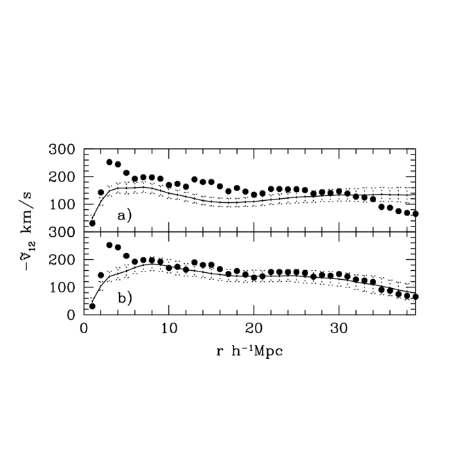
Figure 3: ${v_{{\scriptscriptstyle 12}}}(r)$ and its variance evaluated from 100 mock catalogues with errors (described in the text) and the full selection function. The solid points are the ${{\tilde{v}}_{{\scriptscriptstyle 12}}}$ of the error-free simulation seen from the same observation point, the solid line is the mean and dashed lines are the 1 $\sigma$. a) uncorrected distances; b) distances corrected for Malmquist bias

Figure 4: The effect of generalized Malmquist bias on ${\tilde{v}}_{12}(10h^{-1}\;\mbox{Mpc})$. The thick vertical line is the true value, the dashed histogram is the uncorrected estimate and the solid histogram is corrected for Malmquist bias. This is taken from 1000 realizations of log-normal errors (as described in the text). The histograms have been normalized to unity

References

- (1) da Costa, L. et al. (1996) Ap.J. 486, L5
- Davis, Nusser Willick, (1996) Davis, M., Nusser, A. Willick, J. (1996) Ap.J. 473, 22
- Davis, Pebbles, (1977) Davis, M. & Peebles, P. J. E., (1977) Ap.J.Suppl. 34, 425
- Efstathiou (1996) Efstathiou, G. (1996) in Les Houches, Session LX, Eds. Schaeffer, R. et al., (Elsevier: Amsterdam), p.133
- Fisher et al. (1994) Fisher, K.B., Davis, M., Strauss, M., Yahil A., Huchra, J. (1994) M.N.R.A.S. 267, 927
- Górski (1988) Górski, K.M. (1988) Ap.J. 332, L7
- Górski et al. (1989) Górski, K.M. et al. (1989) Ap.J. 344, 1
- Groth et al. (1989) Groth, E.J., Juszkiewicz, R., Ostriker, J.P. (1989) Ap. J. 346, 558
- (9) Juszkiewicz, R., Fisher, K., & Szapudi, I. (1998a) Ap. J. Lett., 504, L1
- (10) Juszkiewicz, R., Springel, V., & Durrer, R. (1998b) astro-ph/9812387
- Kaufmann et al. (1998) Kaufmann, G., Colberg, J.M., Diaferio, A., White, S.D.M. (1998) astro-ph/9805283.
- Landy Szalay (1992) Landy S., Szalay A. (1992) Ap.J. 391, 401
- Łokas et al. (1996) Łokas, E., Juszkiewicz, R., Bouchet, F.R., & Hivon, E. (1996) it Ap.J., 467, 1
- Peebles (1980) Peebles, P. J. E. (1980) The Large–Scale Structure of the Universe, (Princeton: Princeton University Press) (LSS)
- Peebles (1993) Peebles, P. J. E. (1993) Principles of Physical Cosmology, (Princeton: Princeton University Press) (PPC)
- Scoccimarro & Frieman (1996) Scoccimarro, R., & Frieman, J. (1996) Ap.J., 473, 620
- (17) Strauss, M., Willick, J. (1995) Phys. Rep. 261, 271
- Willick et al. (1997) Willick, J. et al. (1995) Ap.J.Supp. 109, 333