Tidal disruption rates of stars in observed galaxies

Abstract

We derive the rates of capture ${\dot{N}}$ of main sequence turn off stars by the central massive black hole in a sample of galaxies from Magorrian et al. 1998. The disruption rates are smaller than previously believed with ${\dot{N}}\sim 10^{-4}-10^{-7}$ per galaxy. A correlation between ${\dot{N}}$ and black hole mass ${M}$ is exploited to estimate the rate of tidal disruptions in the local universe. Assuming that all or most galaxies have massive black holes in their nuclei, this rate should be dominated by sub-${L_{*}}$ galaxies. The rate of tidal disruptions could be high enough to be detected in supernova (or similar) monitoring campaigns—we estimate the rate of tidal disruptions to be $0.01-0.1$ times the supernova rate. We have also estimated the rates of disruption of red giants, which may be significant (${\dot{N}}\ga 10^{-4}\hbox{y}^{-1}$ per galaxy) for ${M}\ga 10^{8}{M_{\sun}}$, but are likely to be harder to observe—only of order $10^{-4}$ times the supernova rate in the local universe. In calculating capture rates, we advise caution when applying scaling formulae by other authors, which are not applicable in the physical regime spanned by the galaxies considered here.

1 Introduction

A number of early type galaxies and spiral bulges are now thought to contain massive black holes in their nuclei (Magorrian et al. 1998). Direct evidence is also now available which supports the idea that active galaxies are powered by massive black holes (Reynolds & Fabian 1997, Fabian et al. 1998). It can be argued that many if not all galaxies could be expected to have undergone an active phase and to possess a massive black hole (Haehnelt & Rees 1993). Magorrian et al. measure black hole masses in the range ${M}=10^{6}-10^{9}{M_{\sun}}$, and report that ${M}$ is correlated with the mass $\cal M$ of the underlying hot stellar system, with ${M}/{\cal M}=x\approx 0.006$.

A main sequence star of roughly solar type can be tidally disrupted by a black hole with mass ${M}\la 2\times 10^{8}{M_{\sun}}$ (Hills 1975). Larger black holes swallow main sequence stars whole, but red giants are susceptible to tidal disruption because of their lower density. Frank & Rees (1976) (FR), Young, Shields & Wheeler (1977) considered a system composed of a black hole and an isothermal sphere of stars and derived analytic expressions for the rate of capture of stars. Cohn & Kulsrud (1978) (CK) were able to calibrate FR using a more detailed numerical calculation. Estimates of capture rates in the literature are often based on equation (66) of CK (e.g. Cannizzo, Lee & Goodman 1990, Kormendy & Richstone 1995). We argue that such estimates are often wrong because the physical conditions in galactic nuclei are different from those anticipated by CK (who were in any case more concerned with globular clusters).

The next section summarises briefly what is known about the observational signatures of tidal disruption. Section 3 establishes notation by reviewing the analytic theory of FR and sets out our method for calculating capture rates in the Nuker galaxies. We calibrate our calculation against the result of CK. In Section 4 we describe the data and list the quantities we derive from them, including capture rates. We discuss our results in Section 5.

2 Observability

The observable consequences of such an event have been discussed by Rees (1988), Evans & Kochanek (1989), Canizzo, Lee & Goodman (1990) and Ulmer (1997). The general expectation for the disruption of a main sequence star is a flare with bolometric luminosity near the Eddington limit. In comparison, the luminosity from the central $r<1\,$arcsec of all the Nuker galaxies is small compared to the Eddington luminosity of the black hole ($\la 10^{-4}L_{\rm Edd}$, Table 1). The bolometric luminosity should be close to the Eddington limit because of the predicted mass accretion rates are above the Eddington accretion rate for black holes with mass up to about $3\times 10^{7}~{}{M_{\sun}}$. Above that the predicted mass accretion rate divided by the Eddington mass accretion rate falls as $M^{3/2}$ (Ulmer 1997). There is much uncertainty as to how optically bright a tidal disruption event will be, in optical, but the minimum luminosity expected for typical disruptions of main sequence stars is $10^{-3}{-}10^{-2}L_{\rm Edd}$ for the U and V bands (Ulmer 1997). Typical durations of the brightest phase will be $0.1{-}2$ years depending on the black hole mass. Main sequence tidal disruption events should therefore be relatively easy to detect as a byproduct of supernova searches (Section 4.1) or other searches which observe the same galaxies many times over (e.g. Southern strip of the SDSS).

Red giant disruption events are generally much longer lasting, and therefore fainter, than main sequence events. Red giants typically are disrupted by growing onto the loss cone (Section 3.2), so at disruption, they have pericenter equal to the tidal disruption radius. Consequently, an average red giant (with $R\sim 100{R_{\sun}}$) disruption has a approximate duration of $100M_{6}^{1/2}$ years and a produces a peak mass accretion rate no larger than $\sim 10^{-3}~{}M_{6}^{-1/2}{M_{\sun}}$ yr^-1 (see Ulmer 1997, eqs 3,5). The Eddington accretion rate, which would supply enough mass to provide the Eddington luminosity, is $3\times 10^{-2}M_{6}\epsilon^{-1}_{.1}$, where $0.1\times\epsilon_{.1}$ is the efficiency of rest mass to light conversion in the accretion process. This means that red giant disruption could keep a small, $10^{6}~{}{M_{\sun}}$ black hole illuminated at (1/30th) its Eddington rate for up to a thousand years.

Just how bright a red giant disruption would appear in optical bands is difficult to determine, but a simple estimate is as follows. If most of the energy is released from within a few Schwarzschild radii for both the main sequence and red giant disruptions, and the bolometric luminosity of the red giant disruptions is 1/30 that of the main sequence disruptions for a $10^{6}~{}{M_{\sun}}$ black hole, then

$${1\over 30}\sim{L_{\rm{RG}}\over L_{\rm MS}}\sim{T_{\rm eff,{\rm{RG}}}^{4}\over T_{\rm eff,MS}^{4}}.$$ (1)

Therefore, the ratio of temperatures is $(1/30)^{1/4}\sim 0.4$. Because the optical bands lie in the Rayleigh-Jeans tail of the spectrum where the luminosity scales linearly with $T$, we would at first guess expect that red giant disruptions would be nearly (i.e. $\sim 0.4$ times) as bright as main sequence events. Around more massive black holes with $M\sim 10^{8}{M_{\sun}}$, red giants may be significantly less luminous if the accretion becomes advection dominated as appears to be the case for many extra-galactic black holes with accretion rates far below the Eddington accretion rate (e.g. NGC 4258 (Lasota et al. 1996), M87 (Reynolds et al. 1996)). Around very massive black holes with $M\sim 10^{10}M_{\odot}$, the timescale for return of the disruption material to the black hole becomes comparable with the interval between successive tidal disruptions (see Figure 4). Red giant disruptions would then provide a small, nearly constant flow of material onto the black hole of $\sim 10^{-3}M_{\odot}{\rm yr}^{-1}$ corresponding to a luminosity of $\sim 10^{-5}\epsilon_{.1}L_{\rm Edd}$

3 Theory of capture rates

Consider a spherical cluster of stars of mass $m_{*}$ with density $\rho(r)$, and isotropic velocity dispersion $\sigma(r)$. Typically $\rho(r)$ is in the form of two power laws, separated by a break radius $r_{\rm b}$. The velocity dispersion is then given by Jeans’ equations:

$${{\rm d}\rho\sigma^{2}\over{\rm d}r}+{G\rho{\cal M}(r)\over r^{2}}=0$$ (2)

where ${\cal M}(r)$ is the mass enclosed within radius $r$, including the black hole, and $G$ is Newton’s constant. The black hole exerts an influence on the stars inside a sphere of influence with radius $r_{\rm a}$ given by

$${G{M}\over r}-\sigma(r)^{2}=0,$$ (3)

where ${M}$ is the black hole mass. Within the sphere of influence ($r<r_{\rm a}$)

$$\sigma^{2}\approx{G{M}\over(1+p)r},$$ (4)

where the logarithmic slope of the density is $-p$ (i.e. $\rho\sim r^{-p}$, with $p$ possibly dependent on radius). An important derived quantity is the two-body relaxation timescale, given by

$$t_{\rm r}={\sigma^{3}\over\Lambda G^{2}\rho m_{*}},$$ (5)

where $m_{*}$ is the typical stellar mass and $\Lambda$ includes dimensionless factors of order unity as well as the Coulomb logarithm. We use the numerical value of $t_{\rm r}$ given by Binney & Tremaine 1987, equation (8-71). Since $t_{\rm r}$ is not very sensitive to $\Lambda$ we do not attempt to include the dependence of $\Lambda$ on $r$. Instead we take

$$t_{\rm r}=$$ (6)

$$\kern-10.00002pt{1.8\times 10^{12}\hbox{y}\over\ln(0.4N)}\left(\sigma\over 100\hbox{km\,s${}^{-1}$}\right)^{3}\left({M_{\sun}}\over m_{*}\right)\left(10^{4}{M_{\sun}}\hbox{pc}^{-3}\over\rho\right),$$

where $N$ is the number of stars within the characteristic radius $r_{\rm b}$.

3.1 The loss cone

Suppose that stars are removed from the system if they come within a distance $q$ of the centre of the cluster. If there is a massive black hole at the centre, $q$ will be the larger of the tidal radius $r_{\rm T}\approx R_{\star}({M}/M_{\star})^{1/3}$ (Hill 1975) or the Schwarzschild radius of the black hole. For stars at the main sequence turn off, $q=r_{\rm T}$ when ${M}\la 2\times 10^{8}{M_{\sun}}$. A star at radius $r$ will be removed if its angular momentum is small enough. Such stars are said to populate a ‘loss-cone’ (Lightman & Shapiro 1977, Young, Shields & Wheeler 1977, FR), the angular size of which is given at radius $r$ by

$$\theta_{\rm lc}^{2}={q\over r^{2}}{G{M}\over\sigma^{2}}$$ (7)

(provided $\sigma^{2}\ll{M}/q$). Even at the edge of the sphere of influence, the loss cone is quite small with $\theta_{\rm lc}\sim 10^{-7}-10^{-5}$.

The loss process is usually divided into two regimes according to the angle $\theta_{\rm d}$ through which a star is scattered in a dynamical time

$$t_{\rm d}=r/\sigma.$$ (8)

In the ‘diffusive’ regime $\theta_{\rm d}<{\theta_{\rm lc}}$, and on timescales much longer than $t_{\rm d}$ the loss cone is empty, because a star which finds itself in the loss cone is removed within a dynamical time. In this case, the capture rate is limited by diffusion into the loss cone, and is given, per star, by

$${{\rm d}{\dot{N}_{<}}\over{\rm d}N}={1\over\ln(2/{\theta_{\rm lc}})t_{\rm r}}$$ (9)

(Lightman & Shapiro 1977), where $N(r)$ is the number of stars contained within a radius $r$.

In the other regime, $\theta_{\rm d}>{\theta_{\rm lc}}$, the loss cone is always full. Since we assume isotropic velocity dispersions, the fraction of stars in the loss cone at any time is just ${\theta_{\rm lc}}^{2}$. Thus in this case the capture rate per star is

$${{\rm d}{\dot{N}_{>}}\over{\rm d}N}={{\theta_{\rm lc}}^{2}\over t_{\rm d}}.$$ (10)

The rates (9) and (10) are equal at a radius $r={r_{\rm crit}}$, where

$${G\rho r^{3}\over\sigma^{2}}=q{{M}\over m_{*}}\Lambda_{\rm lc}$$ (11)

where we have written $\Lambda_{\rm lc}=\ln(2/{\theta_{\rm lc}})/\Lambda$. The radial dependence of $\Lambda_{\rm lc}$ is weak, so we set it to a constant equal to its value at $r_{\rm b}$.

The first step in calculating the capture rate is to solve equation (11) to find ${r_{\rm crit}}$. Then we can find the total loss rate, ${\dot{N}}$, by integrating equations (9) and (10) over the cluster:

$${\dot{N}}={\dot{N}_{<}}\;+\;{\dot{N}_{>}},$$ (12)

with

$${\dot{N}_{<}}=4\pi\int\limits_{0}^{r_{\rm crit}}\;{\Lambda_{\rm lc}G^{2}\rho^{2}r^{3}\over\sigma^{3}}\;{{\rm d}r\over r}$$ (13)

$${\dot{N}_{>}}=4\pi\int\limits_{r_{\rm crit}}^{\infty}\,{G{M}q\rho\over m_{*}\sigma}\;{{\rm d}r\over r}.$$ (14)

Before moving on, let us examine the various contributions to ${\dot{N}}$ in some more detail. Let us define $f(r)$ to be the $r$-dependence of the integrand in ${\dot{N}_{<}}$, so

$$f(r)={G^{2}\rho^{2}r^{3}\over\sigma^{3}}$$ (15)

Now at small $r$, $\sigma\sim r^{-1/2}$, so $f(r)\to 0$ as $r\to 0$ provided $p<9/4$ (which is true in all the galaxies we consider). The lower limit in the first integral in principle should be finite, but for $p<9/4$ we may set it to zero. At large radius,

$$\sigma^{2}\sim r^{2-p} p<3$$ , (16)

$$\sigma^{2}\sim r^{-1/2} p>3$$ , (17)

so $f(r)\to 0$ as $r\to\infty$ provided $p>0$. Thus generally $f(r)$ will reach a maximum at some radius $r_{\rm max}$. Quite generally we expect that $r_{\rm max}$ will be approximately equal to $r_{\rm a}$ (for $r_{\rm a}<r_{\rm b}$ or $0<p<9/4$ at large $r$) or $r_{\rm b}$ (otherwise). We can identify two distinct regimes according to whether ${r_{\rm crit}}\grole r_{\rm max}$ .

1. If ${r_{\rm crit}}\gg r_{\rm max}$ then ${\dot{N}_{>}}$ will be insignificant compared to ${\dot{N}_{<}}$.

2. If ${r_{\rm crit}}\la r_{\rm max}$ then ${\dot{N}_{>}}$ will be at most comparable with ${\dot{N}_{<}}$.

In case 1

$${\dot{N}}\approx{\dot{N}}_{\rm max}={N(r_{\rm max})\over t_{\rm r}(r_{\rm max})}$$ (18)

and in case 2

$${\dot{N}}\approx{\dot{N}}_{\rm crit}={N({r_{\rm crit}})\over t_{\rm r}({r_{\rm crit}})}.$$ (19)

Equations (18) and (19) constitute a poor man’s recipe for calculating capture rates, and within a factor of order unity are interchangeable with the full integral version in equation (12).

3.2 Red giant capture

For black hole masses $\ga 2\times 10^{8}{M_{\sun}}$, the Schwarzschild radius exceeds the tidal disruption radius for main sequence stars. Red giants, as a result of their low densities, have much much larger tidal radii, and can therefore be disrupted. Red giants may enter the loss cone in the same manner as main sequence stars: they diffuse towards an empty loss cone for orbits below a critical radius, and above that radius, they scatter onto a full loss cone. There is an additional contribution to the red giant capture rate. Red giants also grow onto the loss cone as they expand. The loss cone for red giants is larger than for main sequence stars ($q$ is larger because they are less dense), so even when the main sequence loss cone is empty, red giants are being born inside their own loss cone. While the total fraction of stars which are red giants at any given time may be very small, the number of red giants susceptible to capture may be significant. We discuss each of these capture channels below. In addition, throughout this discussion we use the term red giant loosely to describe stars on both the RGB and AGB.

3.2.1 Radius-time relationship

In order to calculate the capture rates, it is necessary to understand how red giants evolve in radius as a function of time because the loss cone, $\theta_{\rm lc}\propto R_{\star}$ (7). A good estimate of the radius evolution can be easily determined as the radius and luminosity of a red giant are largely independent of the stellar mass, and depend only on the core mass. Functional forms for $L(m_{\rm c})$ and $R(m_{\rm c})$ are given in Joss, Rappaport & Lewis (1987) , where $m_{\rm c}$ is the core mass, which are good approximations for both the red giant and ascending red giant branches. Because the dominant energy source in red giants is the $p{-}p$ chain with $\sim 0.7$% efficiency and the core mass is increased as hydrogen burns to helium, we may write

$$L(m_{\rm c}) \approx 0.007{M_{\sun}}c^{2}\;{\partial\mu\over\partial t}$$ (20)

$$\approx {10^{5.3}\mu^{6}\over 1+10^{0.4}\mu^{4}+10^{0.5}\mu^{5}}{L_{\sun}},$$ (21)

where $\mu=m_{\rm c}/{M_{\sun}}$, and the right hand side comes from Joss, Rappaport & Lewis (1987). Solving this equation for core mass as a function of time, gives the luminosity-time dependence. A similar expression to equation (21) yields the radius-time dependence.

Applying this model between an initial core mass of 0.17 ${M_{\sun}}$ and a final core mass of 0.8 ${M_{\sun}}$ we find an initial radius of 3.09 ${R_{\sun}}$ and a maximum radius, $R_{\rm max}$, of 679 ${R_{\sun}}$ after $7\times 10^{8}$ years. This maximum radius is in fact larger than the radius predicted by stellar evolution codes, because mass loss significantly alters the evolution, especially when in the star reaches the thermally pulsing AGB phase (TPAGB). We therefore limit the red giant evolution at $200{R_{\sun}}$ which corresponds to the onset of the TPAGB (e.g. Bressan et al. 1992).

For our level of approximation of the red giant capture rates, a simple analytical expression for the radius-time dependence is sufficient. A course approximation (figure 1) is:

$${t\over 7\times 10^{8}{\rm years}}\approx 0.38\ln\left({R\over{R_{\sun}}}-3\right)+.37.$$ (22)

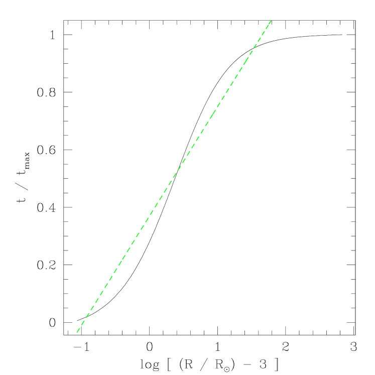
Figure 1: Time as a function red giant radius (solid line). The dashed line shows an approximation adopted in eq. 22.

3.2.2 Red giant birth rate and number density

In order to calculate the red giant capture rates, we must determine their birth rate and their number density.

The main sequence lifetime of a star of mass $m$ is given approximately by

$$t_{\rm ms}\sim 10^{10}\left(m\over{M_{\sun}}\right)^{-2.5}\hbox{y}$$ (23)

and the total number of stars, assuming a Salpeter mass function, is

$${{\rm d}N\over{\rm d}m}\approx 1.6\left(m\over{M_{\sun}}\right)^{-1.35},$$ (24)

where the total mass has been normalised to unity in the range $(0.3,0.8){M_{\sun}}$. Therefore the birth rate of red giants (per star) is

$${{\rm d}\dot{N}_{\rm new}\over{\rm d}N} = {{\rm d}N\over{\rm d}m}\;{\left|{{\rm d}m\over{\rm d}t}\right|}$$ (25)

$$\approx 0.65\times 10^{-10}\left(m\over{M_{\sun}}\right)^{2.15}\hbox{y}^{-1},$$

where $m$ is now the main sequence turn off mass (the mass of stars which are currently being transformed into red giants). The total red giant lifetime $t_{\rm{RG}}\sim 7\times 10^{8}\hbox{y}$, so the fraction of stars that are red giants (with radii between $\sim 3$ and $200{R_{\sun}}$) is

$$f_{\rm{RG}}={{\rm d}\dot{N}_{\rm new}\over{\rm d}N}\,t_{\rm{RG}}\approx 0.05.$$ (26)

We therefore expect that the red giant capture rate will be lower than the main sequence rate by no more than a factor of 20. Another important quantity is the time averaged radius, ${<}R{>}\sim 12{R_{\sun}}$. The evolution above $100{R_{\sun}}$ makes only a small ($<$10%) contribution to the time averaged radius.

3.2.3 Maximum radius limits

The red giant capture rates depend on the maximum radius reached by the red giant. We consider how this radius may be truncated by stellar collisions, and how this radius can effectively be truncated when the red giant evolution time becomes shorter than the dynamical time.

First, consider the frequency of collisions between a red giant and a main sequence star:

$${t_{\rm coll}\over t_{\rm r}}\approx{3.7\ln{0.4N}\theta^{2}\over 1+2\theta},$$ (27)

where $\theta$ is the Safronov number, $Gm_{*}/2\sigma^{2}R$ (see Binney & Tremaine 1987, equation 126). for $\sigma\sim 100\hbox{km\,s${}^{-1}$}$, $\theta$ varies between about 5 and 0.01 as a red giant evolves. The collisions are important if a red giant typically collides during its lifetime:

$$\int_{R_{\rm min}}^{R_{\rm max}}{{\rm d}t\over t_{\rm coll}R}\approx 1,$$ (28)

where $R_{\rm min}\approx 3{R_{\sun}}$. Using the relations from section 3.2.1 and setting $\ln(0.4N)\sim 20$, we find that collisions are important when

$$t_{\rm r}\la 1.1\times 10^{7}\left({250\hbox{km\,s${}^{-1}$}\over\sigma}\right)^{3}{\rm years}.$$ (29)

For the systems we consider here, the shortest relaxation times (at $r_{\rm a}$) are many tens of times too large for collisions to be important.

Second, at large system radii, the most extended red giants may evolve on a time faster than the dynamical time, so that extended red giants have a reduced chance of encountering the black hole. Using the red giant evolution model from Section 3.2.1, we calculate the characteristic evolution time, $R/\dot{R}$ as a function of radius (Figure 2). We find that over the radii range $3{-}200{R_{\sun}}$, the relationship is well approximated by

$$t_{R}\equiv R/\dot{R}\sim 6.5\times 10^{6}\left({R\over 200{R_{\sun}}}\right)^{-1.12}.$$ (30)

The maximum radius for a red giant is therefore the smaller of $200{R_{\sun}}$ and the radius at which $t_{R}=t_{\rm d}$. In practice for the Nuker galaxies in the regions of interest $t_{R}$ is always much greater than $t_{\rm d}$, and we take $R_{\rm max}=200{R_{\sun}}$.

Figure 2: Characteristic evolution time, $R/\dot{R}$ as a function radius for red giants (solid line). The dashed line shows an simple fit to the model.

3.2.4 Capture analogous to main sequence capture

Main sequence capture occurs by diffusion onto an empty loss cone at radii below the critical radius, and by scattering onto a full loss cone above the critical radius (equations 9, 10). In general, the larger the radius of the star, the larger the critical radius, and at large radii, the critical radius scales as the stellar radius (equations 11, 16). For red giants we must define three regions because the red giant radius and therefore the critical radius are functions of time. Below a radius ${r_{\rm crit,1}}$ determined by solving equation (11) with $q=3q_{\rm ms}$, the loss cone is depleted on a dynamical time for all red giants, so the diffusion rate is appropriate. Beyond the second radius ${r_{\rm crit,2}}$ determined by solving equation (11) with $q=200q_{\rm ms}$, the loss cone is full, so the full loss cone rate is appropriate. Between these two radii, the full rate is appropriate until the star reaches a size at which it can scatter entirely into or out of the loss cone in one dynamical time, i.e. the stellar radius $R_{t}$ for which equation (11) is satisfied. The rate of captures of red giants from these three contributions can therefore be written:

$${{\rm d}{\dot{N}}_{\rm{RG}}\over{\rm d}N}=$$ (31)

$$\kern-45.0pt{{\rm d}\dot{N}_{\rm new}\over{\rm d}N}\left[\int_{R_{\rm min}}^{R_{t}}{R\over{R_{\sun}}}{{\rm d}t\,{\theta_{\rm lc}}^{2}\over t_{\rm d}}+\int_{R_{t}}^{R_{\rm max}}{{\rm d}t\over\ln(2/{\theta_{\rm lc}})t_{\rm r}}\right].$$

The limits in the integrals are understood to mean the time at which $R$ is equal to the value specified. The critical red-giant radius $R_{t}$ is equal to $R_{\rm min}$ for $r<{r_{\rm crit,1}}$ and to $R_{\rm max}$ for $r>{r_{\rm crit,2}}$.

3.2.5 Captures from growth onto the loss cone

There will be some maximum radius for red giants $R_{\rm max}$, fixed either by stellar evolution (at $\sim 200{R_{\sun}}$), or by other means e.g, the rate at which their envelopes are stripped by collisions with other stars. As we discuss below, the appropriate maximum radius is almost always set by stellar evolution. This maximum radius defines a loss cone with angular size

$$\theta_{\rm{RG}}^{2}={\theta_{\rm lc}}^{2}{R_{\rm max}\over{R_{\sun}}},$$ (32)

where (as before) ${\theta_{\rm lc}}$ is the angular size of the main sequence loss cone. Assuming that all stars which become red giants inside this loss cone will be captured, the rate of red giant captures from a given radius (per star) is

$${{\rm d}{\dot{N}}_{\rm{RG}}\over{\rm d}N}={\theta_{\rm{RG}}^{2}{{\rm d}\dot{N}_{\rm new}\over{\rm d}N}}\approx{460{\theta_{\rm lc}}^{2}\over t_{0}}\approx{4.6\times 10^{-8}{\theta_{\rm lc}}^{2}}\hbox{y}^{-1},$$ (33)

where $t_{0}$ is the age of the galaxy, and we have chosen $R_{\rm max}=200{R_{\sun}}$.

3.2.6 Total capture rate

The rate of red giant capture per star is the sum of equations (31) and (33):

$${{\rm d}{\dot{N}}_{\rm{RG}}\over{\rm d}N} = {\textstyle{\rm d}\dot{N}_{\rm new}\over\textstyle{\rm d}N}\left[\int_{R_{\rm min}}^{R_{t}}{R\over{R_{\sun}}}{{\rm d}t\,{\theta_{\rm lc}}^{2}\over t_{\rm d}}+\right.$$ (34)

$$\;\;\left.\int_{R_{t}}^{R_{\rm max}}{{\rm d}t\over\ln(2/{\theta_{\rm lc}})t_{\rm r}}\,+\,{R_{\rm max}\over{R_{\sun}}}{\theta_{\rm lc}}^{2}\right],$$

which must be integrated over the system to obtain the total capture rate

$${\dot{N}}_{\rm{RG}}=4\pi\int_{0}^{\infty}{{\rm d}{\dot{N}}_{\rm{RG}}\over{\rm d}N}\rho r^{2}{\rm d}r.$$ (35)

For the Nuker galaxies, since ${r_{\rm crit}}$ is generally large for main-sequence stars it is larger still for red giants, and $R_{t}=R_{\rm min}$. We also find that growth onto the loss cone (equation 33) dominates the red giant capture rate.

3.3 Calibration

FR considered a system in which the stars inside the sphere of influence have relaxed to the ‘zero-flow’ distribution of Bahcall & Wolf (1976) with $p=7/4$, and outside $r_{\rm a}$ the stars are approximately isothermal with a homogeneous core of radius $r_{0}$ and density $\rho_{0}$. One case they concentrated on was that in which ${r_{\rm crit}}<r_{\rm a}<r_{0}$. CK also calculated the capture rate (as well as the full anisotropic distribution function) in a system with ${r_{\rm crit}}<r_{\rm a}$ and a relaxed cusp with $p\approx 1.8$. They give a scaling relation (their equation 66) for ${\dot{N}}$ in these circumstances which is substantially the same as FR equation (16a), except for the normalisation. We use this normalisation to calibrate our model capture rates.

Table 1: Observational data and summary of results. Column (2) taken from Byun et al. 1996; Columns (3-4) from Magorrian et al. 1998. Column (1), name of galaxy; (2), $r_{\rm b}$ in pc; (3), Nuker law indices $(\alpha,\beta,\gamma)$; (4) $\log_{10}{M}$ black hole mass; (5) $r_{\rm a}/r_{\rm b}$; (6) $r_{\rm a}$ in arcsec; (7) main-sequence capture time (${\dot{N}}$/y); (8) red giant capture time (${\dot{N}}_{\rm{RG}}$/y); (9) projected stellar luminosity in central arcsec $\ell(1)=L(r<1")/L_{\rm Edd}$.

NGC	$r_{\rm b}$	$(\alpha,\beta,\gamma)$	$\log{M}$	$r_{\rm a}\over r_{\rm b}$	$r_{\rm a}(")$	$-\log{\dot{N}}$	$-\log{\dot{N}}_{\rm{RG}}$	$-\log\ell(1)$
1399	$269.15$	$(1.50,1.68,0.07)$	$9.72$	$0.38$	$1.19$	$6.13$	$4.23$	$4.92$
1600	$1258.93$	$(1.98,1.50,0.08)$	$10.06$	$0.09$	$0.48$	$6.60$	$3.92$	$5.02$
2832	$398.11$	$(1.84,1.40,0.02)$	$10.06$	$0.51$	$0.46$	$6.41$	$4.09$	$4.36$
3115	$117.49$	$(1.47,1.43,0.78)$	$8.55$	$0.07$	$0.19$	$4.80$	$4.46$	$3.47$
3377	$4.37$	$(1.92,1.33,0.29)$	$7.79$	$0.97$	$0.09$	$4.80$	$5.10$	$2.99$
3379	$83.18$	$(1.59,1.43,0.18)$	$8.60$	$0.22$	$0.38$	$5.76$	$5.00$	$4.02$
608	$27.54$	$(1.05,1.33,0.00)$	$8.39$	$0.54$	$0.15$	$5.54$	$5.10$	$3.51$
168	$446.68$	$(0.95,1.50,0.14)$	$9.08$	$0.19$	$0.48$	$6.47$	$5.00$	$4.11$
4467	$239.88$	$(7.52,2.13,0.98)$	$7.44$	$0.04$	$0.13$	$5.36$	$5.76$	$3.13$
4472	$177.83$	$(2.08,1.17,0.04)$	$9.42$	$0.17$	$0.41$	$6.05$	$4.20$	$4.93$
4486	$562.34$	$(2.82,1.39,0.25)$	$9.55$	$0.14$	$1.06$	$6.32$	$4.39$	$5.21$
4486	$13.49$	$(2.78,1.33,0.14)$	$8.96$	$9.95$	$1.81$	$5.90$	$5.02$	$4.38$
4552	$47.86$	$(1.48,1.30,0.00)$	$8.67$	$0.24$	$0.15$	$5.57$	$4.75$	$3.80$
4564	$38.90$	$(0.25,1.90,0.05)$	$8.40$	$0.37$	$0.20$	$5.24$	$4.90$	$3.34$
4621	$218.78$	$(0.19,1.71,0.50)$	$8.45$	$0.03$	$0.10$	$4.74$	$4.52$	$3.09$
4636	$239.88$	$(1.64,1.33,0.13)$	$8.36$	$0.07$	$0.24$	$6.24$	$5.35$	$4.07$
4649	$263.03$	$(2.00,1.30,0.15)$	$9.59$	$0.29$	$1.04$	$6.19$	$4.32$	$5.11$
4874	$1202.26$	$(2.33,1.37,0.13)$	$10.32$	$0.39$	$1.04$	$6.93$	$4.13$	$5.12$
4889	$758.58$	$(2.61,1.35,0.05)$	$10.43$	$0.64$	$1.07$	$6.72$	$3.96$	$4.89$
6166	$1202.26$	$(3.32,0.99,0.08)$	$10.45$	$0.68$	$1.50$	$7.16$	$4.18$	$5.42$
7332	$75.86$	$(4.25,1.34,0.90)$	$6.84$	$0.01$	$0.01$	$4.10$	$4.81$	$1.31$
7768	$199.53$	$(1.92,1.21,0.00)$	$9.96$	$1.25$	$0.50$	$6.34$	$4.17$	$4.25$
221	$1.47$	$(2.00,1.28,0.53)$	$6.36$	$0.50$	$0.19$	$4.53$	$5.27$	$3.05$
224	$288.40$	$(1.12,1.52,0.33)$	$7.79$	$0.04$	$2.80$	$5.95$	$5.76$	$5.41$
MW	$0.38$	$(1.80,0.80,0.00)$	$6.42$	$1.23$	$11.38$	$4.32$	$5.07$	$6.80$

$\mu_{\rm V}\,(\hbox{mag/arcsec${}^{2}$})$

$r\,(\hbox{arcsec})$

Figure 3: Deconvolved V-band surface density of M31 (triangles) with Nuker law fits to the inner ($r<1.75"$) and outer ($r>3.6"$) profiles (dotted lines).

4 The Nuker galaxies

To calculate a capture rate, we need to know the density profile $\rho(r)$ and the black hole mass ${M}$. Given the observed surface brightness $I(r)$, we can derive $\rho(r)$ by an Abel inversion, assuming a constant mass-to-light ratio $\Upsilon$. We do not assume anything about the density profile in regions which are not resolved by the observations, merely extrapolating the profiles inwards. This will not affect the capture rates provided min$[{r_{\rm crit}},r_{\rm max}]$ is not much smaller than the resolution limit of the observations, which turns out to be the case. Most of the data we use are quoted as a Nuker law fit to $I(r)$ (Byun et al. 1996). Thus $I(r)$ is in the form of two power laws, separated by a break radius $r_{\rm b}$, and $\rho(r)$ has a similar form, with a break radius close to $r_{\rm b}$. The data we have used are reproduced in Table 1, which also lists some interesting derived quantities. M32 is listed as NGC 221, M31 is NGC 224, and the Milky Way is ‘MW’. The Milky Way data is from the model by Genzel et al. 1996. The Nuker parameters for M32 are taken from Lauer et al. (1992). For M31 we fit the photometry ourselves using data from Lauer et al. (1993) ($r<10"$) and Kent (1987) ($r>10"$) and matching at $r=10"$. The resulting surface density profile is shown in Figure 3, which also shows the Nuker law fits listed in Table 1. We fit the nuclear component ($r<1.75"$) separately, and name it NGC 224N in Table 1. This component is not self gravitating and is probably rotationally supported (Lauer et al. 1993, Tremaine 1995), and the capture rate is therefore almost certainly much less than in our isotropic model. We calculate the latter in order to satisfy ouselves that the capture rate is not dominated by the nuclear component, which is confirmed by the results. The scale of the flattened component in M31 is much smaller than the physical scale which dominates stellar capture rates. Similarly, in the other galaxies the capture rate is dominated by a physical radius which is well resolved, so unresolved substructure should not affect our results.

Throughout this section we assume where necessary that the mass of the black hole is proportional to the mass of the galaxy (or spheroid) with constant of proportionality $\approx.006$ (Magorrian et al. 1998), and the mass to light ratio obeys the fundamental plane relation $\Upsilon\propto L^{0.2}$. Thus the black hole mass is

$${M}\approx 6\times 10^{8}\left(L\over L_{*}\right)^{1.2}.$$ (36)

${\dot{N}}(\hbox{y}^{-1})$

${M}({M_{\sun}})$

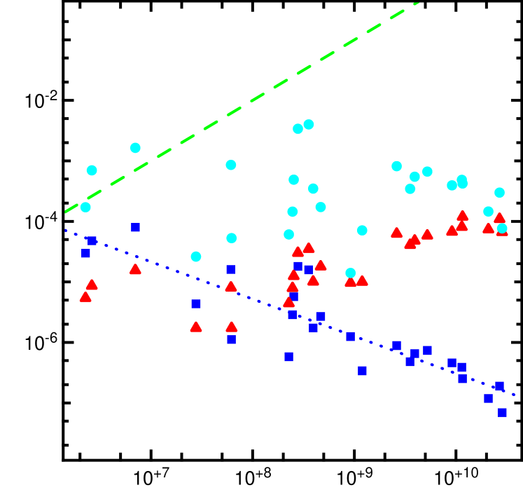
Figure 4: The capture rates ${\dot{N}}(\hbox{y}^{-1})$ for main sequence stars (squares) and red giants (triangles) as a function of black hole mass. The circles are the main sequence capture rates in the case where loss cones are all full. The dotted line is the best fit to the main sequence rates (with loss cone), and has slope $-0.61$. The dashed line is the upper limit set by ${\dot{N}}m_{*}={M}/t_{0}$ with $t_{0}=10^{10}\hbox{y}$.

4.1 Capture rates

Figure 4 shows the capture rates as a function of the black hole mass. In our models all the Nuker galaxies have ${r_{\rm crit}}\gg r_{\rm b}$ and all but two have $r_{\rm b}\ga r_{\rm a}$, and hence $r_{\rm max}\approx r_{\rm a}$. This accounts for why both the main sequence rate and the red giant rate are correlated with ${M}$. In the red giant case, the capture rate is proportional to the mass within $r_{\rm a}$ which is of order the black hole mass. In the main sequence case the fuelling rate is proportional to this mass divided by $t_{\rm r}(r_{\rm a})$. The fundamental plane leads to a correlation between $t_{\rm r}(r_{\rm a})$ and $M$, and hence to the correlation in Figure 4. We can also calculate ${\dot{N}}_{\rm max}$ equation (18), and the result is well correlated with the value of ${\dot{N}}$ given in Table 1 (over a range in ${\dot{N}}$ of 3 orders of magnitude ${\dot{N}}_{\rm max}$ is within a factor of two or so of ${\dot{N}}$). We can also use equation (18) to estimate what the effect on ${\dot{N}}$ would be of errors in the determination of the black hole mass. The result for main sequence stars and empty loss cones is that errors in ${M}$ tend to move ${\dot{N}}$ roughly along the ${\dot{N}}{-}{M}$ relation in Figure 4 (dotted line).

4.1.1 Comparison with supernova rate

Main sequence capture is faster for smaller black holes, and this leads us to expect that the total rate of capture in the local universe will be dominated by the galaxies with smallest black holes. To see this more clearly, let us compare the rate of star capture with the supernova rate in the local universe. We assume a galaxy population with luminosity function of the form

$${{\rm d}N\over{\rm d}L}\propto{1\over L}\left(L\over{L_{*}}\right)^{\alpha}\exp\left(-L\over{L_{*}}\right),$$ (37)

(Schechter 1976) where empirically $\alpha$ is typically small and negative. We adopt $\alpha=-0.07$, and ${L_{*}}=1.8\times 10^{10}{L_{\sun}}$ (Estafthiou et al. 1988). The supernova rate in a galaxy is roughly proportional to its luminosity $L$. In the local universe it is approximately

$$\dot{N}_{\rm SN}\approx 10^{-2}{L\over{L_{*}}}\hbox{y}^{-1},$$ (38)

and the rate of capture of stars from Figure 4 and equation (36) is

$${\dot{N}}\approx 2\times 10^{-6}\left(L\over{L_{*}}\right)^{-s}\hbox{y}^{-1}.$$ (39)

Together with the fundamental plane relation between $\Upsilon$ and $L$, Figure 4 gives $s\approx 0.61\times 1.2=0.73$. The ratio of the star capture rate to the supernova rate is

$$f_{*}\approx{\displaystyle\int{\dot{N}}(L){{\rm d}N\over{\rm d}L}{\rm d}L\over\displaystyle\int\dot{N}_{\rm SN}(L){{\rm d}N\over{\rm d}L}{\rm d}L},$$ (40)

whence

$$f_{*}\approx 2\times 10^{-4}\;{\alpha+1\over s-\alpha}\left({L_{*}}\over L_{\rm min}\right)^{s-\alpha}$$ (41)

where $L_{\rm min}$ is the smallest luminosity for which we think the majority of galaxies have a massive black hole.

The value of $L_{\rm min}$ is not determined by observations, since most of the observations are limited to larger systems. M32 ($L=3.7\times 10^{8}{L_{\sun}}$) is the smallest galaxy in the Nuker sample with a confirmed black hole, but it is also an unusually dense system at this luminosity. Dwarf galaxies in general are usually thought not to contain black holes. For the sake of argument consider $L_{\rm min}=10^{8}{L_{\sun}}$, from which equation 41 predicts that for every supernova there would be $\sim 0.01$ tidal disruptions. If we take $L_{\rm min}=10^{7}{L_{\sun}}$ that number goes up to $\sim 0.1$. With searches now detecting many tens of supernovae, these numbers suggest that the same surveys or similar ones at shorter wavelength should uncover tidal disruptions at an interesting rate.

The rate of red giant captures ${\dot{N}}_{\rm{RG}}$ is approximately proportional to $M$. From Figure 4 we can read off the constant of proportionality and use equation (36) to write

$${\dot{N}}_{\rm{RG}}\approx 10^{-5}\left(L\over{L_{*}}\right)^{t}\hbox{y}^{-1}.$$ (42)

with $t\approx 1.2$. However, some of the corresponding tidal disruption events will have a very long timescale, and hence may not be detected as flares. Suppose we can only observe flares in cases where the return time for tidal debris $t_{\rm min}$ is less than 10y (see Ulmer 1997 for details). Then the maximum radius of a red giant whose disruption would be observable is

$$R_{\rm vis}\approx 100{R_{\sun}}\left(t_{\rm min}\over 10\hbox{y}\right)^{2/3}\left({M}\over 10^{6}{M_{\sun}}\right)^{-1/3}\;.$$ (43)

Since red giant disruption is dominated by stars growing onto the loss cone , the rate of disruptions up to $R_{\rm vis}$ is proportional to $R_{\rm vis}$, and thus

$${\dot{N}}_{\rm vis}\approx 6\times 10^{-7}\left(t_{\rm min}\over 10\hbox{y}\right)^{2/3}\left(L\over{L_{*}}\right)^{2t/3}\hbox{y}^{-1}.$$ (44)

Integrating over the luminosity function we obtain

$$f_{\rm*vis}\approx 6\times 10^{-5}\left(t_{\rm min}\over 10\hbox{y}\right)^{2/3}\;{\alpha+1\over 2t+3\alpha},$$ (45)

where $f_{\rm*vis}$ is the ratio of the rate of visible red giant disruptions to the supernova rate, so the red giant capture rate is probably much less than the main sequence capture rate in the local Universe. Note however that it is not possible to rule out intermittent behaviour in the accretion of tidal debris (e.g. Lee, Kang, & Ryu 1996) and so equation (45) represents a lower limit to the rate of detectable red giant disruptions.

4.1.2 Upper limits to capture rate

An upper limit to the capture rate is often given as the full-loss cone rate in the region $r<{r_{\rm crit}}$. If non-axisymmetric processes can keep the loss-cone full the capture rate can be approximately derived from equation (10). The rate of capture of stars from the full loss cone would be given by ${\dot{N}_{>}}$ but integrated all the way down to $r=r_{\rm a}$ (assuming that the black hole itself imposes enough symmetry to keep the loss cone starved at $r<r_{\rm a}$). The dominant radial scale is thus that at which $\rho/\sigma$ is largest. Since $\sigma\sim r^{-1/2}$ for small $r$, we see that if $\rho\sim r^{-p}$ then ${\dot{N}}$ is dominated by the contribution from $r_{\rm a}$ if $p>1/2$. This is the case in our models in all but three cases (and a more realistic model of the bound stars inside $r_{\rm a}$ would probably also have $p>1/2$). The full loss cone rates for the Nuker galaxies are of order $10^{-3}\hbox{y}^{-1}$, roughly independent of ${M}$ (circles in Figure 4). Thus the capture rate would be roughly

$${\dot{N}}m_{*}={{M}/t_{0}}\approx 4\times 10^{-4}\left(L\over{L_{*}}\right)^{s}{M_{\sun}}\hbox{y}^{-1},$$ (46)

with $s\approx 0.2$, which is larger than the supernova rate for $L$ less than a few percent of $L_{*}$. Substituting equation (46) in equation (40), we find

$$f_{*}\approx 4\times 10^{-2}\;{\alpha+1\over s-\alpha}\left(L_{\rm max}\over{L_{*}}\right)^{s-\alpha}$$ (47)

where $L_{\rm max}$ is the largest luminosity galaxy which can tidally disrupt a star (as opposed to swallowing it whole). Taking the maximum black hole mass for tidal disruption to be $10^{8}{M_{\sun}}$ we obtain $f_{*}\sim 0.1\,$. This means that tidal disruptions would be about ten times less likely than supernovae if the loss cone was full. The tidal disruptions in this case would also be coming mainly from galaxies with $L\sim L_{\rm max}$. The red giant capture rate would be simply $f_{\rm{RG}}R_{\rm max}/{R_{\sun}}\approx 10$ times the main sequence rate (with $L_{\rm max}\approx L_{*}$).

Equations (47) and (41) together provide a constraint on the mass supply for the black holes. If only a small number of tidal disruptions were observed, and they came from the faintest galaxies, then the dominant fuelling would be via empty loss cones.

Another upper limit to the capture rate is given by assuming that the galaxies we see today are not in a special state, so their capture rates must be smaller than ${M}/t_{0}$ (the dashed line in Figure 4). In fact this is a natural value for the capture rate in the case that the black holes grew by eating stars from the cluster around them. For the majority of the Nuker galaxies ${M}/t_{0}$ is actually larger than the full loss cone rate. Thus there has not been enough time for the black holes to grow by eating stars from the nuclear star cluster. A more efficient mechanism must be responsible for their having grown to the present masses. Merrit & Quinlan (1997) have argued that the universal $x\approx 0.006$ is a result of the black hole eating stars until the intrinsic triaxiality of the star cluster is reduced by the presence of the black hole (Gerhard & Binney 1985). At least for the larger galaxies, triaxiality could never supply enough stars to provide all the mass in the black holes.

$r_{\rm a}(")$

${M}({M_{\sun}})$

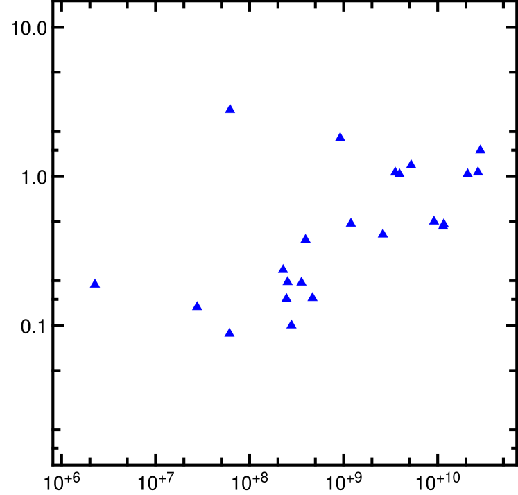
Figure 5: The radius of the sphere of influence $r_{\rm a}$ in arcsec as a function of black hole mass.

4.2 Keplerian regime

The criticism that $r_{\rm a}$ is often comparable with the resolution limit of the observations in question (Rix 1993) is no longer valid. This has been pointed out by Kormendy (1994), and we support his view with our carefully calculated values of $r_{\rm a}$ in the sense that the measured values do not cluster around any particular value (Table 1 and Figure 5). On the other hand, some of the smallest black holes have $r_{\rm a}$ comparable to or smaller than $0.1"$.

The black hole masses measured by Magorrian et al. (1998) required detailed modelling of the kinematics of the surrounding galactic nuclei. In principle one should see at small radius the Keplerian regime in which $\sigma^{2}\sim{M}/r$. This would be a very clear signature of a black hole, giving directly the mass to within a factor of order unity. The Keplerian regime should occur within some radius of order $r_{\rm a}$. We find that the logarithmic slope of $\sigma^{2}$ reaches $-0.95$ at a radius $r_{\rm K}$ which is generally much less than $r_{\rm a}$, with median value $\approx 0.2r_{\rm a}$ (this is of course consistent with the fact so much modelling had to be done to measure the black hole masses). This situation is also seen in the centre of the Milky Way, where the Keplerian regime is now resolved (Genzel et al. 1996) at $r_{\rm K}\sim r_{\rm a}/10$.

One might expect that the galaxies with the largest values of $r_{\rm K}$ would have the most secure black hole detections, but this appears not to be the case. The three galaxies where we find that $r_{\rm K}>0.5"$ are NGC 4486B, NGC 7768 and M31, and these do not appear to have significantly better black hole masses than any of the others.

5 Discussion

Note that the scaling relations of FR and CK giving ${\dot{N}}$ in terms ${M}$, $\rho_{0}$ and $r_{0}$ apply only in very specific circumstances. The result of CK only applies to the case ${r_{\rm crit}}<r_{\rm a}$. If ${r_{\rm crit}}<r_{\rm a}$ and $p\approx 1.8$ for $r<r_{\rm a}$ then CK equation (66) can be used to calculate ${\dot{N}}$, replacing $\rho_{0}\to\rho(r_{\rm a})$ and $r_{0}\to r_{\rm a}$, with the result roughly independent of what happens at $r>r_{\rm a}$. FR are careful to distinguish between the cases ${r_{\rm crit}}\grole r_{\rm a}$, and in these cases they use $p=7/4$ or $p=0$ accordingly. It is straightforward to generalise their expressions using equations (19) and (18).

Rauch & Tremaine (1997) have discussed the enhancement of tidal disruption rates by a process they call ‘resonant relaxation’. This effect can increase tidal disruption rates of stars which are bound to the black hole (i.e. at $r<r_{\rm a}$) by factors of order unity. Detailed calculations by Rauch & Ingalls (1997) also show that the effect is also quencehed by relativistic precession for black hole masses ${M}\ga 10^{8}{M_{\sun}}$. In the models we constructed the fuelling rate was never dominated by strongly bound stars, so in common with Rauch & Ingalls (1997), we find that resonant relaxation has little effect on tidal disruption rates.

There have been some observations of active galaxies which develop a broad-lined feature in their spectrum over a period of the order of months (Storchi-Bergmann et al. 1995, Eracleous et al. 1995). Eracleous et al. (1995) constructed a phenomonological model of such an event which involved an elliptical accretion disc, and suggested that such a disk could arise from the tidal disruption of a star (see also Syer & Clarke 1992). The size of the disc they required to fit the observations was too large to correspond to a main sequence disruption. It could, however, arise from the disruption of a red giant. Our discussion in Section 4.1 concluded that red giant disruptions with such short timescales should be very rare, so it is perhaps not surprising that such events are not encountered frequently.

References

- [1] Bahcall, J.N., & Wolf, R.A. 1976, ApJ, 209, 214
- [2]
- [3] Binney, J., and Tremaine, S. 1987, Galactic Dynamics, Princeton: Princeton University Press.
- [4] Bressan, A., Fagotto, F., Bertelli, G., & Chiosi, C. 1992, AA Supp., 100, 647
- [5]
- [6] Byun, Y.I., et al., 1996, AJ, 111, 1889
- [7]
- [8] Cannizzo, J.K., Lee, H.M., & Goodman, J. 1990, ApJ, 351, 38
- [9]
- [10] Cohn, H., & Kulsrud, R.M., 1978, ApJ, 226, 1087
- [11] Evans, C.R., & Kochanek, C.S. 1989, ApJ, 346, L13
- [12]
- [13] Fabian, A.C., Lee, J.C., Brandt, W.N., Iwasawa, K., & Reynolds, C.S., 1998, preprint (astro-ph/9803075).
- [14] Frank, J., & Rees, M.J. 1976, MNRAS, 176, 633
- [15]
- [16] Genzel, R., Hollenbach, D.J., Townes, C.H., Kroker, H., & Tacconi-Garman, L.E. 1996, ApJ, 440, 619
- [17]
- [18] Gerhard, O.E. & Binney J. 1985, MNRAS, 216, 467
- [19]
- [20] Haehnelt, M.G., & Rees, M.J. 1993, MNRAS, 263, 168
- [21]
- [22] Hill, J.G. 1975, Nature, 254, 295
- [23]
- [24] Lee, H., Kang, H., & Ryu, D. 1996, ApJ, 464, 131
- [25]
- [26] Joss, P. C., Rappaport, S., and Lewis, W. 1987, ApJ, 319, 180
- [27]
- [28] Kormendy, J. 1994, in The Nuclei of Normal Galaxies ed. Genzel, R. & Harris, A.I., (NATO ASI Ser. C., 445) (Dordrecht: Kluwer), p. 379.
- [29] Kormendy, J., & Richstone, D., 1995, ARAA, 33, 581
- [30]
- [31] Lasota, J.-P., Abramowicz, M. A., Chen, X., Krolik, J. Narayan, R., Yi, I. 1996, ApJ, 462, L142
- [32]
- [33] Lightman, A.P., & Shapiro, S.L. 1977, ApJ, 211, 244
- [34]
- [35] Magorrian, J., et al., 1998, AJ, 115, 2285
- [36]
- [37] Rauch, K.P., & Ingalls, B. 1997, preprint (astro-ph/9710288).
- [38] Rauch, K.P., & Tremaine, S. 1996, NewA, 1, 149
- [39]
- [40] Rees, M.J. 1998, Nature, 333, 523
- [41]
- [42] Reynolds, C.S, Di Matteo, T., Fabian, A. C., Hwang, U., & Canizares, C. R. 1996, MNRAS, 283, L111
- [43]
- [44] Reynolds, C.S, & Fabian, A.C., 1997, MNRAS, 290, 1
- [45]
- [46] Rix, H.-W., 1993, in IAU Symp. 153, Galactic Bulges, ed. Dejonghe & Habing, p. 423, Dordecht: Kluwer.
- [47] Schechter, P. 1976, ApJ, 203, 297
- [48]
- [49] Ulmer, A. 1997, ApJ, submitted, (astro-ph/9706247)
- [50]
- [51] Young, P.J., Shields, G.A., & Wheeler, J.C. 1977, ApJ, 212, 367
- [52]