Constraining $(\Omega,\Lambda)$ from weak lensing in clusters: the triplet method.

Abstract

We present a new geometrical method which uses weak gravitational lensing effects around clusters to constrain the cosmological parameters $\Omega$ and $\Lambda$ .
On each background galaxy, a cluster induces a convergence and a shear terms, which depend on the cluster projected potential, and on the cosmological parameters ($\Omega$, $\Lambda$), through the angular distance ratio $D_{LS}/D_{OS}$. To disentangle the effects of these three quantities, we compare the relative values of the measured ellipticities for each triplet of galaxies located at about the same position in the lens plane, but having different color redshifts. The simultaneous knowledge of the measured ellipticities and photometric redshifts enable to build a purely geometrical estimator (hereafter the $G(\Omega,\Lambda)$-estimator) independently of the lens potential.
More precisely $G$ has the simple form of the discriminant of a 3-3 matrix built with the triplet values of $D_{LS}/D_{OS}$ and observed ellipticities. $G$ is then averaged on many triplets of close-galaxies, giving a global function of ($\Omega$, $\Lambda$) which converges to zero for the true values of the cosmological parameters.
The linear form of $G$ regarding the measured ellipticity of each galaxy implies that the different noises on $G$ decrease as $1/\sqrt{N}$, where $N$ is the total number of observed distorted galaxies. A calculation and comparison of each source of statistical noise is performed .
The possible systematics are analyzed with a multi-screen lensing model in order to estimate the effect of perturbative potentials on galaxy triplets. Improvements are then proposed to minimize these systematics and to optimize the statistical signal to noise ratio.
Simulations are performed with realistic geometry and convergence for the lensing clusters and a redshift distribution for galaxies similar to what is observed. They lead to the encouraging result that a significant constraint on ($\Omega$, $\Lambda$) can be reached : $\Lambda_{-0.2}^{+0.3}$ in the case $\Omega+\Lambda=1$ or $\Omega_{-0.25}^{+0.3}$ in the case $\Lambda=0$ (at a 1$\sigma$ confidence level). In particular the curvature of the Universe can be directly constrained and the $\Omega=0.3$ and $\Omega=1$ universes can be separated with a 2$\sigma$ confidence level. These constraints would be obtained from the observations of nearly 100 clusters. This corresponds to about 20 nights of VLT observations.The method is still better adapted to a large program on the NGST. Hence, in complement to the supernovae method, the triplet method could in principle clear up the issue of the existence and value of the cosmological constant

Key words: cosmology – gravitational lensing – galaxies: clusters – dark matter

1 Introduction

Determination of the cosmological parameters of the standard cosmological models is one of the great challenge for the next ten years. Though these are the main objectives of the MAP and Planck Surveyor satellites, considerable efforts are devoted to the measurements of the ($\Omega$, $\Lambda$) parameters prior to the launch of these surveyors. In this respect, the supernovae search (see the Supernova Cosmological Project, Perlmutter et al. 1998) or gravitational lensing surveys (for a review see Mellier 1998) offer the best perspectives. In particular, if they are used jointly, a reasonable precision can be reached, provided that the degeneracy regarding to the determination of parameters $(\Omega,\Lambda)$ of each method are orthogonal. This is for instance the case for the supernovae experiments and the weak lensing analysis as presented hereinafter or as produced by large scale structures (Van Waerbeke et al 1998).
The limitations of any of these methods (even Planck measurements) are the understanding of the systematic bias and eventually the control of the large number of free parameters attached to each of them. Due to the difficulties to handle these issues it is important to diversify the methods to measure $(\Omega,\Lambda)$ and to find out some new observational tests. In this regard, any new method that controls properly its own systematics and that decreases the number of sensitive parameters needs careful attention.
It is well known that gravitational lensing can provide purely geometrical tests of the curvature of the Universe. Applications of this property to lensing clusters have been proposed by Breimer & Sanders (1992) and Link & Pierce (1998). They suggest to use giant arcs having different redshifts to probe directly the curvature of the Universe. Evidently this method can provide the cosmological parameters in the simplest way, provided that the modeling of the lens is perfectly constrained. Besides, it requires the spectroscopic redshifts of at least two different arcs in the same clusters, which is not an easy task. As such, this is a method which applies to very few clusters.
Fort, Mellier & Dantel-Fort (1996) focused on a statistical approach which explores the magnification bias coupled with the redshift distribution of the sources. Fort et al. use the shape and the extension of the depletion curves produced by the magnification of the galaxies to constrain the cosmological parameters and the redshift of the sources simultaneously. The intrinsic degeneracy can be somewhat broken if the redshift of a giant arc is known and if the number density of high-redshift background galaxies is significant. However, in practice, reliable results need the investigation of a significant number of lensing arc-clusters in order to improve the statistics, to minimize the systematics (like multiple lens planes) and to explore the sensitivity to the lens modeling.
The key issue on the Fort et al. approach is the coupling between the cosmological parameters, the redshift of the sources and the lens modeling. An attempt to disentangle these three quantities has been proposed by Lombardi & Bertin (1998), using a method which applies in rich clusters of galaxies, inside the region where the weak-lensing regime is valid. They use the knowledge of the photometric redshifts for a joint iterative reconstruction of the mass of the cluster and the cosmology. However their iteration method assumes that the mass of the deflecting cluster is known (or equivalently they assume that the mass-sheet degeneracy inherent to the mass reconstruction is broken). This assumption is the key of the problem, because it means that a perfect correction of the systematic bias on the $(\Omega,\Lambda)$ determination due to the systematic errors in the mass reconstruction (see section 3.1) can be achieved, which is still not presently the case (see Mellier 1998 for a comprehensive review). Indeed, for such a curvature test one should try to escape to the uncertainties of the potential modeling (mass reconstruction)of the cluster.
The triplet method proposed in this paper can solve this problem because it is based on the construction of an ($\Omega$,$\Lambda$)-estimator independent of the lens potential. Basically, it consists in comparing the elliptical shear of 3 nearby galaxies of different color redshifts probing the same part of the potential across the cluster. When the galaxies are close enough, their observed ellipticity only depends on three unknown parameters, the local convergence and shear (related to the second order derivatives of the projected potential of the cluster) and namely the cosmological parameter ($\Omega,\Lambda$), through the angular distance ratio $D_{LS}/D_{OS}$. The use of a triplet of nearby galaxies enables to break this degeneracy and provides a local geometrical operator only dependent on ($\Omega,\Lambda$). We chose a local linear operator regarding to the observed ellipticities, and we average it on all set of close-triplets detected in many lens planes. Follows a global geometrical estimator, biased by a noise (coming mainly from the intrinsic source ellipticities) which decreases as the inverse of the square root of the number of triplets. It means that with a large number of lensing clusters one can estimate ($\Omega,\Lambda$) with a reasonable accuracy. This technique and its efficiency are discussed in the following sections.
Section 2 reminds rapidly the lensing equations and the basic lensing quantities relevant for the paper. Section 3 shows how to build the geometrical estimator $G$ which uses triplets of distorted galaxies. The principle and the detailed analysis of our method are also discussed. The signal to noise ratio of the method is then derived as well as the probability distribution of the cosmological parameters ($\Omega$,$\Lambda$). Although the main objective of this first paper is mostly to present the principle of the method, Section 4 gives an evaluation of the amplitude of several systematic biases coming from possible perturbing lenses distributed along the line of sight of triplets (galaxies or larger structures). Preliminary solutions to these systematic biases and ideas of optimizing the method (Selection in the geometry of clusters and choice of redshifts) are developed in section 5. The method is tested on simulations in Section 6. Finally, we discuss the results and suggest some observational strategies in Section 7.

2 The weak lensing equations

The lensing properties are determined by the dimensionless convergence (the strength of the lens) $\kappa$ and shear (the distortion induced by the lens) $\gamma$, which both depend on the second order derivatives of the two-dimensional projected deflecting potential. The lensing effect of a cluster on background galaxies can be expressed as an amplification matrix defined in each angular position around the cluster as (Schneider et al. 1992)

$$A^{-1} = \left(\begin{array}[]{lr}1-\kappa-\gamma_{1}&-\gamma_{2}\\ -\gamma_{2}&1-\kappa+\gamma_{1}\end{array}\right)\ ,$$ (3)

where

$$\mbox{\boldmath$\gamma$}=\gamma_{1}+i\gamma_{2}.$$ (4)

$\kappa$ is a dimensionless form of the cluster surface mass density $\Sigma$ :

$$\kappa=\Sigma/\Sigma_{crit}\ \mbox{with}\ \Sigma_{crit}=\frac{c^{2}}{4\pi GD_{OL}}\frac{D_{OS}}{D_{LS}}\ ,$$ (5)

where $D_{OS}$, $D_{OL}$ and $D_{LS}$ are the angular diameter distances from the observer to the source, from the observer to the lens and from the lens to the source respectively. For the weak lensing regime the gravitational distortion produced by a lensing cluster can be modeled by a transformation in the ellipticity of the galaxies from the source plan ($\epsilon_{S}$) to the image plane ($\epsilon$) (see Appendix A) :

$$\mbox{\boldmath$\epsilon$}=(1-g^{2})\mbox{\boldmath$\epsilon$}_{S}+\mbox{\boldmath$g$}=\bar{\mbox{\boldmath$\epsilon$}}_{S}+\mbox{\boldmath$g$}\ \mbox{\ \ with\ \ }\ \mbox{\boldmath$g$}=\frac{\mbox{\boldmath$\gamma$}}{1-\kappa}.$$ (6)

$\epsilon$ is the complex observed ellipticity, $g$ is the complex reduced shear and $\bar{\mbox{\boldmath$\epsilon$}}_{S}$ is what we will call the complex corrected source ellipticity. Either in the source or the image plan, the ellipticity parameter is defined by :

$$\mbox{\boldmath$\epsilon$}=\epsilon\ e^{2i\theta}\ \mbox{with}\ \epsilon=\frac{1-r}{1+r};$$ (7)

$r$ is the axis ratio of the image isophotes and $\theta$ is the orientation of the main axis.
The convergence and the shear both depend on the source redshift through an absolute lensing factor $\omega_{a}$ appearing in equation (3) :

$$\omega_{a}(z)=\frac{D_{LS}}{D_{OS}}\ .$$ (8)

Adopting the notation of Seitz & Schneider (1997) who relate the lensing parameters to the value they would have at infinite redshift, $\kappa$ and $\gamma$ now write :

$$\kappa = \omega(z)\kappa_{\infty}\ ,$$ (9)

$$\gamma = \omega(z)\mbox{\boldmath$\gamma$}_{\infty}\ ,\ {\rm where}$$ (10)

$$\omega(z) = \frac{\omega_{a}(z)}{\omega_{a}(\infty)}\ .$$ (11)

Hereafter, $\omega(z)$ will be named the lensing factor. This is the term which contains the cosmological dependency.

3 The method

The behavior of $\omega(z)$ with $\Omega$ in the case $\Omega+\Lambda=1$ (flat geometry) and in the case $\Lambda=0$, is given on figure (1). All curves range from $0$ (for a source redshift equal to the cluster redshift) to $1$ (for an infinite source redshift). Their main difference is a small change in their convexity. That is why the use of numerous triplets of sources at different redshifts may disentangle these curves, i.e. provide a constraint on the cosmological parameters.

Fig. 1.: $\omega$ versus redshift in the cases $\Omega+\Lambda=1$ and $\Lambda=0$, for a cluster lying at a redshift $0.4$. Different curves correspond to $\Omega=$ $0.2$ (bottom curve), $0.4,0.6,0.8$ and $1.0$ (top curve). All curves start from $0$ (at redshift $0.4$) and converge to $1.0$ when the redshift becomes infinite. The triplet method applies to their different relative convexity.

The core of the method is to proceed in such a way that this constraint is independent on the potential of the cluster. We have constructed an operator which depends theoretically on ($\Omega,\Lambda$) and can be computed simply from the observed ellipticities of background galaxies as well as their photometric redshift. Its main property is to be equal to zero when the cosmological parameters are equal to the actual ones. We proceed in two steps: first, we build such an operator ($G_{ijk}$) from triplets of close sources, and second we average it on many triplets of sources to obtain the final geometrical operator $G$.

3.1 Construction of $G_{ijk}$

For a background galaxy at redshift $z_{i}$, equation (4) rewrites

$$\mbox{\boldmath$\epsilon$}_{i} = \bar{\mbox{\boldmath$\epsilon$}}_{S,i}+\mbox{\boldmath$g$}_{i}^{o}\ \mbox{with}$$ (12)

$$\mbox{\boldmath$g$}_{i}^{o} = \frac{\omega_{i}^{o}\mbox{\boldmath$\gamma$}_{\infty}}{1-\omega_{i}^{o}\kappa_{\infty}},$$ (13)

where the lower index ($i$) refers to the redshift $z_{i}$ and the upper index (^o) refers to the actual values of the cosmological parameters : $\Omega_{o}$,$\Lambda_{o}$. The second term in equation (10), $\mbox{\boldmath$g$}_{i}^{o}$ represents the part of the image ellipticity that depends on the cosmology.
Let us now consider a triplet of background neighboring galaxies in the image plane and lying at redshifts $z_{i}$, $z_{j}$ and $z_{k}$. The number density of triplets depends on the deepness of the observations. For instance, up to $R=26$ mag., we expect a mean density of $50$ sources arcmin^-2, that is about 4 sources inside a circle of radius $10$ arcseconds. In the following, we thus consider that each galaxy of the triplet is distorted by the same local potential i.e. $\kappa_{\infty}$ and $\mbox{\boldmath$\gamma$}_{\infty}$ are the same for the three galaxies. The bias induced by this approximation will be discussed in section 3.4. The triplet of galaxies gives a triplet of equations (11) respectively indexed by $i$, $j$ and $k$ from which we can derive a final equation independent both on $\kappa_{\infty}$ and $\mbox{\boldmath$\gamma$}_{\infty}$. This equation writes simply as the zero of a 3-3 determinant :

$$\left|\begin{array}[]{lcr}1&\omega_{i}^{o}&\omega_{i}^{o}g_{j}^{o}g_{k}^{o}\\ 1&\omega_{j}^{o}&\omega_{j}^{o}g_{k}^{o}g_{i}^{o}\\ 1&\omega_{k}^{o}&\omega_{k}^{o}g_{i}^{o}g_{j}^{o}\\ \end{array}\right|=0\ .$$ (17)

The first term of this equation can now be formally generalized to a complex operator $G_{ijk}$ of $(\Omega,\Lambda)$ built from the complex measured ellipticities of the three galaxies :

$$G_{ijk}(\Omega,\Lambda)=\left|\begin{array}[]{lcr}1&\omega_{i}&\omega_{i}\mbox{\boldmath$\epsilon$}_{j}\par\mbox{\boldmath$\epsilon$}_{k}^{*}\\ 1&\omega_{j}&\omega_{j}\mbox{\boldmath$\epsilon$}_{k}\par\mbox{\boldmath$\epsilon$}_{i}^{*}\\ 1&\omega_{k}&\omega_{k}\mbox{\boldmath$\epsilon$}_{i}\par\mbox{\boldmath$\epsilon$}_{j}^{*}\\ \end{array}\right|\ .$$ (21)

The dependency in $(\Omega,\Lambda)$ is contained in each term $\omega_{s}(\Omega,\Lambda)$ ($s=i$, $j$ or $k$) defined by equation (9) for $z=z_{s}$. $G_{ijk}$ is more explicitly the sum of two $(\Omega,\Lambda)$ functions: $G_{ijk}^{main}$ which is equal to zero for the actual values of the cosmological parameters, and a complex noise $N$:

$$G_{ijk}=G_{ijk}^{main}+N\ ,$$ (22)

where

$$G_{ijk}^{main} = \left|\begin{array}[]{lcr}1&\omega_{i}&\omega_{i}/\omega_{i}^{o}\\ 1&\omega_{j}&\omega_{j}/\omega_{j}^{o}\\ 1&\omega_{k}&\omega_{k}/\omega_{k}^{o}\\ \end{array}\right|\omega_{i}^{o}\omega_{j}^{o}\omega_{k}^{o}\ \gamma_{\infty}^{2}.$$ (26)

At this point it is important to stress that the $\kappa_{\infty}$ contribution cannot be neglected (see equation (11)). Indeed, if we consider for instance a $0.1$ variation of the cosmological parameters (along the gradient of $\omega(\Omega,\Lambda)$), the resulting relative variation of the term $\omega\gamma$ is about $1\%$ which is about ten times smaller than the relative variation due to the $1-\omega\kappa$ term, in equation (11). That is why both contributions from the local convergence ($\kappa_{\infty}$) and the local shear ($\gamma_{\infty}$) of the cluster potential must be taken in account.
Lombardi & Bertin (1998) proposed to reconstruct jointly the shear, the convergence and $(\Omega,\Lambda)$ in the weak lensing area, with an iteration method based on the equation (11). Their method seems to converge relatively rapidly with a small number of clusters but it seems that for their simulations they implicitly assume that the mass of the cluster is known. However, one can see that equation (11) is invariant when replacing $\gamma_{\infty}$ by $\alpha\gamma_{\infty}$ and $1-\omega\kappa_{\infty}$ by $1-\alpha\omega\kappa_{\infty}$ ($\alpha$ is a constant). This expresses the mass-sheet degeneracy problem which implies that the total mass of the lensing cluster is uncertain. Indeed, despite the numerous suggestions which have been proposed in order to solve this issue (Seitz & Schneider, 1997), for the moment mass reconstruction techniques cannot disregard systematic errors analysis (see Mellier 1998 for a comprehensive review). As an example, a $20\%$ systematic bias on the determination of the total mass of the cluster (or equivalently a $20\%$ systematic on the mean value of $\kappa_{\infty}$) is equivalent to a systematic bias larger than 0.2 on the value of the cosmological parameters (when compared to the $1\%$ contribution from the lensing factor mentioned above). Therefore, the knowledge of the lens potential is a critical strong assumption.
In the triplet method it is possible to constrain the cosmological parameters regardless the potential of the lens. No assumption is made in order to relate the values of the local shear and the local convergence. Hence they are considered as independent parameters. In order to construct a $G$ operator which only depends on $(\Omega,\Lambda)$, we then need three local equations relating $\kappa_{\infty}$, $\gamma_{\infty}$ and $(\Omega,\Lambda)$ to cancel the potential dependency. This is achieved with the measured ellipticity equations (10) applied to triplets of close galaxies at different redshifts. Besides, the form of the $G$ operator becomes unique and must have the formal expression given in equation (13) if we want it linear with respect to the ellipticities provided by the observations. To sum up, the use of triplets of galaxies through the operator $G$ is the simplest way to build a pure geometrical operator which drops both the $\kappa_{\infty}$ and $\gamma_{\infty}$ dependencies and keeps linear regarding to the ellipticities.

The statistical noise $N$ will be more explicitly calculated in section 3.4. For the moment it is just important to understand that the probability distribution of this noise (real and imaginary parts) regarding the different triplets of galaxies is a random law centered on 0 since the linear construction of $G$ makes the different sources of noise (mainly the intrinsic source ellipticity) be randomly distributed around 0.
The above formula does not take in account the systematics (an effect of galaxy-galaxy lensing, a presence of background structures) that will be studied further in section 4.

3.2 Construction of $G$

Before averaging $G_{ijk}(\Omega,\Lambda)$ on many triplets (that is to say on all the triplets done with galaxies contained within a given radius), let us stress that it makes sense. Indeed, by averaging (we only consider the real part of the complex noise) on many triplets the noise contribution decreases as $1/\sqrt{N}$, with $N$ the number of background galaxies (and not the number of triplets, since many triplets are redundant). While the noise is vanishing, the method can provide valuable constraints as far as cosmological operator $G_{ijk}^{main}$ does not vanish too, or in other words if its behavior with $\Omega$ and $\Lambda$ is the same (not random) whatever the triplet is. Fortunately this is the case provided that the three redshifts of all the triplets are ordered similarly : for example $z_{i}<z_{j}<z_{k}$.
Consequently we can derive $G$ from an average of $G_{ijk}$ on all the ordered triplets ${ijk}$ :

$$G(\Omega,\Lambda)=<G_{ijk}>_{(i<j<k)}\ .$$ (27)

According to equation (14), $G$ is also composed of two terms : the first one $G^{main}$ which has the same properties as $G_{ijk}^{main}$, and a Gaussian noise $GN$ which decreases as $1/\sqrt{N}$,

$$R_{e}(G)(\Omega,\Lambda)=G^{main}(\Omega,\Lambda)+Re(GN)\ ,$$ (28)

where

$$G^{main}=\left<\left|\begin{array}[]{lcr}1&\omega_{i}&\omega_{i}/\omega_{i}^{o}\\ 1&\omega_{j}&\omega_{j}/\omega_{j}^{o}\\ 1&\omega_{k}&\omega_{k}/\omega_{k}^{o}\\ \end{array}\right|\omega_{i}^{o}\omega_{j}^{o}\omega_{k}^{o}\right>_{(ijk)}\left<\gamma_{\infty}^{2}\right>\ ,$$ (32)

and

$$R_{e}(GN)\propto 1/\sqrt{N}\ ,$$ (33)

where $R_{e}$ denotes the real part of the complex quantities. $<\gamma_{\infty}^{2}>$ is the square of $\gamma_{\infty}$ averaged on the weak lensing area. We consider the real part of $G$ ($Re(G)$) because as $N$, the noise $GN$ is complex.
By construction $G^{main}$ is equal to zero at the position ($\Omega_{o}$, $\Lambda_{o}$). We thus can write the following equation (biased by the presence of the Gaussian noise) which sums up the method : ($\Omega_{o}$, $\Lambda_{o}$) is a solution of

$$G(\Omega,\Lambda)\equiv 0.$$ (34)

In order to see if the triplet method can be effective from the observational point of view two questions have to be addressed:

1. how is the $G$-operator degenerated in $(\Omega,\Lambda)$?

2. how many clusters are necessary to cancel the noise contribution with respect to the cosmological information contained in $G^{main}$ ?

3.3 The main cosmological term: $G^{main}(\Omega,\Lambda)$

Figure (2) gives the contours of $G^{main}/<\gamma_{\infty}^{2}>$ in the $(\Omega,\Lambda)$ plan, for the redshift distribution (42), as taken in the simulations (see section 6). From this graph we see that the method is degenerated in $(\Omega,\Lambda)$. The degeneracy is parallel to the $G$-contours. To break this degeneracy one has either to make a theoretical assumption (for example $\Omega+\Lambda=1$ ) or to add another experimental degenerated constraint which contours are as orthogonal to the $G$-contours as possible, like for example high-redshift supernovae (Perlmutter et al. 1998). Considering the mean orientation of its degeneracy, the triplet method can also be seen as a direct measure of the curvature of the Universe $1-\Omega-\Lambda$.
From figure (2) we also get quantitatively the variations of $G$. It shows that, for an accuracy of about $10\%$ on the cosmological parameters (along the gradient of $G$), we must obtain a precision of about $10^{-4}<\gamma_{\infty}^{2}>$ on G. This rate of variation has to be compared with the noise on $G$.

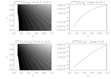
Fig. 2.: Contours of $G^{main}(\Omega,\Lambda)/<\gamma_{\infty}^{2}>$ in the cases $(\Omega,\Lambda)=(0.3,0.7)$ (top panel) and $(0.3,0)$ (bottom panel). The right part of the figure gives the restriction of $G^{main}$ to the particular domains $\Omega+\Lambda=1$ (top) and $\Lambda=0$ (bottom).

3.4 Noise on G

The complex noise is produced by four sources:

1. noise from the corrected source ellipticities $\bar{\epsilon}_{S,i,j,k}$,

2. the errors propagation on the measured ellipticities $\Delta\epsilon_{i,j,k}$ (it behaves similarly as the previous ones),

3. the three sources do not have the same $\gamma_{\infty}$ and we thus have to consider $\Delta\gamma_{\infty,i,j,k}$ (in other words , each source, though close to each other, do not exactly cross the potential at the same position),

4. the photometric redshifts are not the true redshifts and lead to shifts $\Delta\omega_{i,j,k}$ on the lensing factors.

From equations (13) it is clear that, due to the linearity of the 3-3 determinant and of the averaging on all the triplets, the final noise is linear regarding to each individual term : it is composed to first order of linear combination of terms (like $\bar{\epsilon}_{S,i}$), and to second order of linear combination of crossed-terms (like $\epsilon_{S,i}.\Delta\omega_{j}$). These crossed-terms cannot introduce any systematic bias on G and thus can be neglected.
The following equations give the four different noise contributions: $GN_{\epsilon_{S,i}}$, due to the corrected source ellipticity, $GN_{\Delta\epsilon_{i}}$, due to the error on the ellipticity, $GN_{\Delta\omega_{i}}$ due to the approximate redshift and $GN_{\Delta\gamma_{\infty,i}}$ due to the potential,

$$GN_{\bar{\epsilon}_{S,i}}\simeq<\gamma_{\infty}^{2}> <\omega_{j}\omega_{k}^{o}(\omega_{i}-\omega_{k})\bar{\mbox{\boldmath$\epsilon$}}_{S,i}^{*}/\mbox{\boldmath$\gamma$}^{*}$$

$$+\omega_{j}^{o}\omega_{k}(\omega_{j}-\omega_{i})\bar{\mbox{\boldmath$\epsilon$}}_{S,i}/\mbox{\boldmath$\gamma$}>$$

$$GN_{\Delta\epsilon_{i}}\simeq<\gamma_{\infty}^{2}> <\omega_{j}\omega_{k}^{o}(\omega_{i}-\omega_{k})\Delta\mbox{\boldmath$\epsilon$}_{i}^{*}/\mbox{\boldmath$\gamma$}^{*}$$

$$+\omega_{j}^{o}\omega_{k}(\omega_{j}-\omega_{i})\Delta\mbox{\boldmath$\epsilon$}_{i}/\mbox{\boldmath$\gamma$}>$$

$$GN_{\Delta\omega_{i}}\simeq<\gamma_{\infty}^{2}> <\Delta\omega_{i}(\omega_{j}\omega_{k}^{o}(\omega_{k}-\omega_{j})$$

$$+\omega_{j}\omega_{k}^{o}\omega_{i}^{o}-\omega_{j}^{o}\omega_{k}\omega_{i}^{o})>$$

$$GN_{\Delta\gamma_{\infty,i}}\simeq<\gamma_{\infty}^{2}> <\omega_{j}\omega_{k}^{o}(\omega_{i}-\omega_{k})\Delta\mbox{\boldmath$\gamma$}_{i}^{*}/\mbox{\boldmath$\gamma$}^{*}$$

$$+\omega_{j}^{o}\omega_{k}(\omega_{j}-\omega_{i})\Delta\mbox{\boldmath$\gamma$}_{i}/\mbox{\boldmath$\gamma$}>.$$

The terms of index $j$ and $k$ can be easily derived from these equations by cyclic permutations of the ($ijk$) triplet.
It is worth noting that even if the bias, as $G^{main}$, is a function of the cosmological parameters, we can neglect this dependency. Indeed, for a given shift of $(\Omega,\Lambda)$ around $(\Omega_{o},\Lambda_{o})$ the variations of $G^{main}$ and $GN$ verify $\Delta R_{e}(GN)/\Delta G^{main}\propto 1/\sqrt{N}$. Besides, provided that $N$ is large enough, the probability distribution of the noise $R_{e}(GN)$ can be considered as a Gaussian law centered on 0 (as the sum of a large number of nearly Gaussian laws). So far, we have shown that the variance of this noise decreases as $1/\sqrt{N}$ because of the redundancy of triplets. This applies for $GN_{\bar{\epsilon}_{S,i}}$, $GN_{\Delta\epsilon_{i}}$ and $GN_{\Delta\omega_{i}}$ but not for $GN_{\Delta\gamma_{\infty,i}}$. Indeed, for a galaxy $i$ included in two different triplets the associated term $\Delta\mbox{\boldmath$\gamma$}_{i}$ is different in each triplet. That is why the variance of the fourth noise $GN_{\Delta\gamma_{\infty,i}}$ vanishes in $1/\sqrt{3N_{tr}}$, where $N_{tr}$ is the total number of triplets : $N_{tr}\approx 3N$ (see the remark of section 3.1).
The variances of the four noises behave approximately as follows (under the conditions that will be detailed in section 6) :

$$GN_{\bar{\epsilon}_{S,i}} \approx 0.08\frac{<\gamma_{\infty}^{2}>}{\sqrt{N}}\ ,$$ (39)

$$GN_{\Delta\epsilon_{i}} \approx 0.02\frac{<\gamma_{\infty}^{2}>}{\sqrt{N}}\ ,$$ (40)

$$GN_{\Delta\omega_{i}} \approx 0.04\frac{<\gamma_{\infty}^{2}>}{\sqrt{N}}\ ,$$ (41)

$$GN_{\Delta\gamma_{\infty,i}} \approx 0.02\frac{<\gamma_{\infty}^{2}>}{\sqrt{N}}\ ,$$ (42)

3.5 Resulting signal to noise ratio

Let us establish the relation between the signal to noise ratio of the method and the number of background galaxies (or the number of considered clusters). In the following we will take only $1000$ galaxies per cluster (see section 6). If we define the signal as a variation of $G^{main}$ along its gradient and $\sigma_{GN}$ as the variance of the statistical noise (see section 3.4), the signal to noise ratio can thus be written as :

$$S/N=\frac{\Delta G^{main}}{\sigma_{GN}}=\frac{\Delta_{\Omega,\Lambda}\left|\left|\mathchoice{\mbox{\boldmath$\displaystyle\bigtriangledown$}}{\mbox{\boldmath$\textstyle\bigtriangledown$}}{\mbox{\boldmath$\scriptstyle\bigtriangledown$}}{\mbox{\boldmath$\scriptscriptstyle\bigtriangledown$}}G^{main}_{\mid\Omega_{o},\Lambda_{o}}\right|\right|}{\sigma_{GN}}.$$ (43)

The $\left|\left|...\right|\right|$ notation indicates the norm of a vector. $\Delta_{\Omega,\Lambda}$ is the accuracy on the cosmological parameters. Figure (3) plots the variation of $\Delta_{\Omega,\Lambda}$ as a function of the number of clusters (with an observed number density of background galaxies equal to $50$ by square-arcminute) for a $1\sigma$ confidence level. This plot shows that an accuracy of $0.1$ can be reached (at a $1\sigma$ level) with about 1000 clusters, or similarly an accuracy of about $0.3$ can be reached (at a $1\sigma$ level) with $100$ clusters.
It shows that with a good seeing one could in principle test the existence of a cosmological constant from VLT observations with about 100 clusters. Far better it should be possible to measure the curvature of the Universe with a reasonable accuracy from NGST observations (the number density of background galaxies is multiplied by 10). These prospects of course require that the systematics are previously corrected.

Fig. 3.: Accuracy on the cosmological parameters versus the number of clusters (with $1000$ galaxies per cluster) at a $1\sigma$ confidence level. The plain line extrapolates the results obtained from simulations with an inverse square root function. Error bars account for the number of simulations. We can read that a $0.3$ accuracy (at $1\sigma$) can be achieved with the observations of $100$ clusters or a $0.1$ accuracy (at $1\sigma$) can be achieved with the observations of $1000$ clusters. Equivalently a $0.2$ accuracy (at $2\sigma$) can be achieved with the observations of $1000$ clusters.

These results can be refined by the introduction of a probability distribution.

3.6 The $(\Omega,\Lambda)$ probability distribution

Thanks to the Gaussian behavior of the noise we can derive from the operator $G(\Omega,\Lambda)$ a probability distribution $p(\Omega,\Lambda)$ for the cosmological parameters :

$${p_{\Omega,\Lambda}(\Omega,\Lambda)}\equiv\displaystyle{{\rm exp}\left(-{\left[R_{e}\left[G\left(\Omega,\Lambda\right)\right]\right]^{2}\over 2\sigma_{GN}^{2}}\right)}\ ,$$ (44)

which has just to be normalized on the considered domain of $(\Omega,\Lambda)$, (for example $\Omega+\Lambda=1$).
The operator $G(\Omega,\Lambda)$ is directly derived from the observational data. On the other hand, $\sigma_{GN}$ is obtained from simulations applied on the data in the following way. Once the function $G(\Omega,\Lambda)$ is obtained from the observation of ($\epsilon$, z), it is possible to add noise to the data by adding random ellipticities ($\mbox{\boldmath$\epsilon$}_{S}$) and $\Delta z$ random errors to the redshifts $z$ : the variance of the noise $GN$ induced on $G$ is then directly $\sigma_{GN}$.

4 Analysis of systematics

In this section we discuss the systematics which could potentially reduce significantly the efficiency of the method from an observational point of view. Though we give estimations of their amplitude, it is worth noting that a reliable quantitative estimate of their impact on the triplet method will demand additional work (mainly simulations and calculations taking in account the perturbation coming from large-scale structures. This effect will be studied in paper II).
Two main systematics have been identified:

1. a systematic bias on $G$ produced by to the non-symmetry of the term $\Delta\omega$. It can be easily corrected (see 4.1).
   

2. a contamination produced by the existence of background structures which play the role of perturbing lenses. They can be the background galaxies themselves (which induce galaxy-galaxy lensing) and possibly any condensation of mass (clusters or large-scale structures) located on the line of sight of the lensing cluster. In the following sections (section 4.2 and 4.3), we focus on two extreme cases: the systematic produced by the galaxies of each triplet themselves, and those generated by large-scale structures. This study will be performed using multi-lensing models (see Kovner 1987). Appendix B gives the calculation of the measured ellipticities in a multi-lensing model.

4.1 Non symmetry of the term $\Delta\omega$

The method supposes that we know the photometric redshifts of background galaxies as well as the probability distribution $p_{\Delta z}(\Delta z)$ of the error between the photometric redshift and the true one. Even if $p_{\Delta z}(\Delta z)$ is symmetric and centered on 0, which is not necessarily the case, the probability distribution of the resulting shift on $\omega$, $p_{\Delta\omega}(\Delta\omega)$ may be non symmetric and the mean value of $\Delta\omega$ may be different from zero, introducing a systematic in equation (23). Fortunately, this effect is easy to correct. Since the redshift distribution $n(z)$ is known the systematic can be exactly balanced by replacing in the definition of $G_{ijk}$ $\omega$ by $\omega-\overline{\Delta\omega}$, where

$$\overline{\Delta\omega}(z)=\int\omega(z+\Delta z)n(z+\Delta z)p_{\Delta z}(\Delta z)d\Delta z\ .$$ (45)

4.2 Potential perturbation due to galaxy-galaxy lensing

Since we consider triplets of galaxies having different redshifts but which are very close together in the image plane, the most distant can potentially be distorted by the lensing effect of the others. In particular, in each triplet ($i,j,k$) (ordered with increasing redshifts) the galaxy $i$ is a perturbation of the potential for the sources $j$ and $k$ as well as the galaxy $j$ for the source $k$. It is worth noting that $i$ is not the only perturbing lens for the source $j$, and $i$ and $j$ are not the only one for the source $k$. For instance, each galaxy may be itself part of a group of galaxies which produces its own additional lensing effect. Nevertheless, in order to get a rough estimate of the amplitude of this kind of systematics, we will assume to first approximation that the galaxy-galaxy lensing produced within each triplet, is the dominant contribution.
The galaxy-galaxy lensing increases as the angular distance between the galaxy-lens and the galaxy-source decreases. It also depends on their relative redshifts: that is why it induces a systematic bias on the construction of $G$. In Appendix B we compute the amplitude of the corrections on the measured ellipticities once several lenses along the line of sight are taken into account. From Equations (62), (63) and (66) of Appendix B, one can see that these perturbations produce two kinds of taxes:

1. A purely additive term, $g^{P}$. It can be seen as the linear contribution from the shear, as if the shears of each lenses were simply added to each other without coupling considerations.

2. A a multiplicative term of the form $\left(1-\left(1-c\right)\kappa^{P}\right)^{-1}$ which modifies the main cosmological term $g$. It accounts for couplings between the main and additional lenses.

4.2.1 The additive linear term.

Since the three galaxies of each triplet are randomly distributed and uncorrelated, this term induces a noise rather than a systematic bias. It decreases as $1/\sqrt{3N}$, like the noise $GN_{\Delta\gamma_{\infty}}$ for instance. Besides, the shear induced by a galaxy-lensed can be controlled (if we cancel the triplets where the angular distance between two of the three sources is too small: typically lower then a few arcsecond for typical Einstein radius of galaxies. This means an induced shear inferior to about $2\%$). Therefore the amplitude of this additive term can be bounded to less than $10\%$ of the effect coming from the principal statistical noise $GN_{\epsilon_{S,i}}$, and thus can be neglected.

4.2.2 The multiplicative coupling term.

The effect of coupling between two lenses depends on their relative redshifts through angular distances ratio, hence this term really induces a systematic bias on $G$. To calculate it we have to think about the meaning of the additional convergence, $\kappa^{P}$, used in the multi-lens screen approach of the annex B. This convergence associated to the source $j$ and produced by the galaxy-lens $i$ will be noted $\kappa^{i,j}$; the convergences associated to the source $k$ and produced by the galaxy-lenses $i$ and $j$ will be noted $\kappa^{i,k}$ and $\kappa^{j,k}$. We cannot directly compare their value since they depend on the redshifts $z_{i},z_{j},z_{k}$. So, in order to model this systematic bias we associate to each of these convergences an absolute one $\tilde{\kappa}^{gal}$ independent of the redshifts $z_{i}$, $z_{j}$ and $z_{k}$ (obviously $\tilde{\kappa}^{gal}$ should depend on the angular distance between the galaxy-source and the galaxy lens. We consider here a mean value averaged over the area around each galaxy-lens where we search for a source. For the definition of this area, see section 5.2):

$$\kappa^{i,j} = \frac{D_{Oi}}{D_{OL}}\frac{D_{ij}}{D_{Oj}}\tilde{\kappa}^{gal}$$ (46)

$$\kappa^{i,k} = \frac{D_{Oi}}{D_{OL}}\frac{D_{ik}}{D_{Ok}}\tilde{\kappa}^{gal}$$ (47)

$$\kappa^{j,k} = \frac{D_{Oj}}{D_{OL}}\frac{D_{jk}}{D_{Ok}}\tilde{\kappa}^{gal}.$$ (48)

The $\Delta_{\Omega,\Lambda}^{GGL}$ shift (along the gradient of $G$) on the cosmological parameters determination and due to the galaxy-galaxy lensing perturbation effects is then :

$$\frac{\left<\left|\begin{array}[]{lcr}1&\omega_{i}&0\\ 1&\omega_{j}&\frac{D_{ij}}{D_{OL}}(\frac{D_{Oi}}{D_{Oj}}-\frac{D_{Li}}{D_{Lj}})\\ 1&\omega_{k}&\frac{D_{ik}}{D_{OL}}(\frac{D_{Oi}}{D_{Ok}}-\frac{D_{Li}}{D_{Lk}})+\frac{D_{jk}}{D_{OL}}(\frac{D_{Oj}}{D_{Ok}}-\frac{D_{Lj}}{D_{Lk}})\\ \end{array}\right|\right>}{\left|\left|\mathchoice{\mbox{\boldmath$\displaystyle\bigtriangledown$}}{\mbox{\boldmath$\textstyle\bigtriangledown$}}{\mbox{\boldmath$\scriptstyle\bigtriangledown$}}{\mbox{\boldmath$\scriptscriptstyle\bigtriangledown$}}_{\Omega_{0},\Lambda_{0}}\left<\left|\begin{array}[]{lcr}1&\omega_{i}&\omega_{i}/\omega_{i}^{o}\\ 1&\omega_{j}&\omega_{j}/\omega_{j}^{o}\\ 1&\omega_{k}&\omega_{k}/\omega_{k}^{o}\\ \end{array}\right|\right>\right|\right|}\tilde{\kappa}^{gal}$$ (55)

where the brackets $\left<...\right>$ denote the average over all the ordered triplets.
Using the redshift distribution (42) and considering the mean value of the convergence created by a galaxy as about $2\%$ (see section 5.2), one gets : $\Delta_{\Omega,\Lambda}^{GGL}=10.2\tilde{\kappa}^{gal}\approx 0.2$.
This is only an indicative value. However, with galaxy/galaxy lensing measurements, we are in principle able to account for the effect of the potential of each background galaxy. This systematic can be calculated and corrected. Therefore, if the knowledge of the mean potential of galaxies can be reached with about a $\approx 20\%$ accuracy (we could use Faber-Jackson models or wait for the incoming results of galaxy-galaxy lensing studies (see Schneider et al. 1996)), the remaining systematic would then be about $\Delta_{\Omega,\Lambda}^{GGL}\approx 0.04/\sqrt{Nclust}$.
This correction does not take in account the possibility that a fraction of the galaxies are embedded in groups which could enhance the contamination. There are two possibilities to solve this issue. Since we know the photometric redshifts of the galaxies we can discriminate compact groups of galaxies and remove the corresponding triplets from the sample. Or, if the galaxy-galaxy lensing results are able to account for these effects with a reasonable accuracy, then we can as previously calculate $\Delta_{\Omega,\Lambda}^{GGL}$.
In conclusion this effect is non-negligible but can be accurately estimated and corrected, thanks to the forthcoming observations of galaxy-galaxy lensing on blank fields.

4.3 Potential perturbation due to background lensing structures

Let us consider the perturbation due to background structures. Before giving an estimate of it for the case of matter structures integrated along the line of sight, we calculate the perturbation due to a single lens plane (containing an over dense region like a cluster or even an under dense region). Since this second lens may be located anywhere in redshift then it differently affects the measured ellipticities of the sources ($i,j,k$) in each triplet, it can induce a systematic on the value of $G$. Once again and still using the calculations done in annex B (see equation (66)), this systematic can be split in two parts due to an additive term (corresponding to the linear contribution of the perturbative lens) and a multiplicative term (corresponding to the coupling between the main and the perturbative lenses).

4.3.1 The additive linear term.

Like in the above section, we associate an absolute convergence and shear $\delta\tilde{\kappa}$ and $\delta\tilde{\gamma}$ to the additional convergence and shear $\delta\kappa^{P,S}$ and $\delta\gamma^{P,S}$ coming from the lensing effect of the structure on a source S (S can be $i$, $j$ or $k$):

$$\delta\kappa^{P,S} = \frac{D_{OL^{P}}}{D_{OL}}\frac{D_{L^{P}S}}{D_{0S}}\ \delta\tilde{\kappa}$$ (56)

$$\delta\gamma^{P,S} = \frac{D_{OL^{P}}}{D_{OL}}\frac{D_{L^{P}S}}{D_{OS}}\ \delta\tilde{\gamma}\ ,$$ (57)

where the superscript ^P denotes the perturbative term.
We assume that the convergence and the shear are constant all over the image. The $\Delta_{\Omega,\Lambda}^{LBS}$ shift (along the gradient of $G$) on the cosmological parameters determination and due to the linear lensing effect of the background structure is then:

$$\Delta_{\Omega,\Lambda}^{LBS}=\frac{\left<\left|\begin{array}[]{lcr}1&\omega_{i}&\frac{D_{L^{P}j}}{D_{Lj}}\frac{D_{L^{P}k}}{D_{Lk}}\\ 1&\omega_{j}&\frac{D_{L^{P}k}}{D_{Lk}}\frac{D_{L^{P}i}}{D_{Li}}\\ 1&\omega_{k}&\frac{D_{L^{P}i}}{D_{Li}}\frac{D_{L^{P}j}}{D_{Lj}}\\ \end{array}\right|\right>\left(\displaystyle{{D_{OL^{P}}\over{D_{OL}}}}\right)^{2}}{\left|\left|\mathchoice{\mbox{\boldmath$\displaystyle\bigtriangledown$}}{\mbox{\boldmath$\textstyle\bigtriangledown$}}{\mbox{\boldmath$\scriptstyle\bigtriangledown$}}{\mbox{\boldmath$\scriptscriptstyle\bigtriangledown$}}_{\Omega_{0},\Lambda_{0}}\left<\left|\begin{array}[]{lcr}1&\omega_{i}&\omega_{i}/\omega_{i}^{o}\\ 1&\omega_{j}&\omega_{j}/\omega_{j}^{o}\\ 1&\omega_{k}&\omega_{k}/\omega_{k}^{o}\\ \end{array}\right|\right>\right|\right|}\left(\frac{\delta\tilde{\gamma}}{\gamma_{\infty}}\right)^{2}.$$ (64)

For a condensation of mass located at redshift $1$ and with the redshift distribution (43) this systematic is : $\Delta_{\Omega,\Lambda}^{LBS}=1.8\left(\frac{\delta\tilde{\gamma}}{\gamma_{\infty}}\right)^{2}$. To generalize this systematics to large scale structures, the above value of $\Delta_{\Omega,\Lambda}^{LBS}$ has to be integrated along the line of sight. Here we do not perform exactly this calculation (which needs the introduction of cosmological scenario and the non linear evolution of perturbations) but only give an estimation of it using the already known results from the studies of lensing by large scale structures (see the review by Mellier 1998). Calculations from the non linear evolutions of the power spectrum in the one minute angular scale predict a polarization of about $3\%$. From this value we can make a rough estimate of the shift on $(\Omega,\Lambda)$ (using the same conditions as will be used in the simulations, section 6) : $\Delta_{\Omega,\Lambda}^{LBS}\approx 0.03$.
This is only an indicative value, however this systematic can be estimated more accurately using the simulations of the non-linear evolution of perturbations.

4.3.2 The multiplicative coupling term.

The $\Delta_{\Omega,\Lambda}^{CBS}$ shift (along the gradient of $G$) on the cosmological parameters determination and due to the coupling effect of a background perturbing structure (with the main lens) is calculated as in 4.2.2 but is simpler since there is only one perturbating lens to which we associate an absolute convergence and shear (see equation (66)). It leads to:

$$\Delta_{\Omega,\Lambda}^{CBS}=\frac{\left<\left|\begin{array}[]{lcr}1&\omega_{i}&\frac{D_{L^{P}i}}{D_{OL}}(\frac{D_{OL^{P}}}{D_{Oi}}-\frac{D_{LL^{P}}}{D_{Li}})\\ 1&\omega_{j}&\frac{D_{L^{P}j}}{D_{OL}}(\frac{D_{OL^{P}}}{D_{Oj}}-\frac{D_{LL^{P}}}{D_{Lj}})\\ 1&\omega_{k}&\frac{D_{L^{P}k}}{D_{OL}}(\frac{D_{OL^{P}}}{D_{Ok}}-\frac{D_{LL^{P}}}{D_{Lk}})\\ \end{array}\right|\right>}{\left|\left|\mathchoice{\mbox{\boldmath$\displaystyle\bigtriangledown$}}{\mbox{\boldmath$\textstyle\bigtriangledown$}}{\mbox{\boldmath$\scriptstyle\bigtriangledown$}}{\mbox{\boldmath$\scriptscriptstyle\bigtriangledown$}}_{\Omega_{0},\Lambda_{0}}\left<\left|\begin{array}[]{lcr}1&\omega_{i}&\omega_{i}/\omega_{i}^{o}\\ 1&\omega_{j}&\omega_{j}/\omega_{j}^{o}\\ 1&\omega_{k}&\omega_{k}/\omega_{k}^{o}\\ \end{array}\right|\right>\right|\right|}\ \delta\tilde{\kappa}.$$ (71)

The same discussion as above applies. For a condensation of mass located at redshift $1$ and with the redshift distribution (43) this systematic is : $\Delta_{\Omega,\Lambda}^{CBS}=16.7\delta\tilde{\kappa}$. To generalize this systematic to large scale structures, the above value of $\Delta_{\Omega,\Lambda}^{CBS}$ has to be integrated along the line of sight. We use again a polarization of about $3\%$. Here the difference is that this systematic effect behaves like a statistic noise because the $\delta\tilde{\kappa}$ can be either positive or negative. Hence, when the triplet method is applied on many different clusters, we expect the averaged value of this systematic to behave roughly as the inverse of the square root of the number of considered clusters. As an example, for $100$ clusters, we expect this systematic to be about $\Delta_{\Omega,\Lambda}^{CBS}\approx 0.04$.
Contrary to the other two systematics ($\Delta_{\Omega,\Lambda}^{GGL}$ and $\Delta_{\Omega,\Lambda}^{LBS}$), this one can not be corrected because of its random behavior. However its effect on the $(\Omega,\Lambda)$ determination decreases with the number of considered clusters.

4.3.3 Effect of a background cluster

In the last two sections we discussed the non-linear evolution of background structures in a scale of about one arcminute to estimate the resulting systematics on the triplet method. It may be also important to take in account (statistically) the effect of background clusters. In particular, the accidental presence of another cluster lying along the line of sight of the main lensing-cluster could be a serious artefact. In the case of usual clusters of galaxies, these biased targets can be easily removed from the sample by using photometric redshift informations. However, if it happens that dark clusters do really exist, then their presence could be extremely difficult to detect. Their impact on the statistics depend on the number density of such systems, if any. Since we do not have any evidence from shear map that dark clusters exist, this is a somewhat an academic problem. However, such structures could be revealed by using a method like the aperture mass density. In principle, this technique is able to detect a dark halo, provided that their velocity dispersion is larger than $400$ km/s (see Schneider et al. 1995).
A detailed quantitative estimate of these effects require simulations and also additional observations in order to constrain the fraction of lensing clusters which is contaminated by another cluster along the line of sight. This investigation is beyond the scope of this paper, but should be addressed in a forthcoming paper.

4.4 Outcome

Estimations of the various systematic biases are given in the following table, for a principal lens at redshift $0.4$, and a redshift distribution similar to (42):

$\Delta_{\Omega,\Lambda}^{GGL}$	$\approx 0.2$	corrected to $\approx 0.04/\sqrt{N_{clust}}$
$\Delta_{\Omega,\Lambda}^{LBS}$	$\approx 0.03$	corrected
$\Delta_{\Omega,\Lambda}^{CBS}$	$\approx 0.4/\sqrt{N_{clust}}$	not corrected

Table 1.: The systematic biases on the determination of $(\Omega,\Lambda)$. $\Delta_{\Omega,\Lambda}^{GGL}$ is due to galaxy-galaxy lensing effects. $\Delta_{\Omega,\Lambda}^{LBS}$ is due to the linear effect of the distortion induced by background structures. $\Delta_{\Omega,\Lambda}^{CBS}$ comes from the coupling of these background structures with the main lens.The corrections of $\Delta_{\Omega,\Lambda}^{GGL}$ and $\Delta_{\Omega,\Lambda}^{LBS}$ require to adjust the method with a modeling of the potential of galaxies and large scale structures. Such modeling compared with ray tracing simulations will be performed in paper II. $\Delta_{\Omega,\Lambda}^{CBS}$ can not be corrected because of its random behavior.

Next section will give qualitative solutions to deal with part of these systematics and to increase the signal to noise ratio of the method.

5 Optimization of the method.

So far, the method has been presented in a structure as general as possible, with no particular choice for the geometry of clusters, neither for the redshifts nor for the distances between galaxies inside triplets. This section discusses qualitatively these degrees of freedom in order to increase the signal and decrease the bias $\Delta_{\Omega,\Lambda}^{LBS}$ in the same time.

5.1 Choosing clusters with symmetrical geometry

The method as explained so far can be applied to every cluster regardless its geometry. However new cluster samples, like the one obtained by the X-ray satellite XMM, will be useful to select only those with a symmetrical geometry, since any geometrical information can be used to decrease the systematic bias noticed due to the linear perturbation effect of background structures (see section 4.3.1). This bias is due to scalar products as $\mbox{\boldmath$g$}^{P,i}\mbox{\boldmath$g$}^{P,j*}$ appearing from the construction of $G_{ijk}$ in the determinant:

$$\left|\begin{array}[]{lcr}1&\omega_{i}^{o}&\omega_{i}^{o}\mbox{\boldmath$g$}^{P,j}\mbox{\boldmath$g$}^{P,k*}\\ 1&\omega_{j}^{o}&\omega_{j}^{o}\mbox{\boldmath$g$}^{P,k}\mbox{\boldmath$g$}^{P,i*}\\ 1&\omega_{k}^{o}&\omega_{k}^{o}\mbox{\boldmath$g$}^{P,i}\mbox{\boldmath$g$}^{P,j*}\\ \end{array}\right|.$$ (75)

Assume that we apply the method to a circular cluster. Then we can construct a sub-sample of triplets of galaxies inside a ring centered on the cluster center. Each galaxy ($i$, $j$ or $k$) of the triplet is associated with an angle, $\alpha_{i},\alpha_{j},\alpha_{k}$. Hence, we can replace each measured ellipticity ($\mbox{\boldmath$\epsilon$}_{i}$, $\mbox{\boldmath$\epsilon$}_{j}$ and $\mbox{\boldmath$\epsilon$}_{k}$) by the tangential ellipticities ($\mbox{\boldmath$\epsilon$}_{i}e^{2i\alpha_{i}}$, $\mbox{\boldmath$\epsilon$}_{j}e^{2i\alpha_{j}}$ and $\mbox{\boldmath$\epsilon$}_{k}e^{2i\alpha_{k}}$), the above determinant is replaced by:

$$\left|\begin{array}[]{lcr}1&\omega_{i}^{o}&\omega_{i}^{o}\mbox{\boldmath$g$}^{P,j}\mbox{\boldmath$g$}^{P,k*}e^{2i(\alpha_{j}-\alpha_{k})}\\ 1&\omega_{j}^{o}&\omega_{j}^{o}\mbox{\boldmath$g$}^{P,k}\mbox{\boldmath$g$}^{P,i*}e^{2i(\alpha_{k}-\alpha_{i})}\\ 1&\omega_{k}^{o}&\omega_{k}^{o}\mbox{\boldmath$g$}^{P,i}\mbox{\boldmath$g$}^{P,j*}e^{2i(\alpha_{i}-\alpha_{j})}\\ \end{array}\right|.$$ (79)

We can see that the arguments of the elements of the third column are randomly distributed. Therefore the systematic bias $\Delta_{\Omega,\Lambda}^{LBS}$ vanishes as the inverse of the square root of the number of triplets and becomes negligible, whereas the main term is not modified.
Actually the signal to noise ratio of the method (as defined in (29)) can also be increased in the case of a circular geometry because the number of triplets becomes large enough to enable a stringent selection within them: either by the angular environment of the three sources (see 5.2), either by their redshift (see 5.3.1).

5.2 Choosing the triplets of galaxies

This section refers to the necessity of rejecting of the sample sources for which another galaxy may play the role of a galaxy lens. The angular radius of the circle in which we can consider that a galaxy is isolated without important local perturbation of another galaxy depends on the real mass distribution of galaxy halos. Therefore it is somewhat difficult to provide accurate estimate of this circle with our present-day knowledge of the distant galaxy halos. As a rough simplification we can consider each galaxy as an isothermal sphere and then choose the angular radius such that the induced shear (and convergence) is lower than $5\%$. This conservative approximation applies not only in the section 4.2.1, but also in 4.2.2, where $\tilde{\kappa}^{gal}$ can thus be chosen small ($\approx 2\%$) in order to decrease the systematic bias $\Delta_{\Omega,\Lambda}^{GGL}$.
Of equal importance is the question of the maximum distance $\Delta r$ tolerable between each component of the triplet. Or, in the case of a circular cluster analysis, what is the thickness of the rings ? To answer we need to balance two opposite effects: first, while $\Delta r$ increases, $<\gamma_{\infty}>$ decreases proportionally to about $1-\Delta r/r$ (if the shear of the cluster is a law in $1/r$, as for an isothermal sphere), so the signal to noise ratio decreases; second, in the same time the number of triplets increases making possible a judicious selection of the redshifts in the triplets (see section 5.3.1). After realistic simulations (using a number density of galaxies equal to $50$ galaxies arcmin^-2), the optimized value that has been selected for the first presentation of the method is $20$ arcseconds separation. In practice, this can be optimized accordingly to the shear map of the cluster.

5.3 Redshift optimization

In this section we suppose that the redshift distribution $n(z)$ and the variance of the redshift error $\sigma_{\Delta z}(z)$ are known. We then investigate if the signal to noise ratio of the method can be improved thanks to either a choice in the redshifts of the triplets or a selection in redshift of the clusters. In all the oncoming considerations the number density of background galaxies has been taken equal to $50$ galaxies arcmin^-2).

5.3.1 Redshifts in triplets

From the matrix form (15), it appears obvious that if two of the three redshifts of a triplet are very close together then the resulting value of $G_{ijk}^{main}$ is nearly zero and thus do no bring any cosmological information to $G$. Therefore it is necessary to set two minimum redshift differences $\Delta_{ij}=z_{j}-z_{i}$ and $\Delta_{jk}=z_{k}-z_{j}$ below which the triplets will not be rejected. On the other hand, if these minima are too high then too many triplets will be rejected, increasing the terms $1/\sqrt{N}$ and $\sigma_{GN}$. The right balance is obtained for $\Delta_{ij}$ and $\Delta_{jk}$ greater than about $0.05$.
This small value has been obtained from simulations. It proves that in the balance, the second effect is stronger. It means that with this density of galaxies, any stringent selection makes $\sigma_{GN}$ decrease rapidly. This will not be true anymore if we can select triplets within rings, for a nearly circular cluster, or if we use observations with NGST (which will increase significantly the number density of galaxies). In these two cases , the balance becomes favorable to selections and so to an increase of the signal to noise ratio of the method.
The second concern about the redshift selection is the difference between $z_{i}$ and the redshift of the lens, $\Delta_{li}$. Once again, the optimization arises with the balance of two competing effects : if $z_{i}$ is too close to $z_{l}$ then the noise is increased by a nearly infinite value of $\Delta\omega_{i}$; however, in the same time the gradient of $G_{ijk}^{main}$ is greater. Our simulations show that the right balance is obtained for $\Delta_{li}$ greater than about $0.05$, and the same discussion as above applies.

5.3.2 Redshifts of clusters

We can also find the best balance between the last two effects when the redshift of the cluster changes. The most favorable cluster redshifts are strongly dependent on the shape of $\sigma_{\Delta z}(z)$ : the redshift of the cluster must be in the area where the errors on the redshifts are as small as possible for $\Delta\omega_{i}$ to be non dominant in the signal to noise ratio.
Besides, if the redshift of the cluster is too low then $\omega_{i}\approx\omega_{j}\approx\omega_{k}$ whatever the triplet is, the $S/N$ decreases.
With $\sigma_{\Delta z}(z)$ approximately equal to $0.03$ for redshift inferior to 0.8 and equal to $0.1$ for other redshifts, simulations show that clusters at redshift between $0.3$ and $0.5$ are the most favorable to the method.

6 Simulations and results

In the simulations, we assumed that the redshift of each galaxy was known and we took a redshift distribution $n(z)$ which represents both the usual peak of galaxies near $z=1$ (described by the redshift distribution $p(z)$ from Brainerd et al. 1996) as well as a more distant population of faint blue galaxies suggested by deep spectroscopic survey and that seem detectable in the selected color bin $B=26-28$ (see Fort et al 1996, Broadhurst 98):

$$n(z)=\alpha_{1}p(z)+\alpha_{2}p(z-2)\ \mbox{with}$$ (80)

$$p(z)={\beta z^{2}\over\Gamma\left({3\over\beta}\right)z_{0}^{3}}{\rm exp}\left[-\left({z\over z_{0}}\right)^{\beta}\right]\ ,$$ (81)

with $z_{0}=1/3$ and $\beta=1$, the $p(z)$ and $p(z-2)$ distributions give respectively an average redshift equal to 1 and 3. With $\alpha_{1}=0.7$ and $\alpha_{2}=0.3$, the fraction of high and low redshift galaxies found by Fort et al is respected. It concerns a single observation of very faint galaxies in B and I color through the cluster Cl0024+1654. Although Broadhurst seems to have confirmed the result of this observation with the Keck telescope, the redshift distribution may not be exactly representative of the general redshift distribution of the faint galaxy population for which we can determine good color redshift. However, it is important to remember that the triplet method actually test the convexity of the lensing factor curve $\omega(z)$ (see Fig.1). Therefore, the method mostly depends on the total number of galaxies above $z=1$ that we can detect and for which we can determine an accurate color redshift (high signal to noise for B photometry is essential). If a deep multicolor photometry from U to K gives a broader redshift distribution with more galaxies at intermediate redshift ($z=1.5-2$) the result of the triplet method will be better since the new distribution will increase the number of possible triplets with significant information on the cosmology.
We have also put realistic uncertainties in the photometric redshift of galaxies. We assume it is a Gaussian distribution with a redshift dispersion equal to 0.03 for redshifts lower than 0.8 and as large as 0.1 for redshifts greater than 0.8 (see Brunner et al. 1997 and Hogg et al. 1998).
The intrinsic ellipticity distribution is chosen as follows :

$$p_{\mbox{\boldmath$\epsilon$}_{S}}(\mbox{\boldmath$\epsilon$}_{S})=\frac{1}{\pi\sigma_{\epsilon_{S}}^{2}\left(1-e^{-1/\sigma_{\epsilon_{S}}^{2}}\right)}{\rm exp}\left[-\left({\epsilon_{S}\over\sigma_{\epsilon_{S}}}\right)^{2}\right]$$ (82)

with the intrinsic ellipticity dispersion $\sigma_{\epsilon_{S}}=0.15$ (from Seitz & Schneider 1997).
For errors on the measured ellipticities, we chose the same distribution, with a dispersion equal to $0.02$.
For the clusters, the redshift have been taken equal to $0.4$, and their projected mass density has the following analytical shape :

$$\kappa(r,\theta)={\kappa_{o}\over r\sqrt{1+e\cos{2\theta}}}.$$ (83)

The cluster ellipticities were chosen randomly between $0$ and $0.5$. It is unimportant to include a core radius since its influence in the weak lensing area is negligible (Furthermore, we recall that the principle of the method is to cancel any dependency on the mass map of the cluster). $\kappa_{o}$ is taken to correspond to a sample of high velocity dispersion ($1000$ km/s).
The size of the observation window has been taken similar to what will give the VLT instrument FORS : $6^{\prime}\times 6^{\prime}$. Within this window, a circle of $90"$ radius representing the arclets and strong lensing regimes was not considered.
So, with an average of about $50$ galaxies arcmin^-2, each VLT observation of a cluster contains about $1000$ background galaxies.
Now, the question that the simulations have to solve is: what is the accuracy we can reach on the cosmological parameters for a given number of observed clusters ?
Figure (4) gives the contours $p_{\Omega,\Lambda}(\Omega,\Lambda)$ for simulations concerning $1000$ clusters in three cases : first case, $\Omega_{o}=0.3$ and $\Lambda_{o}=0.7$; second case, $\Omega_{o}=0.3$ and $\Lambda_{o}=0$; third case, $\Omega_{o}=1$ and $\Lambda_{o}=0$ . Figure (5) gives the same for $100$ clusters.
The results of these simulations are promising. They prove that with about $100$ clusters $\Lambda_{-0.2}^{+0.3}$ (in the case $\Omega+\Lambda=1$) and $\Omega_{-0.25}^{+0.30}$ (in the case $\Lambda=0$) can be reached (with a $70\%$ confidence level). $100$ clusters correspond to about $20$ nights of VLT observation. $\Omega=0.3$ and $\Omega=1$ universes can also be separated at a $2\sigma=95\%$ confidence level with the same time of observation: about 20 VLT nights. Therefore, even a modest observing campaign on a VLT could provide interesting constraints on $\Lambda$.

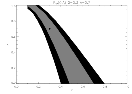
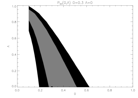
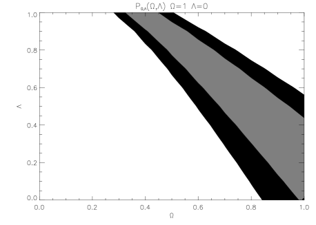
Fig. 4.: Contours of the $(\Omega,\Lambda)$ probability distribution obtained from a simulation on $1000$ clusters in the cases $(\Omega,\Lambda)=(0.3,0.7)$ (top panel) , $(\Omega,\Lambda)=(0.3,0)$ (middle panel) and $(1,0)$ (bottom panel). We give the $1\sigma=68\%$ (grey) and $2\sigma=95\%$ (dark) confidence levels.

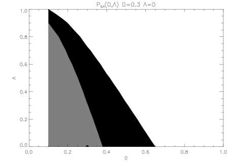
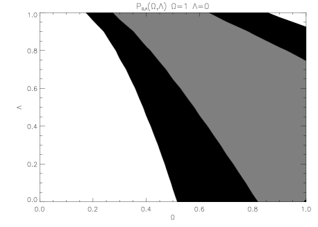
Fig. 5.: Contours of the $(\Omega,\Lambda)$ probability distribution obtained from a simulation on $100$ clusters in the cases $(\Omega,\Lambda)=(0.3,0.7)$ (top panel) , $(\Omega,\Lambda)=(0.3,0)$ (middle panel) and $(1,0)$ (bottom panel). We give the $1\sigma=68\%$ (grey) and $2\sigma=95\%$ (dark) confidence levels.

7 Conclusion

We have presented a method to constrain the cosmological parameters $(\Omega,\Lambda)$. It uses gravitational distortion produced by weak lensing around clusters and the photometric redshift of lensed galaxies. This purely geometrical method is insensitive to the lens modeling and can be directly applied to real data, that is the ellipticities of galaxies as observed from optical images. We have calculated the statistical noise coming mainly from the intrinsic source ellipticity and performed realistic simulations.
The main result is that with a short program of observations (about $20$ VLT nights) a constraint could be provided on the value of the cosmological constant. Using the observation of 100 clusters, we can reach $\Lambda_{-0.2}^{+0.3}$ in the case $\Omega+\Lambda=1$ or $\Omega_{-0.25}^{+0.3}$ in the case $\Lambda=0$ (at a $1\sigma$ level). These results could be even refined down to $10\%$ accuracy on $(\Omega,\Lambda)$ with the use of NGST. Indeed, the NGST looks perfectly suited for this method since it increases the number density of observed background galaxies.
We have estimated the amplitude of the systematics due to the presence of background structures with a multi-lensing model. It turns out that the shift amplitudes on the $(\Omega,\Lambda)$ determination are about $0.05$. One part of this systematic can be directly corrected. It concerns the perturbative effect due to galaxy-galaxy lensing (the correction of this effect need an approximate mean potential of galaxies and will be provided by the incoming galaxy-galaxy lensing investigations) . It also concerns the effect of background structures integrated along the line of sight (the correction of this effect requires calculations that takes in account the non linear evolution of large scale structures). It could be validated by ray tracing simulations.
In conclusion, we have shown that the systematic effects could be very well controlled by a judicious selection criteria of the clusters and the lensed galaxies of each triplet.
The $(\Omega,\Lambda)$ degeneracy of the triplet method is orthogonal to the one of the classical $(m,z)$ of supernovae searches. In this regards, when combined to the supernovae approach, the triplet method using VLT or NGST data could be extremely efficient. Therefore it seems important to investigate more deeply the possibility to use cluster lenses as practical tests to constrain the curvature of the Universe.

• We thank F. Bernardeau and L. van Waerbeke for fruitful discussions and their useful comments. This work was supported by the Programme National de Cosmologie.

Appendix A : The observed ellipticity of a background source

This appendix has two goals: firstly to recall the practical way to calculate the image ellipticity $\mbox{\boldmath$\epsilon$}_{I}=\epsilon_{I}e^{2i\theta_{I}}$ of a source from the image of a galaxy; secondly to express this ellipticity as a function of the potential of the lensing cluster through the local convergence $\kappa$ and complex shear $\mbox{\boldmath$\gamma$}=\gamma e^{2i\theta_{L}}$ (as it will be showed, the dependency in $\kappa,\gamma$ holds in the complex term $\mbox{\boldmath$g$}=\frac{\mbox{\boldmath$\gamma$}}{1-\kappa}$) and the intrinsic source ellipticity $\mbox{\boldmath$\epsilon$}_{S}=\epsilon_{S}e^{2i\theta_{S}}$.
For each background galaxy we can calculate a second order momentum matrix $M^{I}$, either directly from the image of the galaxy (see Bonnet 1995) either from the ACF of the single galaxy (see Van Waerbeke et al. 1997). Then the complex image ellipticity is derived from the momentum matrix through (see Seitz & Schneider 1997):

$$\mbox{\boldmath$\epsilon$}_{I}=\frac{M^{I}_{11}-M^{I}_{22}+2iM^{I}_{12}}{M^{I}_{11}+M^{I}_{22}+2\sqrt{det(M^{I})}}.$$ (84)

It is easy to check that this definition stays in agreement with equation (5). We also use a second order momentum matrix $M^{S}$ for the source as it would be seen with no lens.
The effect of the lens on the ellipticity of the background galaxy can then be summarized in the matrix equation (see Bonnet 1995):

$$M^{I} = \frac{AM^{S\ t}A}{|A|^{2}}\ \mbox{with}$$ (85)

$$A = \frac{(1-\kappa)I^{0}+\gamma J^{2\theta}}{(1-\kappa)^{2}-\gamma^{2}}.$$ (86)

In what follows and above, we use the notations

$$I^{2\theta}=\left(\begin{array}[]{lr}{\rm cos}(2\theta)&-{\rm sin}(2\theta)\\ {\rm sin}(2\theta)&{\rm cos}(2\theta)\end{array}\right),$$ (89)

$$J^{2\theta}=\left(\begin{array}[]{lr}{\rm cos}(2\theta)&{\rm sin}(2\theta)\\ {\rm sin}(2\theta)&-{\rm cos}(2\theta)\end{array}\right).$$ (92)

Equation (46) leads to

$$M^{I}=\frac{(I^{0}+gJ^{2\theta})I^{\theta}\left(\begin{array}[]{lr}\frac{1+\epsilon}{1-\epsilon}&0\\ 0&\frac{1-\epsilon}{1+\epsilon}\end{array}\right)I^{-\theta}(I^{0}+gJ^{2\theta})}{|1-g^{2}|}.$$ (95)

Using the following properties :

$$J^{\alpha}J^{\beta}=I^{\alpha-\beta},\ J^{\alpha}I^{\beta}=J^{\alpha-\beta},\ I^{\alpha}J^{\beta}=J^{\alpha+\beta},$$ (96)

equation (51) gives:

$$\begin{array}[]{ll}|1-g^{2}|(1-\epsilon_{S}^{2})\ M^{I}=&(1+\epsilon_{S}^{2})(1+g^{2})\\ &+4g\epsilon_{S}{\rm cos}(2(\theta_{S}-\theta_{L}))]I^{0}\\ &+2\epsilon_{S}J^{2\theta_{S}}+2g(1+\epsilon_{S}^{2})J^{2\theta_{L}}\\ &+2g^{2}\epsilon_{S}J^{4\theta_{L}-2\theta_{S}}.\end{array}$$

Finally, whatever the value of $g$ is (meaningly either in the weak or strong lensing regime) the measured image ellipticity writes:

$$\mbox{\boldmath$\epsilon$}_{I}=\frac{\mbox{\boldmath$\epsilon$}_{S}+(1+\epsilon_{S}^{2})\mbox{\boldmath$g$}+\mbox{\boldmath$\epsilon$}_{S}^{*}\mbox{\boldmath$g$}^{2}}{max(1,g^{2})+\epsilon_{S}^{2}min(1,g^{2})+\mbox{\boldmath$\epsilon$}_{S}^{*}\mbox{\boldmath$g$}+\mbox{\boldmath$\epsilon$}_{S}\mbox{\boldmath$g$}^{*}},$$ (97)

which, in the weak lensing and arclet regimes ($g<1$) simplifies into (to the third order in $\epsilon_{S}$ and $g$):

$$\mbox{\boldmath$\epsilon$}_{I}=(1-g^{2})\mbox{\boldmath$\epsilon$}_{S}+\mbox{\boldmath$g$}-\mbox{\boldmath$g$}^{*}\mbox{\boldmath$\epsilon$}_{S}^{2},$$ (98)

where the term $\mbox{\boldmath$g$}^{*}\mbox{\boldmath$\epsilon$}_{S}^{2}$ is negligible regarding to the term $\mbox{\boldmath$\epsilon$}_{S}$ and vanishes in $1/\sqrt{N}$ (because the argument of this term behaves randomly) in the operator G as the different noises described in section 3.4. Therefore the final equation for the image ellipticity writes :

$$\mbox{\boldmath$\epsilon$}_{I}=(1-g^{2})\mbox{\boldmath$\epsilon$}_{S}+\mbox{\boldmath$g$}.$$ (99)

It is worht noticing here that the term $(1-g^{2})$ is in favor of the method developed in this paper. Indeed, with the conditions used in the simulations (section 6), the mean value of this term is about $0.85$. It means that the noise coming from the intrinsic source ellipticity is lowered by $15\%$ or, for a given signal to noise ratio, the number of required clusters is lowered by $28\%$.

Appendix B : The case of a perturbing lens

This section will study the influence of a perturbative lens (galaxy, cluster or higher scale structure) located behind the principal lensing cluster on the measured ellipticity of a background source.
The calculation of the total amplification matrix in the case of two (or more) consecutive lenses has already been done (see for example Kovner 1997). The result can be simply noticed as follows:

$$A^{-1} = I^{0}-L-L^{P}+cL^{P}L\ \mbox{with}$$ (100)

$$L = \kappa I^{O}+\gamma J^{2\theta_{L}}\ \mbox{and}$$ (101)

$$L^{P} = \kappa^{P}I^{O}+\gamma^{P}J^{2\theta_{P}}.$$ (102)

The ^P upper index refers to the perturbative lens; $\kappa^{P}$ is defined as $\kappa$ in equation (3), just changing the principal lens noticed $l$ by the perturbative lens $l^{P}$ for the definition of the perturbative critical surface mass density $\Sigma_{crit}^{P}$. The $c$ coupling factor is $c=\frac{D_{LL^{P}}D_{OS}}{D_{OL^{P}}D_{LS}}$.
Equation (57) rewrites:

$$A^{-1}= (1-\kappa-\kappa^{P}+c\kappa\kappa^{P})I^{0}-\gamma(1-c\kappa^{P})J^{2\theta_{L}}$$

$$-\gamma^{P}(1-c\kappa)J^{2\theta_{P}}+c\gamma\gamma^{P}I^{2(\theta_{P}-\theta_{L})},$$

which can be inverted into

$$A=\frac{1}{|A^{-1}|} [(1-\kappa-\kappa^{P}+c\kappa\kappa^{P})I^{0}+\gamma(1-c\kappa^{P})J^{2\theta_{L}}$$

$$+\gamma^{P}(1-c\kappa)J^{2\theta_{P}}+c\gamma\gamma^{P}I^{2(\theta_{L}-\theta_{P})}].$$

Contrary to the case of a single lens where the Amplification matrix is symmetrical, here appears an anti-symmetric term, the last one of the above equation. However, even if the Amplification matrix is non symmetric, it keeps the propriety to transform an ellipse into another ellipse from the source plan to the image plan. Indeed the transformation from the source to the image can be represented by the vector notation $X_{S}=A^{-1}X_{I}$. To say that the source is an ellipse is equivalent to say that exists a matrix $E$ such that ${}^{t}X_{S}^{t}EEX_{S}=1$ (it comes from the fact that every positive symmetric matrix can be written as ${}^{t}EE$). So the position of image vectors writes ${}^{t}X_{I}^{t}\tilde{E}\tilde{E}X_{I}=1$ with $\tilde{E}=EA^{-1}$, which proves that the image is another ellipse. We thus can search for the image ellipticity of a source distorted by both lenses, as a function of the source ellipticity and the potential of the principal and perturbative lenses. We proceed the same way as in annex A.
In the following, we only keep second order terms in $\kappa,\kappa^{P},\gamma,\gamma^{P}\ and\ \epsilon_{S}$. So we can use the definitions:

$$\tilde{\mbox{\boldmath$g$}} = (1-\kappa-(1-c)\kappa^{P})^{-1}\mbox{\boldmath$\gamma$}$$ (105)

$$\tilde{\mbox{\boldmath$g$}}^{P} = (1-(1-c)\kappa-\kappa^{P})^{-1}\mbox{\boldmath$\gamma$}^{P}\ ,$$ (106)

and rewrite the amplification matrix:

$$A = \frac{I^{0}+\tilde{g}J^{2\theta_{L}}+\tilde{g}^{P}J^{2\theta_{P}}+c\tilde{g}\tilde{g}^{P}I^{2(\theta_{L}-\theta_{P})}}{1-\tilde{g}^{2}-\tilde{g}^{P2}-2(1-c)Re(\tilde{g}\tilde{g}^{P*})}.$$ (107)

Finally, with a calculation similar to the one done in annex A, we obtain for the image ellipticity:

$$\mbox{\boldmath$\epsilon$}_{I}= (1-|\tilde{\mbox{\boldmath$g$}}+\tilde{\mbox{\boldmath$g$}}^{P}|^{2})\mbox{\boldmath$\epsilon$}_{S}+\tilde{\mbox{\boldmath$g$}}+\tilde{\mbox{\boldmath$g$}}^{P}$$

$$-4cRe(\tilde{\mbox{\boldmath$g$}}\tilde{\mbox{\boldmath$g$}}^{P*}(\tilde{\mbox{\boldmath$g$}}+\tilde{\mbox{\boldmath$g$}}^{P})-2c\tilde{\mbox{\boldmath$g$}}^{*}\tilde{\mbox{\boldmath$g$}}^{P}\mbox{\boldmath$\epsilon$}_{S}-\epsilon_{S}^{2}(\tilde{\mbox{\boldmath$g$}}^{*}+\tilde{\mbox{\boldmath$g$}}^{P*})\,$$

which we simplify into

$$\mbox{\boldmath$\epsilon$}_{I}=(1-|\tilde{\mbox{\boldmath$g$}}+\tilde{\mbox{\boldmath$g$}}^{P}|^{2})\mbox{\boldmath$\epsilon$}_{S}+\tilde{\mbox{\boldmath$g$}}+\tilde{\mbox{\boldmath$g$}}^{P}.$$ (109)

In this last equation we have cancelled all the terms higher to the second order and oriented randomly (we consider that the source ellipticity, the principal and perturbative shears are independent. Terms higher to the second order with a random orientation give a negligible noise -regarding to the noise coming from the intrinsic source ellipticity- in the calculation of $G$).
Comparing equations (62) and (66) we can see the effect of the perturbative lens on the measured ellipticity:

1. Firstly a complex additive correction $\tilde{\mbox{\boldmath$g$}}^{P}$ which orientation is non correlated to the one of the cosmological term.

2. Secondly a scalar correction $(1-c)\kappa^{P}$ on the cosmological term $g$, due to coupling between the main and the perturbative lenses.
   

The simple form of equation (66) can be easily generalized to the case of a succession of many lenses noticed $L^{0}$ (instead of the principal lens), $L^{1}$ (instead of the perturbative lens), $L^{2}$, …, $L^{n}$ between the observer and the source noticed $S$. If the coupling factor between the lenses $i$ and $j$ (with $z_{i}<z^{j}$) is noticed $c_{i,j}^{S}=\frac{D_{OS}D_{L^{i}L^{j}}}{D_{OL_{j}}D_{L_{i}S}}$, then equation (55) giving the amplification matrix can be generalized into:

$$A^{-1}=\bigotimes_{i=n}^{i=0}(I^{0}-L^{i})=(I^{0}-L^{n})\otimes...\otimes(I^{0}-L^{0}),$$ (110)

where the $\otimes$ symbol defines a particular matrix product with the following properties: $I^{0}\otimes L^{i}=L^{i}\otimes I^{0}=L^{i}$, $L^{j}\otimes L^{i}=c_{i,j}^{S}L^{j}L^{i}$, $L^{k}\otimes L^{j}\otimes L^{i}=c_{i,j}^{S}c_{j,k}^{S}L^{k}L^{j}L^{i}$ etc…

We can remark that in the case of two very close lenses, their associated coupling factor $c$ is zero. With the same calculations and approximations as above we obtain:

$$\mbox{\boldmath$\epsilon$}_{I} = (1-|\sum_{i=0}^{i=n}\tilde{\mbox{\boldmath$g$}}^{i}|^{2})\mbox{\boldmath$\epsilon$}_{S}+\sum_{i=0}^{i=n}\tilde{\mbox{\boldmath$g$}}^{i}\ {\rm with}$$ (111)

$$\tilde{\mbox{\boldmath$g$}}^{i} = (1-\kappa^{i}-\sum_{j\neq i}(1-c_{i,j}^{S})\kappa^{j})^{-1}\gamma^{i}.$$ (112)