Systematic Construction of Exact MHD models for Astrophysical Winds and Jets

Abstract

By a systematic method we construct general classes of exact and selfconsistent axisymmetric MHD solutions describing flows which originate at the near environment of a central gravitating astrophysical object. The unifying scheme contains two large groups of exact MHD outflow models, (I) meridionally self-similar ones with spherical critical surfaces and (II) radially self-similar models with conical critical surfaces. The classification includes known polytropic models, such as the classical Parker model of a stellar wind and the Blandford and Payne (1982) model of a disk-wind; it also contains nonpolytropic models, such as those of winds/jets in Sauty and Tsinganos (1994), Lima et al (1996) and Trussoni et al (1997). Besides the unification of these known cases under a common scheme, several new classes emerge and some are briefly analysed; they could be explored for a further understanding of the physical properties of MHD outflows from various magnetized and rotating astrophysical objects in stellar or galactic systems.

1 Introduction

A widespread phenomenon is astrophysics is the outflow of plasma from the environment of stellar or galactic objects, either in the form of a noncollimated wind (Parker 1958, Feldman et al 1996), or, in the form of collimated jets (Blandford & Rees 1974, Biretta 1996, Ferrari et al, 1996). These outflows not only occur around typical stars and the nuclei of many radio galaxies and quasars, but they are also associated with young stars, older mass losing stars and planetary nebulae, symbiotic stars, black hole X-ray transients, low- and high-mass X-ray binaries and cataclysmic variables (for recent reviews see e.g., Ray 1996, Kafatos 1996, Mirabel & Rodriguez 1996, Livio 1997). Even for the two spectacular rings seen with the HST in SN1987A, it has been proposed that they may be inscribed by two precessing jets from an object similar to SS433 on a hourglass-shaped cavity which is created by nonuniform winds of the progenitor star (Burderi and King, 1995, Burrows et al 1995). Also recently, in the well known long jet of the distant radio galaxy NGC 6251 an about $10^{3}$ light-year-wide warped dust disk perpendicular to the main jet’s axis has been observed by HST to surround and reflect UV light from the bright core of the galaxy which probably hosts a black hole (Crane & Vernet 1997).

Nevertheless, despite their abundance the questions of the formation, acceleration and propagation of nonuniform winds and jets have not been fully resolved. One of the main difficulties in dealing with the theoretical problem posed by cosmical outflows is that their dynamics needs to be described - even to lowest order - by the highly intractable set of the MHD equations. As is well known, this is a nonlinear system of partial differential equations with several critical points, etc, and only very few classes of solutions are available for axisymmetric systems obtained by assuming a separation of variables in several key functions. This hypothesis allows an analysis in a 2-D geometry of the full MHD equations which reduce then to a system of ordinary differential equations. The basis of the self-similarity treatment is the prescription of a scaling law in the variables as a function of one of the coordinates. The choice of the scaling variable depends on the specific astrophysical problem.

In spherical coordinates ($r\,,\theta\,,\phi$), a first broad class for describing outflows are the so-called meridionally self-similar MHD models. Parker’s (1958) classical modeling of the spherically symmetric polytropic solar wind is the simplest member of this class. A new class of such type of models for describing magnetized and rotating MHD outflows from a central gravitating object has also been examined (Sauty & Tsinganos 1994 (henceforth ST94), Lima et al, 1996, Trussoni et al 1997). For example, an energetic criterion for the transition of an asymptotically conical outflow from an inefficient magnetic rotator to an asymptotically cylindrical outflow from an efficient magnetic rotator was derived. In the present paper, it will be shown that this special class of meridionally self-similar solutions is one of the simplest possible meridionally self-similar models. Furthermore, a new interesting member of this class of radially self-similar MHD models will be briefly sketched.

A second broad class of solutions contains the radially self-similar MHD models. Bardeen & Berger (1978) presented the first such models in the context of hydrodynamic and polytropic galactic winds. Nevertheless, their generalisation to a cold magnetized plasma by Blandford & Payne 1982 (henceforth BP82), remains widely known because of their success in showing for the first time that astrophysical jets can be accelerated magnetocentrifugally from a Keplerian accretion disk, if the poloidal fieldlines are inclined by an angle of 60^o, or less, to the disk midplane (but see also, Cao 1997). A further extension has been presented by Contopoulos & Lovelace (1994) for a hot plasma with a more general parametrization of the magnetic flux on the disc, while these models form the basis of several investigations of accretion-ejection flows from stars and AGN (Konigl 1989; Ferreira & Pelletier 1995; Ferreira 1997; Li 1995, 1996). In this paper it will be shown that this special class of radially self-similar solutions is one of the simplest possible such models. Furthermore, a new interesting member of the radially self-similar MHD models will be sketched.

In subsection 2.1 we use a simple theorem in order to construct several classes of meridionally selfsimilar solutions and the resulting cases are then summarized in Tables 1 and 2. The general method is next applied in subsection 2.2 to a step by step construction of a new model for collimated outflows which is also briefly sketched there. In section 3 the other remaining possibility in spherical coordinates, i.e., radial self similarity is taken up. The resulting cases are summarized in Table 3 while a new model is also briefly sketched which gives asymptotically cylindrical, paraboloidal and conical streamlines. Finally, the results are summarized in Sec. 4.

2 Meridionally selfsimilar
MHD outflows

Consider the steady ($\partial/\partial t=0$) hydromagnetic equations. They consist of a set of eight coupled, nonlinear, partial differential equations expressing momentum, magnetic and mass flux conservation, together with Faraday’s law of induction in the ideal MHD limit,

$$\rho\left(\vec{V}\cdot\vec{\nabla}\right)\vec{V}=\frac{\left(\vec{\nabla}\times\vec{B}\right)\times\vec{B}}{4\pi}-\vec{\nabla}P-\rho\vec{\nabla}{\cal V}\,,$$ (1)

$$\vec{\nabla}\cdot\vec{B}=0\,,\quad\vec{\nabla}\cdot\left(\rho\vec{V}\right)=0\,,\quad\vec{\nabla}\times\left(\vec{V}\times\vec{B}\right)=0\,.$$ (2)

$\vec{B}$, $\vec{V}$, $-\vec{\nabla}{\cal V}=-\vec{\nabla}\left(-{{\cal GM}}/{r}\right)$ denote the magnetic, velocity and external gravity fields, respectively, while $\rho$ and $P$ the gas density and pressure. With axisymmetry $(\partial/\partial\phi=0)$, we may introduce the magnetic flux function $A$, such that three free integrals exist for the total specific angular momentum carried by the flow and the magnetic field, $L(A)$, the corotation angular velocity of each streamline at the base of the flow, $\Omega(A)$ and the ratio of the mass and magnetic fluxes, $\Psi_{A}(A)$ (Tsinganos 1982). In terms of these integrals and the square of the poloidal Alvfén Mach number (or Alfvén number),

$$M^{2}=\frac{4\pi\rho V_{p}^{2}}{B_{p}^{2}}=\frac{\Psi_{A}^{2}}{4\pi\rho}\,,$$ (3)

the magnetic field and bulk flow speed are given in spherical coordinates $(r,\theta,\phi)$

$$\vec{B}=\vec{\nabla}\times\frac{A(r,\theta)\hat{\phi}}{r\sin\theta}-\frac{L\Psi_{A}-r^{2}\sin^{2}\theta\Omega\Psi_{A}}{r\sin\theta(1-M^{2})}\hat{\phi}\,,$$ (4)

$$\vec{V}=\frac{\Psi_{A}}{4\pi\rho}\vec{\nabla}\times\frac{A(r,\theta)\hat{\phi}}{r\sin\theta}+\frac{r^{2}\sin^{2}\theta\Omega-LM^{2}}{r\sin\theta(1-M^{2})}\hat{\phi}\,.$$ (5)

To construct classes of exact solutions, we shall make two crucial assumptions:

1. that the Alfvén number $M$ is some function of the dimensionless radial distance $R={r/r_{\star}}$,

   $$M=M(R)\,,$$ (6)

   and
   

2. that the poloidal velocity and magnetic fields have a dipolar angular dependence,

   $$A={r_{\star}^{2}B_{\star}\over 2}{\cal A}\left(\alpha\right)\,,\qquad\alpha=\frac{R^{2}}{G^{2}\left(R\right)}\sin^{2}\theta\,.$$ (7)

By choosing $G\left(R=1\right)=1$ at the Alfvén transition $R=1$, $G(R)$ evidently measures the cylindrical distance $\varpi$ to the polar axis of each fieldline labeled by $\alpha$, normalized to its cylindrical distance $\varpi_{\alpha}$ at the Alfvén point, $G\left(R\right)={\varpi}/{\varpi_{\alpha}}$. For a smooth crossing of the Alfvén sphere $R=1$ [$r=r_{\star},\theta=\theta_{a}(\alpha)$], the free integrals $L$ and $\Omega$ are related by

$${L\over\Omega}=\varpi_{\alpha}^{2}(A)=r_{\star}^{2}\sin^{2}\theta_{a}(\alpha)=r_{\star}^{2}\alpha\,.$$ (8)

Therefore, the second assumption is equivalent with the statement that at the Alfvén surface the cylindrical distance $\varpi_{\alpha}$ of each magnetic flux surface $\alpha=const$ is simply proportional to $\sqrt{\alpha}$.
Note also that the gravitational potential can be expressed in terms of the escape speed $V_{esc}$ at the Alfvén radius $r_{\star}$,

$${\cal V}=-\frac{\nu^{2}V_{\star}^{2}}{2R}\,,\qquad\nu=\frac{V_{esc}}{V_{\star}}\,,\qquad V_{esc}=\sqrt{\frac{2{\cal GM}}{r_{\star}}}\,.$$

Instead of using the three free functions of $\alpha$, (${\cal A}\,,\Psi_{A}$ , $\Omega$), we found it more convenient to work instead with the three dimensionless functions of $\alpha$, ($g_{1}$ , $g_{2}$ , $g_{3}$),

$$g_{1}\left(\alpha\right)=\int{\cal A}^{{}^{\prime}2}d\alpha\,,$$ (9)

$$g_{2}\left(\alpha\right)=\frac{r_{\star}^{2}}{B_{\star}^{2}}\int\Omega^{2}\Psi_{A}^{2}d\alpha$$ (10)

$$g_{3}\left(\alpha\right)=\frac{\Psi_{A}^{2}}{4\pi\rho_{\star}}\,.$$ (11)

Also, we shall indicate by ${\Pi}$ the total pressure in units of the magnetic pressure at the Alfvén surface on the polar axis, ${B_{\star}^{2}}/{8\pi}=\rho_{\star}V_{\star}^{2}/{2}$,

$$\Pi=\frac{8\pi}{B_{\star}^{2}}\left(P+\frac{B^{2}}{8\pi}\right)\,,$$

such that,

$$P=\frac{B_{\star}^{2}}{8\pi}\left({\Pi}+f_{1}g_{1}^{{}^{\prime}}+f_{2}\alpha g_{1}^{{}^{\prime}}+f_{3}\alpha g_{2}^{{}^{\prime}}\right)\,.$$ (12)

The functions $f_{i}(R)$, $i=1,2,3$ are given in Appendix A while all starred quantities refer to their respective values at the polar Alfvén point ($R=1$ ,$\alpha=0$). Hence,

$${\cal A}^{{}^{\prime}}\left(\alpha=0\right)=1\,,\;\Psi_{A}\left(\alpha=0\right)=\sqrt{4\pi\rho_{\star}}\,,$$

or,

$$g_{1}^{{}^{\prime}}\left(\alpha=0\right)=1\,,\;g_{3}\left(\alpha=0\right)=1\,.$$ (13)

With assumptions (i)-(ii) and in this notation, the $\hat{r}-$ and $\hat{\theta}-$ components of the momentum equation become,

$$\frac{\partial{\Pi}\left(R,\theta\right)}{\partial R}=f_{6}g_{1}^{{}^{\prime}}+\left(f_{7}+\frac{F}{R}f_{4}\right)\alpha g_{1}^{{}^{\prime}}+$$

$$\left(f_{8}+\frac{F}{R}f_{5}\right)\alpha g_{2}^{{}^{\prime}}+f_{9}g_{3}\,,$$ (14)

$$\frac{\partial{\Pi}\left(R,\theta\right)}{\partial\theta}=2\cot{\theta}\left(f_{4}\alpha g_{1}^{{}^{\prime}}+f_{5}\alpha g_{2}^{{}^{\prime}}\right)\,.$$ (15)

Next, by using $\alpha$ instead of $\theta$ as an independent variable, we may transform from pair of the independent variables ($R\,,\theta$) to pair of the independent variables ($R\,,\alpha$). With the following elementary relations valid for any differentiable function $\Phi$,

$$\frac{\partial{{\Phi}}\left(R,\theta\right)}{\partial R}=\frac{\partial{{\Phi}}\left(R,\alpha\right)}{\partial R}+\alpha\frac{F}{R}\frac{\partial{{\Phi}}\left(R,\alpha\right)}{\partial\alpha}\,,$$ (16)

$$\frac{\partial{{\Phi}}\left(R,\theta\right)}{\partial\theta}=2\alpha\cot\theta\frac{\partial{{\Phi}}\left(R,\alpha\right)}{\partial\alpha}\,,$$ (17)

we may transform Eqs. (2), (15) into the following two equations:

$$\frac{\partial{\Pi}\left(\alpha,R\right)}{\partial\alpha}=f_{4}g_{1}^{{}^{\prime}}+f_{5}g_{2}^{{}^{\prime}}\,,$$ (18)

$$\frac{\partial{\Pi}\left(\alpha,R\right)}{\partial R}=f_{6}g_{1}^{{}^{\prime}}+f_{7}\alpha g_{1}^{{}^{\prime}}+f_{8}\alpha g_{2}^{{}^{\prime}}+f_{9}g_{3}\,.$$ (19)

By integrating Eq. (18) we get ${\Pi}=f_{4}g_{1}+f_{5}g_{2}+f_{0}$ where $f_{0}$ is an arbitrary function of $R$. From Eq. (12) the pressure is

$$P=\frac{B_{\star}^{2}}{8\pi}\left(f_{4}g_{1}+f_{5}g_{2}+f_{0}+f_{1}g_{1}^{{}^{\prime}}+f_{2}\alpha g_{1}^{{}^{\prime}}+f_{3}\alpha g_{2}^{{}^{\prime}}\right)\,,$$ (20)

or,

$$P=\frac{B_{\star}^{2}}{8\pi}{\bf{Y}}{\bf{P}}^{{\dagger}}\,,$$

where P and Y are the (1 $\times$ 7) matrices,

$${\bf{P}}=\left[\;f_{0}\,\;f_{4}\,\;f_{1}\,\;f_{2}\,\;f_{5}\,\;f_{3}\,\;0\,\right]\,,$$ (21)

and

$$\begin{array}[]{l}{\bf{Y}}=\left[\;Y_{1}\,\;Y_{2}\,\;Y_{3}\,\;Y_{4}\,\;Y_{5}\,\;Y_{6}\,\;Y_{7}\;\right]=\\ \\ \left[\;1\;g_{1}\,\;g_{1}^{{}^{\prime}}\,\;\alpha g_{1}^{{}^{\prime}}\,\;g_{2}\,\;\alpha g_{2}^{{}^{\prime}}\,\;g_{3}\,\right]\,.\end{array}$$ (25)

Substituting for ${\Pi}$ in Eq. (19) it follows,

$$-f_{9}g_{3}-f_{8}\alpha g_{2}^{{}^{\prime}}+f_{5}^{{}^{\prime}}g_{2}-f_{7}\alpha g_{1}^{{}^{\prime}}-f_{6}g_{1}^{{}^{\prime}}+f_{4}^{{}^{\prime}}g_{1}+f_{0}^{{}^{\prime}}=0\,,$$ (26)

an expression of the form
$X_{7}\left(R\right)Y_{7}\left(\alpha\right)+X_{6}\left(R\right)Y_{6}\left(\alpha\right)+\cdots+X_{1}\left(R\right)Y_{1}\left(\alpha\right)=0\,,$

$$\mbox{or}\,,{\bf{Y}}{\bf{X}}^{{\dagger}}={\bf{0}}$$ (27)

with X the (1 $\times$ 7) matrix

$${\bf{X}}=\left[\;X_{1}\,\;X_{2}\,\;X_{3}\,\;X_{4}\,\;X_{5}\,\;X_{6}\,\;X_{7}\;\right]=$$

$$\left[\;f_{0}^{{}^{\prime}}\,\;f_{4}^{{}^{\prime}}\,\;-f_{6}\,\;-f_{7}\,\;f_{5}^{{}^{\prime}}\,\;-f_{8}\,\;-f_{9}\;\right]\,.$$ (28)

2.1 Systematic construction of classes of meridionally selfsimilar MHD outflows

Table 1: Meridionally Selfsimilar Models

Case	$g_{1}(\alpha)$	$g_{2}(\alpha)$	$g_{3}(\alpha)$	constants
(1)	$\alpha$	$\lambda^{2}\alpha$	$1+\delta\alpha$
(2)	$\alpha$	$\xi\alpha+{\mu\alpha^{\epsilon}/\epsilon}$	$1+\delta\alpha+\mu\delta_{0}\alpha^{\epsilon}$	$\epsilon\neq 0,1,\mu\neq 0$
(3)	$\alpha$	$\xi\alpha+\mu\alpha\ln{\alpha}$	$1+\delta\alpha+\mu\delta_{0}\alpha\ln{\alpha}$	$\mu\neq 0$
(4)	$\alpha_{0}e^{{\alpha\over\alpha_{0}}}$	$\lambda e^{{\alpha\over\alpha_{0}}}$	$1+\delta\alpha e^{{\alpha\over\alpha_{0}}}+\mu\left(e^{{\alpha\over\alpha_{0}}}-1\right)$
(5)	$\frac{\alpha_{0}}{\epsilon}\mid\frac{\alpha}{\alpha_{0}}-1\mid^{\epsilon-1}\left(\frac{\alpha}{\alpha_{0}}-1\right)$	$\xi\mid\frac{\alpha}{\alpha_{0}}-1\mid^{\epsilon}$	$1+\delta\mid\frac{\alpha}{\alpha_{0}}-1\mid^{\epsilon}+\mu\mid\frac{\alpha}{\alpha_{0}}-1\mid^{\epsilon-1}-\delta-\mu$	$\epsilon\neq 0,1$
(6)	$-\alpha_{0}\ln{\mid\frac{\alpha}{\alpha_{0}}-1\mid}$	$\xi\ln{\mid\frac{\alpha}{\alpha_{0}}-1\mid}$	$1+\delta\ln{\mid\frac{\alpha}{\alpha_{0}}-1\mid}+\mu\frac{\alpha}{\alpha_{0}\left(\alpha-\alpha_{0}\right)}$
(7)	$\frac{\alpha}{1-\alpha_{0}}$	$\mu\ln{\frac{\alpha}{\alpha_{0}}}+\xi\alpha$	$1+\delta\left(\alpha-\alpha_{0}\right)+\mu\delta_{0}\ln{\frac{\alpha}{\alpha_{0}}}$	$\mu\neq 0$
(8)	$\frac{\alpha_{0}}{\epsilon\left(1-\alpha_{0}\right)}\left(\frac{\alpha}{\alpha_{0}}\right)^{\epsilon}$	$\lambda_{1}\alpha^{\epsilon}+\lambda_{2}\alpha^{\epsilon-1}$	$1+\delta_{1}\left(\alpha^{\epsilon}-\alpha_{0}^{\epsilon}\right)+\delta_{2}\left(\alpha^{\epsilon-1}-\alpha_{0}^{\epsilon-1}\right)$	$\epsilon\neq 0,1$
(9)	$\frac{\alpha_{0}}{1-\alpha_{0}}\ln{\frac{\alpha}{\alpha_{0}}}$	$\lambda_{1}\ln{\frac{\alpha}{\alpha_{0}}}+{\lambda_{2}\over\alpha}$	$1+\delta_{1}\ln{\frac{\alpha}{\alpha_{0}}}+\delta_{2}\left(\frac{1}{\alpha}-\frac{1}{\alpha_{0}}\right)$

In (Vlahakis & Tsinganos 1997) the following simple theorem was proved:
Theorem: If $F_{n}(\alpha)$, $Y_{i}(\alpha)$, $X_{i}(R)$, $i=1,2,\cdots,n$ are arbitrary functions of the independent variables $\alpha$ and $R$ and

$$F_{n}\left(\alpha\right)=Y_{1}\left(\alpha\right)X_{1}\left(R\right)+\cdots+Y_{n}\left(\alpha\right)X_{n}\left(R\right),$$ (29)

then, there exist constants $c_{1},c_{2},\ldots,c_{n}$ such that,

$$F_{n}\left(\alpha\right)=c_{1}Y_{1}\left(\alpha\right)+c_{2}Y_{2}\left(\alpha\right)+\cdots+c_{n}Y_{n}\left(\alpha\right).$$ (30)

Consider then a relation of the form,

$$X_{n}\left(R\right)Y_{n}\left(\alpha\right)+\cdots+X_{1}\left(R\right)Y_{1}\left(\alpha\right)=0\,.$$ (31)

Regarding the first term of the sum there are evidently only two possibilities. Either,

1. $X_{n}\left(R\right)=0$ for every $R$, in which case (indicated by the digit ”0”) we have

   $$\qquad\quad X_{n-1}\left(R\right)Y_{n-1}\left(\alpha\right)+\cdots+X_{1}\left(R\right)Y_{1}\left(\alpha\right)=0\,,$$

   or,

2. $X_{n}\left(R\right)\neq 0$, in which case (indicated by the digit ”1”) we have

   $$\qquad\quad Y_{n}\left(\alpha\right)=-\frac{X_{1}\left(R\right)}{X_{n}\left(R\right)}Y_{1}\left(\alpha\right)-\cdots-\frac{X_{n-1}\left(R\right)}{X_{n}\left(R\right)}Y_{n-1}\left(\alpha\right)\,.$$

   • Then, according to the theorem stated in the beginning of this section, there are constants $\mu_{i}^{\left(n\right)},i=1,2,\cdots,n-1$ such that $Y_{n}\left(\alpha\right)=\sum_{i=1}^{n-1}\mu_{i}^{\left(n\right)}Y_{i}\left(\alpha\right)$. This gives a condition between the functions of $\alpha$. Substituting this in the initial sum we find:

   $$\begin{array}[]{l}\left[X_{n-1}\left(R\right)+\mu_{n-1}^{\left(n\right)}X_{n}\left(R\right)\right]Y_{n-1}\left(\alpha\right)+\\ \\ \left[X_{n-2}\left(R\right)+\mu_{n-2}^{\left(n\right)}X_{n}\left(R\right)\right]Y_{n-2}\left(\alpha\right)+\cdots\\ \\ +\left[X_{1}\left(R\right)+\mu_{1}^{\left(n\right)}X_{n}\left(R\right)\right]Y_{1}\left(\alpha\right)=0\,.\end{array}$$ (37)

Hence, in both cases we find a sum with $n-1$ terms. Following this algorithm at the end we ’ll have only one term. Since for each product we have the above two possibilities, totally we obtain $2^{n}$ cases. Each of them corresponds to a set ”xx$\cdots$xx” with $x=1,0\,$($n$ digits). The number of ”1” digits is the number of conditions between functions of $\alpha$ while the number of ”0” digits is the number of conditions between functions of $R$.

Now, following this method from Eq. (26) we get $2^{7}$ solutions. Each of them corresponds to a set ”xxxxxxx” with $x$ either 1, or, 0. Of those numbers:

1. The first digit is always ”1” (because $X_{7}\neq 0$).

2. The last digit is always ”0” (because $Y_{1}\neq 0$).

3. Since ${\cal A^{\prime}}\neq 0$, it follows that $g_{1}^{\prime}\neq 0$ and thus $g_{1}$ cannot be a constant. Hence, the function $Y_{2}=g_{1}$ cannot be proportional to $Y_{1}$ and therefore all numbers always have ”00” at the end.

4. We have totally six unknown functions: the three functions of $R$, ($G,M,f_{0}$) and the three functions of $\alpha$, ($g_{1},g_{2},g_{3}$). On the other hand, the number of conditions between the functions of $R$ (their number is equal to the number of digits ”0”) and the functions of $\alpha$ (their number equals to the number of digits ”1”) in each one of the sets ”xxxxxxx” is seven. It follows that the system of ($G,M,f_{0}$) and ($g_{1},\,g_{2},\,g_{3}$) is overdetermined. Note however that since the forms of the functions $X_{i}(R)$ are much more complicated than the forms of the functions $Y_{i}(\alpha)$, we choose sets ”xxxxxxx” with at most three ”0’s” because in the case of 4 or more ”0’s” we have correspondingly 4 or more relations between the 3 functions of $R$, which in general overdetermines the system of ($G,M,f_{0}$). We then shift the problem of overdetermination of the problem to the set of the 3 functions of $\alpha$, ($g_{1},\,g_{2},\,g_{3}$) which need to satisfy 4 relations. In this system however, it is possible to choose the constants $\mu_{i}^{\left(j\right)}$ such that a consistent solution for the functions of $\alpha$ can be finally constructed.

Altogether, then and with these considerations in mind, from the $2^{7}=128$ possible cases we end up with only five: 1011100, 1101100, 1110100, 1111000, 1111100. For each of one of those sets we can solve the system for $g_{1}\,,g_{2}\,,g_{3}$, as it is shown in the example of the next section.
From a different perspective, $g_{1}(\alpha),\,g_{2}(\alpha),\,g_{3}(\alpha)$ are vectors in a 3D $\alpha$-space with basis vectors [$u_{1}(\alpha)\,,u_{2}(\alpha)\,,u_{3}(\alpha)$]. This space contains all vectors $g_{i}(\alpha)$, $i=1,2,3$ subject to the $\theta$-selfsimilarity constraint manifested by Eq. (26), i.e., that for a given such set $g_{i}(\alpha)$, $i=1,2,3$, the vectors $1,\alpha g_{1}^{{}^{\prime}}(\alpha)\,,\alpha g_{2}^{{}^{\prime}}(\alpha)$ and $g_{1}^{{}^{\prime}}(\alpha)$ also belong to the same space. Each of the resulting functions $g_{i}(\alpha)$, $i=1,2,3$ are then a linear combination of the basis vectors $u_{1}(\alpha),u_{2}(\alpha),u_{3}(\alpha)$. In the following, we choose $u_{1}=1$, $u_{2}=g_{1}(\alpha)$. All such sets of basis vectors give all possible meridionally selfsimilar solutions. Therefore, collecting all possibilities, we end up with the classes of solutions shown in Table 1. Note that in the last three cases $A^{{}^{\prime}}\left(\alpha=0\right)\neq 1$, but one can say that the starred quantities refer to values at the point $R=1,\alpha=\alpha_{0}<1$.

In all nine cases of Table 1, from Eqs. (9), (10), (11) we may find easily the forms of the free integrals from the relations,

$$A=\frac{B_{\star}r_{\star}^{2}}{2}\int_{0}^{\alpha}\sqrt{g_{1}^{{}^{\prime}}}d\alpha,\;\;\Psi_{A}={\sqrt{4\pi\rho_{\star}g_{3}}}\,,$$

$${}\Omega=\frac{V_{\star}}{r_{\star}}\sqrt{\frac{g_{2}^{{}^{\prime}}}{g_{3}}}\,,\;\;L=r_{\star}V_{\star}\alpha\sqrt{\frac{g_{2}^{{}^{\prime}}}{g_{3}}}\,,$$ (38)

while by substituting $g_{1},g_{2},g_{3}$ in Eqs. (20), (26), the corresponding ordinary differential equations for the jet radius $G(R)$, Alfvén number $M(R)$ and pressure component $f_{0}(R)$ are found from the $R$-relations, as it is illustrated in the following section.
From the perspective of the $\alpha$-space, in each one of the cases of Table 1 there exists a $3\times 7$ matrix ${\bf{K}}$ such that

$${}{\bf{Y}}=\left[\;{u_{1}}\,\;{u_{2}}\,\;{u_{3}}\;\right]{\bf{K}}\,,$$ (39)

so that from Eq. (27),

$$\left[\;{u_{1}}\,\;{u_{2}}\,\;{u_{3}}\;\right]\,{\bf{K}}{\bf{X}}^{{\dagger}}={\bf{0}}\,.$$

If ${u_{i}}$ are linearly independent then

$${\bf{K}}{\bf{X}}^{{\dagger}}={\bf{0}}\,.$$

These three equations are the ordinary differential equations for the functions of $R$ in each model while the pressure is,

$$P=\frac{B_{\star}^{2}}{8\pi}\left[\;{u_{1}}\,\;{u_{2}}\,\;{u_{3}}\;\right]{\bf{K}}{\bf{P}}^{{\dagger}}=\frac{B_{\star}^{2}}{8\pi}\left(P_{0}+P_{1}g_{1}+P_{2}u_{3}\right)\,,$$

where

$${\bf K}{\bf P}^{{\dagger}}=[P_{0}\;P_{1}\;P_{2}]^{{\dagger}}\,.$$

The first two cases of Table 1 are of some interest. The first, is a degenerate one with $u_{3}=0$ and the following form of the free integrals:

$$\begin{array}[]{l}A=\frac{B_{\star}r_{\star}^{2}}{2}\alpha\,,\;\Psi_{A}=\sqrt{4\pi\rho_{\star}\left(1+\delta\alpha\right)}\,,\\ \\ \Omega=\frac{\lambda V_{\star}}{r_{\star}}\frac{1}{\sqrt{1+\delta\alpha}}\,.\end{array}$$ (43)

Table 2: Meridionally Selfsimilar Radial Models

Case	$g_{1}(\alpha)$	$g_{2}(\alpha)$	$g_{3}(\alpha)$
(1)	$-\ln{\mid 1-\alpha\mid}$	$0$	$1$
(2)	$\mu\int\frac{\alpha^{\epsilon}}{1-\alpha}d\alpha-\ln{\mid 1-\alpha\mid}$	$\lambda^{2}{\alpha^{\epsilon}\over\epsilon}$	$1+\delta\alpha^{\epsilon}$
(3)	$\mu_{1}\ln{\mid 1-\alpha\mid}+\mu_{2}\int\frac{\ln{\alpha}}{1-\alpha}d\alpha$	$\lambda\ln{\alpha}$	$\delta_{1}+\delta_{2}\ln{\alpha}$
(4)	$g_{1}(\alpha)\neq\mu_{1}\ln{\mid 1-\alpha\mid}+\mu_{2}$	$0$	$\delta g_{1}^{{}^{\prime}}\left(1-\alpha\right)+\lambda$
(5)	$\mu\ln{\mid 1-\alpha\mid}$	$g_{2}(\alpha)\neq(\mu,\mu_{1}\ln{\alpha}+\mu_{2},\mu_{1}\alpha^{\mu_{2}}+\mu_{3})$	$\delta$

This is a special case of the more general following case (2) for $\mu=0$ (and $\xi=\lambda^{2}$) and has been studied in detail in ST94 and Trussoni et al (1997). It is the single case where we have only two conditions between the functions of $R$, so that the third relation between the unknown functions $G,\,M,\,f_{0}$ is freely chosen. In Trussoni et al (1997) this corresponds to an a priori specification of the shape of the poloidal streamlines, while in ST94 in an a priori imposed relationship between the spherically and nonspherically symmetric components of the pressure. This last case leads to a generalized polytropic-type relation between pressure and density of the form,

$$\frac{P(\alpha,R)}{P(0,R)}=\mbox{ function of }\;\frac{\rho(\alpha,R)}{\rho(0,R)}\,.$$ (44)

As a result, a Bernoulli-type constant exists and, among others, this constant gives a quantitative criterion for the transition of an asymptotically conical wind from an inefficient magnetic rotator to an asymptotically cylindrical jet from an efficient magnetic rotator.
The second case with $\epsilon\neq 0,1,\mu\neq 0$ has $u_{2}=\alpha$, $u_{3}=\alpha^{\epsilon}$. The corresponding form of the free integrals is :

$$\begin{array}[]{l}A=\frac{B_{\star}r_{\star}^{2}}{2}\alpha,\;\Psi_{A}=\sqrt{4\pi\rho_{\star}\left(1+\delta\alpha+\mu\delta_{0}\alpha^{\epsilon}\right)}\,,\\ \\ \Omega=\frac{V_{\star}}{r_{\star}}\sqrt{\frac{\mu\alpha^{\epsilon-1}+\xi}{1+\delta\alpha+\mu\delta_{0}\alpha^{\epsilon}}}\,.\end{array}$$ (45)

This is a new case which emerged from the present systematic construction. The corresponding differential equations are derived in detail in the example of the next section where the solution is briefly analysed.
In the special configuration with $G=R\Leftrightarrow\alpha=\sin^{2}\theta$, the field and stream lines on the poloidal plane are radial and we find five cases shown in Table 2.
The first case is a degenerate one, wherein there is only one condition between the unknown functions $M(R)\,,f_{0}(R)$. Thus, a second relation between $M(R)-f_{0}(R)$ can be imposed a priori, for example, a polytropic relation between pressure and density. This last possibility leads precisely to Parker’s (1963) classical solar wind solution with a radial and nonrotating outflow. All other cases (2)-(5) are non-degenerate, i.e., there are two relations between $M(R)-f_{0}(R)$.
The second case has been analysed in detail in Lima et al (1996) and corresponds to a radial but heliolatitudinally depended outflow. In addition $\mu=-1$, $\epsilon=1$ this case coincides with (1) in Table 1 for radial poloidal streamlines. Note that a common feature of all rotating cases with radial stream lines on the poloidal plane is that they cannot be extended in all the poloidal plane, for sufficiently fast magnetic rotators. For example, in the model of Lima et al. (1996) the pressure becomes negative at some colatitude $\theta_{max}$, for large values of rotation. This is basically due to the fact that with the poloidal magnetic field dropping like $1/R^{2}$ and the azimuthal field dropping like $1/R$, the magnetic pressure drops like $1/R^{4}$ and by itself alone cannot balance the magnetic tension which drops like $1/R^{3}$; a strong pressure gradient is then needed from the pole towards the equator to balance the magnetic pinching. In fast magnetic rotators this pressure gradient is so strong that it leads to negative values of the pressure at angles $\theta>\theta_{max}$. A collimated outflow with uniform asymptotic conditions is the only way left for an everywhere valid outflow from an efficient magnetic rotator (Heyvaerts & Norman 1989, ST94).

2.2 Example of a new model for a meridionally self-similar MHD outflow

Let us illustrate the previous construction with the example 1101100 obtained from the present case with $n=7$. This number means the following:
Since the first digit is 1, there are six constants $\mu_{i}^{\left(7\right)},i=1,2,\cdots,6$ such that the following relation holds between the functions $Y_{i}(\alpha)$, i=1,2, ..7,

$$Y_{7}=\sum_{i=1}^{6}\mu_{i}^{\left(7\right)}Y_{i}\,,\qquad\mbox{($\alpha$-relation-1)}\,.$$ (46)

Substituting this expression of $Y_{7}$ in the initial relation Eq. (27) between the functions ($X_{i}$, $Y_{i}$), i=1,..7, we obtain

$$\begin{array}[]{l}\left(X_{6}+\mu_{6}^{\left(7\right)}X_{7}\right)Y_{6}+\left(X_{5}+\mu_{5}^{\left(7\right)}X_{7}\right)Y_{5}+\cdots+\\ \\ \left(X_{1}+\mu_{1}^{\left(7\right)}X_{7}\right)Y_{1}=0\,.\end{array}$$ (50)

Now the second digit is again 1 and thus there are five constants $\mu_{i}^{\left(6\right)},i=1,2,\cdots,5$ such that

$$Y_{6}=\sum_{i=1}^{5}\mu_{i}^{\left(6\right)}Y_{i}\,,\qquad\mbox{($\alpha$-relation-2)}\,,$$ (51)

while substituting this relation in Eq. (50) we obtain,

$$\begin{array}[]{l}\left[\left(X_{5}+\mu_{5}^{\left(7\right)}X_{7}\right)+\mu_{5}^{\left(6\right)}\left(X_{6}+\mu_{6}^{\left(7\right)}X_{7}\right)\right]Y_{5}+\cdots\\ \\ +\left[\left(X_{1}+\mu_{5}^{\left(7\right)}X_{7}\right)+\mu_{1}^{\left(6\right)}\left(X_{6}+\mu_{6}^{\left(7\right)}X_{7}\right)\right]Y_{1}=0\,.\end{array}$$ (55)

The third digit is 0 and hence

$$\begin{array}[]{l}\left(X_{5}+\mu_{5}^{\left(7\right)}X_{7}\right)+\mu_{5}^{\left(6\right)}\left(X_{6}+\mu_{6}^{\left(7\right)}X_{7}\right)=0\\ \\ \mbox{($R$-relation-1)}\end{array}$$ (59)

a relation between the functions of $R$. With the help of Eq. (59), Eq. (55) now reduces to,

$$\sum_{i=1}^{4}\left[\left(X_{i}+\mu_{i}^{\left(7\right)}X_{7}\right)+\mu_{i}^{\left(6\right)}\left(X_{6}+\mu_{6}^{\left(7\right)}X_{7}\right)\right]Y_{i}=0\,.$$ (60)

The fourth digit is 1 and thus there are three constants $\mu_{i}^{\left(4\right)},i=1,2,3$ such that

$$Y_{4}=\sum_{i=1}^{3}\mu_{i}^{\left(4\right)}Y_{i}\,,\qquad\mbox{($\alpha$-relation-3)}\,.$$ (61)

Substituting this relation in Eq. (60) we obtain

$$\begin{array}[]{l}\sum_{i=1}^{3}\left\{\left[\left(X_{i}+\mu_{i}^{\left(7\right)}X_{7}\right)+\mu_{i}^{\left(6\right)}\left(X_{6}+\mu_{6}^{\left(7\right)}X_{7}\right)\right]+\right.\\ \\ \left.\mu_{i}^{\left(4\right)}\left[\left(X_{4}+\mu_{4}^{\left(7\right)}X_{7}\right)+\mu_{4}^{\left(6\right)}\left(X_{6}+\mu_{6}^{\left(7\right)}X_{7}\right)\right]\right\}Y_{i}=0\,.\end{array}$$ (65)

The fifth digit is 1 and there are two constants $\mu_{i}^{\left(3\right)},i=1,2$ such that

$$Y_{3}=\mu_{1}^{\left(3\right)}Y_{1}+\mu_{2}^{\left(3\right)}Y_{2}\,,\qquad\mbox{($\alpha$-relation-4)}\,.$$ (66)

Substituting this in Eq. (65) we find a relation involving $Y_{1}$ and $Y_{2}$. Finally, we must put equal to zero the multipliers of $Y_{1},Y_{2}$ in this relation because the two remaining digits are 0. So we have

$$\begin{array}[]{l}\left[\left(X_{i}+\mu_{i}^{\left(7\right)}X_{7}\right)+\mu_{i}^{\left(6\right)}\left(X_{6}+\mu_{6}^{\left(7\right)}X_{7}\right)\right]+\\ \\ \mu_{i}^{\left(4\right)}\left[\left(X_{4}+\mu_{4}^{\left(7\right)}X_{7}\right)+\mu_{4}^{\left(6\right)}\left(X_{6}+\mu_{6}^{\left(7\right)}X_{7}\right)\right]+\\ \\ \mu_{i}^{\left(3\right)}\left(\left[\left(X_{3}+\mu_{3}^{\left(7\right)}X_{7}\right)+\mu_{3}^{\left(6\right)}\left(X_{6}+\mu_{6}^{\left(7\right)}X_{7}\right)\right]+\right.\\ \\ \left.\mu_{3}^{\left(4\right)}\left[\left(X_{4}+\mu_{4}^{\left(7\right)}X_{7}\right)+\mu_{4}^{\left(6\right)}\left(X_{6}+\mu_{6}^{\left(7\right)}X_{7}\right)\right]\right)=0\,,\\ \\ \mbox{ for }i=1,2\mbox{($R$-relations-2,3)}\,.\end{array}$$ (76)

These last two equations together with Eq. (59) are the three equations for the functions of $R$. On the other hand, Eq. (46), Eq. (51), Eq. (61) and Eq. (66) are four relations among the three functions of $\alpha$. These relations of the functions of $\alpha$ [Eqs. (66), (61), (51), (46)] are equivalent to the system:

$$\left.\begin{array}[]{llll}Y_{3}=c_{1}Y_{1}+c_{2}Y_{2}\\ Y_{4}=c_{3}Y_{1}+c_{4}Y_{2}\\ Y_{6}=c_{5}Y_{1}+c_{6}Y_{2}+c_{7}Y_{5}\\ Y_{7}=c_{8}Y_{1}+c_{9}Y_{2}+c_{10}Y_{5}\end{array}\right\}\Leftrightarrow\left\{\begin{array}[]{llll}g_{1}^{{}^{\prime}}=c_{1}+c_{2}g_{1}\\ \alpha g_{1}^{{}^{\prime}}=c_{3}+c_{4}g_{1}\\ \alpha g_{2}^{{}^{\prime}}=c_{5}+c_{6}g_{1}+c_{7}g_{2}\\ g_{3}=c_{8}+c_{9}g_{1}+c_{10}g_{2}\end{array}\right.$$ (85)

Note that we renamed the constants and also used Eq. (25). From the first, if $c_{2}\neq 0$ it follows that $g_{1}=-{c_{1}}/{c_{2}}+ce^{c_{2}\alpha}$. Then, from the second $c=0$ and hence $g_{1}=-{c_{1}}/{c_{2}}$. But $g_{1}$ cannot be a constant. Thus, $c_{2}=0$ while the first two equations combined with Eq. (13) give $g_{1}=\alpha+c_{11}$ while the third has the solutions:

$g_{2}=\left\{\begin{array}[]{lll}\frac{c_{6}}{1-c_{7}}\alpha+c_{12}+c_{13}\alpha^{c_{7}}\,,\;\mbox{if}\;\;c_{7}\neq 0,1\\ c_{6}\alpha\ln{\alpha}+c_{14}+c_{15}\alpha\,,\;\mbox{if}\;\;c_{7}=1\\ c_{6}\alpha+c_{16}\ln{\alpha}+c_{17}\,,\;\mbox{if}\;\;c_{7}=0\,.\end{array}\right.$

For the first possibility, we have finally the second case of Table 1 :

$\begin{array}[]{lll}g_{1}=\alpha\\ g_{2}=\xi\alpha+{\mu\alpha^{\epsilon}\over\epsilon}\;,\\ g_{3}=1+\delta\alpha+\mu\delta_{0}\alpha^{\epsilon}\end{array}\epsilon\neq 0,1$

where we have absorbed the constants $c_{11},c_{12}$ in the unknown function $f_{0}$, $c_{11}f_{4}+c_{12}f_{5}+f_{0}\rightarrow f_{0}$, Eqs. (20), (26).

After substituting these values of $g_{1},g_{2},g_{3}$ in Eqs. (20) - (26), we find that

$$\begin{array}[]{l}[f_{0}^{{}^{\prime}}-f_{6}-f_{9}]+\left[f_{4}^{{}^{\prime}}+\xi f_{5}^{{}^{\prime}}-f_{7}-\xi f_{8}-\delta f_{9}\right]\alpha+\\ \\ \mu\left[{f_{5}^{{}^{\prime}}}/{\epsilon}-f_{8}-\delta_{0}f_{9}\right]\alpha^{\epsilon}=0\,,\end{array}$$ (89)

and

$$\begin{array}[]{l}P=\frac{B_{\star}^{2}}{8\pi}\left(P_{0}+P_{1}\alpha+P_{2}\alpha^{\epsilon}\right)\\ \\ =\frac{B_{\star}^{2}}{8\pi}\left[f_{0}+f_{1}+\left(f_{4}+\xi f_{5}+f_{2}+\xi f_{3}\right)\alpha+\mu\left(\frac{f_{5}}{\epsilon}+f_{3}\right)\alpha^{\epsilon}\right]\,.\end{array}$$ (93)

By setting equal to zero the three expressions in the square brackets of Eq. (89) (since $\mu\neq 0$ and $1\,,\alpha\,,\alpha^{\epsilon}$ are linearly independent vectors in the $\alpha$-space for $\;\epsilon\neq 0,1\;$) we find the three R-relations for the functions $G(R)$, $M(R)$, $f_{0}(R)$ (which are the same with Eqs.(59),(76)). Using the functions $f_{4},F$ and the definitions of $P_{0}$ and $P_{1}$ we obtain five, first order, ordinary differential equations for $G(R)$, $F(R)$, $M(R)$ and the two pressure components $P_{1}(R)$ and $P_{0}(R)$,

$$\begin{array}[]{l}{dG^{2}\over dR}=-{{F-2}\over R}G^{2}\,,\end{array}$$ (94)

$$\begin{array}[]{l}\frac{dF}{dR}=\frac{F}{1-M^{2}}\frac{dM^{2}}{dR}-\frac{F\left(F-2\right)}{2R}-\\ \\ \frac{F^{2}-4}{2R\left(1-M^{2}\right)}-\frac{2G^{2}RP_{1}}{1-M^{2}}-\\ \\ \frac{2\xi R}{M^{2}\left(1-M^{2}\right)^{3}}\left[\left(2M^{2}-1\right)G^{4}-M^{4}+2M^{2}\left(1-G^{2}\right)\right]\end{array}$$ (100)

$$\begin{array}[]{l}\frac{dM^{2}}{dR}=\frac{M^{2}\left(1-M^{2}\right)}{\left(2M^{2}-1\right)G^{4}-M^{4}}\left\{-\epsilon\delta_{0}\nu^{2}\right.\frac{G^{2}\left(1-M^{2}\right)}{R^{2}}+\\ \\ \left.\frac{F-2}{R}\left[\left(\epsilon+1\right)M^{2}-\left(\epsilon-1\right)G^{4}\right]\right\}\end{array}$$ (104)

$$\begin{array}[]{l}\frac{dP_{1}}{dR}=-\left[\frac{F^{2}-4}{2R^{2}G^{2}}+2\xi\frac{\left(1-G^{2}\right)^{2}}{G^{2}\left(1-M^{2}\right)^{3}}\right]\frac{dM^{2}}{dR}-\\ \\ \frac{M^{2}F}{2R^{2}G^{2}}\frac{dF}{dR}-\frac{\delta\nu^{2}}{R^{2}M^{2}}-\frac{M^{2}\left(F^{2}-4\right)\left(F-4\right)}{4R^{3}G^{2}}+\\ \\ \xi\frac{\left(F-2\right)\left[\left(2M^{2}-1\right)G^{4}-M^{4}\right]}{RG^{2}M^{2}\left(1-M^{2}\right)^{2}}\end{array}$$ (110)

$$\begin{array}[]{l}\frac{dP_{0}}{dR}=-\frac{2}{G^{4}}\frac{dM^{2}}{dR}-\frac{\nu^{2}}{R^{2}M^{2}}-\frac{2M^{2}\left(F-2\right)}{RG^{4}}\end{array}$$ (112)

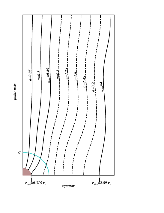
Figure 1: Poloidal field and streamlines close to the stellar base for the asymptotically cylindrical $\theta$-self similar model of case (2) from Table 1, for the following set of parameters: $\epsilon=0.5$, $\nu^{2}=2{\cal GM}/r_{\star}V_{\star}^{2}=10$, $\delta\nu^{2}=3.5$, $\delta_{0}\nu^{2}=0.1$, $\xi=-10$, $\mu=20$, $p_{\star}=\left({dM^{2}}/{dR}\right)_{\star}=1.6$,$F_{\star}=1.1$.

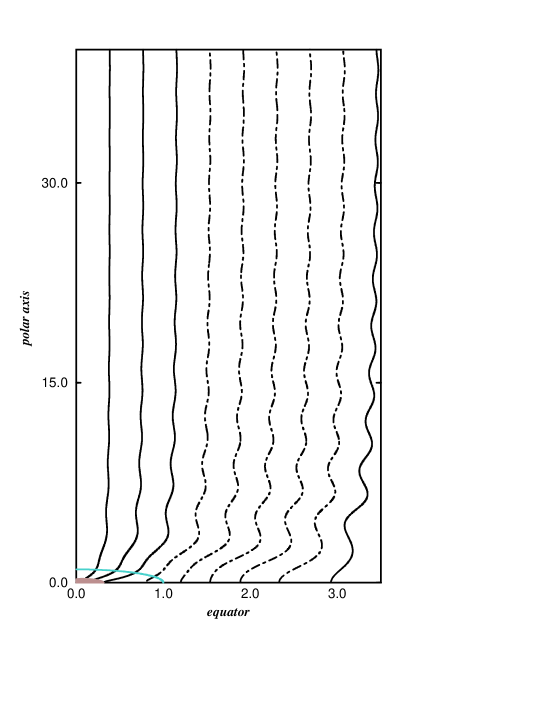
Figure 2: Poloidal field and streamlines as in Fig (1), but in an enlarged scale to show the asymptotical collimation reached after the oscillations have decayed.

Note that the third pressure component $P_{2}(R)$ is given explicitly in terms of $M$ and $G$ ($f_{3}$ and $f_{5}$). An integration of the above set of equations will give the complete solution. However, this exercise is rather complicated since any physically accepted solution should pass through the various MHD critical points (Tsinganos et al 1996). This undertaking, together with a discussion of the solution and application to collimated outflows is the subject of the next paper.

It is worth mentioning at this point that our analysis of model (2) of Table 1 shows that mainly cylindrically collimated solutions are obtained. The set of Figures (1-2) illustrates such a typical solution for a representative set of the constants describing the particular model. This solution crosses the Alfvén surface for appropriate values of the slope of the square of the Alfvén number $p_{\star}=\left({dM^{2}}/{dR}\right)_{\star}$, the expansion function $F_{\star}$ and $P_{1\star}$ which satisfy the Alfvén regularity condition (Heyvaerts & Norman 1989, ST94) which is easily obtained from Eq. (143) of Appendix A at ($R=G=M=1$), i.e.,

$$F_{\star}p_{\star}=2f_{4\star}\,.$$ (113)

The nonspherically symmetric part of the pressure $P_{1\star}$ is obtained from its definition while the functions $f_{3\star}\,,f_{5\star}$ are calculated for $R=1$ using the L’Hospital rule. Figs. (1,2,3) correspond to the set $F_{\star}=1.1$ and $p_{\star}=1.6$. Note that after the Alfvén star-type critical point is crossed, the modified by self-similarity X-type fast critical point (Tsinganos et al 1996) may be crossed by further adjusting appropriately the triplet of the variables $(F_{\star}\,,p_{\star}\,,P_{1\star})$. It suffices to note that solutions crossing only the Alfvén surface do not differ qualitatively from those which in addition cross the modified by the present meridional selfsimilarity fast critical surface.

Fig. (1) shows the shape of the streamlines on the poloidal plane and close to the Alfvén surface. The cylindrical asymptotical shape of the poloidal streamlines is shown in the enlarged scale of Fig (2). Note also the constant wavelength but the decaying with distance amplitude of the oscillations, in full agreement with the analysis in Vlahakis & Tsinganos (1997). At the last shown fieldline $\alpha_{out}=4$, the toroidal fields vanish $B_{\phi}=0$, $V_{\phi}=0$.For $\alpha>\alpha_{out}\,,\Omega^{2}$ becomes negative , so there is no solution there. The same oscillatory behaviour can be seen in the fieldlines which are not rooted on the star but they are perpendicular to a thin disk around it (dotted curves in Figs 1, 2.)

Figure 3: Outflow velocities in units of $V_{\star}$, the radial speed at the Alfvén point $(\alpha=0,R=1)$, for the parameters given in the caption of Fig. (1) of model (2) of Table 1.

The oscillatory structure of all flow speeds before the flow reaches full cylindrical collimation is also shown in Fig. (3) where we have plotted the characteristic velocities in units of the Alfvén speed at the polar axis and Alfvén sphere ($\alpha=0\,,R=1$), $V_{\star}$.

The poloidal speed along the polar axis $V_{p,pol}$ increases to a uniform superAlfvénic value and is higher than the same speed along the limiting streamline $V_{p,lim}$ (i.e., the last fieldline rooted on the stellar base $r_{star}$ taken to be at $0.315r_{\star}$). Both reach asymptotically uniform values after $V_{p,lim}$ intersects the curve of the poloidal Alfvén speed $V_{Ap,lim}$ at $R=1$. Note that corotation may be seen up to the Alfvén distance $R=1$: the azimuthal speed $V_{\phi,lim}$ at the ’limiting fieldine’ increases until the Alfvén surface is reached and drops from angular momentum conservation as the outflow expands almost conically. Further away however, this speed too levels off to a constant value when full collimation is achieved, as expected. Finally, the fact that the jet has a large component of toroidal field is reflected by the large values of the Alfvén speed associatd with the toroidal magnetic field, $V_{A\phi,lim}$, as compared to the rotational speed $V_{\phi,lim}$.

3 Systematic construction of classes of radially selfsimilar MHD outflows

To construct general classes of radially self-similar solutions, we make the following two key assumptions:
(i) the Alfvén Mach number $M$ is solely a function of $\theta$,

$$M=M(\theta)\,,\qquad M(\theta_{\star})=1\,,$$ (114)

and
(ii) that the poloidal velocity and magnetic fields have a dipolar angular dependence,

$$A=\frac{B_{o}\varpi_{o}^{2}}{2}{\cal A}\left(\alpha\right)\,,\qquad\alpha=\frac{R^{2}}{G^{2}\left(\theta\right)}\sin^{2}\theta\,,\quad R={r\over\varpi_{o}}\,,$$ (115)

where $B_{o},\varpi_{o}$ are constants. By choosing $G\left(\theta_{\star}\right)=1$ at the Alfvén transition $\theta_{\star}$, $G(\theta)$ evidently measures the cylindrical distance $\varpi$ to the polar axis of each fieldline labeled by $\alpha$, normalized to its cylindrical distance $\varpi_{\alpha}$ at the Alfvén point, $G\left(\theta\right)={\varpi}/{\varpi_{\alpha}}$. For a smooth crossing of the Alfvén cone $\theta=\theta_{\star}$ [$r=r_{\alpha}\left(\alpha\right),\theta=\theta_{\star}$], the free integrals $L$ and $\Omega$ are related by

$${L\over\Omega}=\varpi_{\alpha}^{2}(A)=r_{\alpha}^{2}\left(\alpha\right)\sin^{2}\theta_{\star}=\varpi_{o}^{2}\alpha\,.$$ (116)

Therefore, the second assumption is equivalent with the statement that at the Alfvén conical surface, the cylindrical distance $\varpi_{a}$ of each magnetic flux surface $\alpha=const$ is simply proportional to $\sqrt{\alpha}$, exactly as in the previous meridionally self-similar case.
Instead of using the three functions of $\alpha$, (${\cal A}\,,\Psi_{A}$, $\Omega$) we found it more convenient to work with the three dimensionless functions of $\alpha$, ($q_{1}\,,q_{2}\,,q_{3}$),

$$q_{1}\left(\alpha\right)=\int{{\cal A}^{{}^{\prime}2}\over\alpha}d\alpha\,,$$ (117)

$$q_{2}\left(\alpha\right)=\frac{\varpi_{o}^{2}}{B_{o}^{2}}\int\Omega^{2}\Psi_{A}^{2}d\alpha\,,$$ (118)

$$q_{3}\left(\alpha\right)=\frac{{\cal GM}}{B_{o}^{2}\varpi_{o}}\int\frac{\Psi_{A}^{2}}{\alpha^{{3\over 2}}}d\alpha\,.$$ (119)

Following the same algorithm as in the previous case, we shall use ($\alpha\,,\theta$) as the independent variables and transform the derivatives with respect to $r$ and $\theta$ to derivatives with respect to $\alpha$ and $\theta$ in the $\hat{r}$- and $\hat{\theta}$-components of the momentum equation. Integrating the resulting $\hat{r}$–component of the momentum equation we get

$$P=\frac{B_{o}^{2}}{8\pi}\left(h_{1}\alpha q_{1}^{{}^{\prime}}+h_{2}\alpha q_{2}^{{}^{\prime}}+h_{3}q_{2}+h_{4}q_{3}+h_{5}q_{1}+h_{0}\right)\,,$$ (120)

or

$$P=\frac{B_{o}^{2}}{8\pi}\bf{Y}\bf{P}^{{\dagger}}$$

with

$${\bf{P}}=\left[\;h_{0}\;h_{5}\;h_{1}\;h_{3}\;h_{2}\;h_{4}\;0\;\right]\,,$$ (121)

and

$$\begin{array}[]{l}{\bf{Y}}=\left[\;Y_{1}\;Y_{2}\;Y_{3}\;Y_{4}\;Y_{5}\;Y_{6}\;Y_{7}\;\right]=\\ \\ \left[\;1\;q_{1}\;\alpha q_{1}^{{}^{\prime}}\;q_{2}\;\alpha q_{2}^{{}^{\prime}}\;q_{3}\;\alpha q_{3}^{{}^{\prime}}\;\right]\,,\end{array}$$ (125)

and after substituting the pressure in the other component of the momentum equation we obtain

$$\begin{array}[]{l}Hh_{4}\alpha q_{3}^{{}^{\prime}}+h_{4}^{{}^{\prime}}q_{3}+h_{3}\left(H-2\right)\alpha q_{2}^{{}^{\prime}}+h_{3}^{{}^{\prime}}q_{2}+\\ \\ \frac{\left(h_{1}\left[1-M^{2}\right]^{2}\right)^{{}^{\prime}}\alpha q_{1}^{{}^{\prime}}}{\left(1-M^{2}\right)}+h_{5}^{{}^{\prime}}q_{1}+h_{0}^{{}^{\prime}}=0\,,\end{array}$$ (129)

where a prime in the functions of $q_{i}(\alpha)$, i=1,2,3 and $h_{i}$ indicates a derivative with respect to their variables $\alpha$ and $\ln\sin\theta$, respectively, while the functions $h_{j}\left(\theta\right),j=1,2,3,4,5$ and $H$ are given in Appendix B.
This expression is again of the form
$X_{7}\left(\theta\right)Y_{7}\left(\alpha\right)+X_{6}\left(\theta\right)Y_{6}\left(\alpha\right)+\cdots+X_{1}\left(\theta\right)Y_{1}\left(\alpha\right)=0\,,$

$$\mbox{or}\,,{\bf{Y}\bf{X}}^{{\dagger}}={\bf{0}}$$ (130)

with X the (1 $\times$ 7) matrix

$$\begin{array}[]{l}{\bf{X}}=\left[\;X_{1}\;X_{2}\;X_{3}\;X_{4}\;X_{5}\;X_{6}\;X_{7}\;\right]=\\ \\ \left[h_{0}^{{}^{\prime}}\;h_{5}^{{}^{\prime}}\;\frac{\left(h_{1}\left[1-M^{2}\right]^{2}\right)^{{}^{\prime}}}{\left(1-M^{2}\right)}\;h_{3}^{{}^{\prime}}\;h_{3}\left(H-2\right)\;h_{4}^{{}^{\prime}}\;Hh_{4}\;\right]\,.\end{array}$$ (134)

As in the previous case of meridionally selfsimilar solutions, we classify the various possibilities by the sets $xxxxxxx$. And, these sets always have ”00” at the end, their first digit is ”1”, they have at most three ”0’s”, while from the $2^{7}$ possibilities we end up again with the cases 1011100, 1101100, 1110100, 1111000, 1111100. Now the vectors $q_{1}(\alpha),\,q_{2}(\alpha),\,q_{3}(\alpha)$ belong to a 3D $\alpha$-space with basis vectors [$e_{1}(\alpha)\,,e_{2}(\alpha)\,,e_{3}(\alpha)$]. This space contains all vectors $q_{i}(\alpha)$, $i=1,2,3$ subject to the $r$-selfsimilarity constraint manifested by Eq. (129), i.e., that for a given such set $q_{i}(\alpha)$, $i=1,2,3$, the vectors $1,\alpha q_{i}^{{}^{\prime}}(\alpha)$ , $i=1,2,3$ also belong to the same space. Each of the functions $q_{i}(\alpha)$, $i=1,2,3$ which satisfy this constraint are then a linear combination of the basis vectors $e_{1}(\alpha),e_{2}(\alpha),e_{3}(\alpha)$. In the following, we choose $e_{1}=1$, $e_{2}=q_{1}(\alpha)$. All such sets of basis vectors give all possible radially selfsimilar solutions. Therefore, collecting all possibilities, we end up with the 6 classes of solutions shown in Table 3.

Table 3: Radially Selfsimilar Models

Case	$q_{1}(\alpha)$	$q_{2}(\alpha)$	$q_{3}(\alpha)$	constants
(1)	$\frac{E_{1}}{F-2}\alpha^{F-2}$	$\frac{D_{1}}{F-2}\alpha^{F-2}$	$\frac{C_{1}}{F-2}\alpha^{F-2}$	$E_{1},F-2\neq 0$
(2)	$E_{1}\ln{\alpha}$	$D_{1}\ln{\alpha}$	$C_{1}\ln{\alpha}$	$E_{1}\neq 0$
(3)	$E_{1}\alpha^{x_{1}}+E_{2}\alpha^{x_{2}}$	$D_{1}\alpha^{x_{1}}+D_{2}\alpha^{x_{2}}$	$C_{1}\alpha^{x_{1}}+C_{2}\alpha^{x_{2}}$	$E_{1}^{2}+D_{1}^{2}+C_{1}^{2},E_{2},x_{1},x_{2},x_{1}-x_{2}\neq 0$
(4)	$E_{1}\ln{\alpha}+E_{2}\alpha^{x}$	$D_{1}\ln{\alpha}+D_{2}\alpha^{x}$	$C_{1}\ln{\alpha}+C_{2}\alpha^{x}$	$E_{i}^{2}+D_{i}^{2}+C_{i}^{2},x\neq 0,i=1,2$
(5)	$E_{1}\left(\ln{\alpha}\right)^{2}+E_{2}\ln{\alpha}$	$D_{1}\left(\ln{\alpha}\right)^{2}+D_{2}\ln{\alpha}$	$C_{1}\left(\ln{\alpha}\right)^{2}+C_{2}\ln{\alpha}$	$E_{1}^{2}+D_{1}^{2}+C_{1}^{2}\neq 0$
(6)	$E_{1}\alpha^{x}\ln{\alpha}+E_{2}\alpha^{x}$	$D_{1}\alpha^{x}\ln{\alpha}+D_{2}\alpha^{x}$	$C_{1}\alpha^{x}\ln{\alpha}+C_{2}\alpha^{x}$	$E_{1}^{2}+D_{1}^{2}+C_{1}^{2}\neq 0$

In all of the cases of Table 3, from Eqs. (117), (118), (119) we find the form of the functions of $\alpha$,

$$A=\frac{B_{o}\varpi_{o}^{2}}{2}\int_{0}^{\alpha}\sqrt{\alpha q_{1}^{{}^{\prime}}}d\alpha\,,\qquad\Psi_{A}^{2}=\frac{B_{o}^{2}\varpi_{o}}{{\cal GM}}\alpha^{{3\over 2}}q_{3}^{{}^{\prime}}\,,$$

$$\Omega^{2}=\frac{{\cal GM}}{\varpi_{o}^{3}}\frac{q_{2}^{{}^{\prime}}}{q_{3}^{{}^{\prime}}}\alpha^{-{3\over 2}}\,,\qquad L^{2}={\cal GM}\varpi_{o}\frac{q_{2}^{{}^{\prime}}}{q_{3}^{{}^{\prime}}}\alpha^{{1\over 2}}\,.$$ (135)

Finally, by substituting $q_{1}\,,q_{2}\,,q_{3}$ in Eqs. (120) , (129), we find the ordinary differential equations which the functions $G(\theta)\,,M(\theta)\,,h_{0}(\theta)$ obey.
In $\alpha$-space, for each of the cases of Table 3 there exists a (3 $\times$ 7) matrix ${\bf{K}}$ such that

$${}{\bf{Y}}=\left[\;{e_{1}}\,\;{e_{2}}\,\;{e_{3}}\;\right]\;\;{\bf{K}}\,,$$ (136)

and from Eq. (130)

$$\left[\;{e_{1}}\,\;{e_{2}}\,\;{e_{3}}\,\right]\;{\bf{K}}{\bf{X}}^{{\dagger}}={\bf{0}}\,.$$

If the basis vectors ${e_{i}}$ are linearly independent, then,

$${\bf{K}}{\bf{X}}^{{\dagger}}={\bf{0}}\,.$$

These three equations are the ordinary differential equations for the functions of $\theta$ in each model of Table 3, while for the pressure,

$$P=\frac{B_{o}^{2}}{8\pi}\left[\;{e_{1}}\,\;{e_{2}}\,\;{e_{3}}\,\right]{\bf{K}}{\bf{P}}^{{\dagger}}=\frac{B_{\star}^{2}}{8\pi}\left(P_{0}+P_{1}q_{1}+P_{2}e_{3}\right)\,,$$

where

$${\bf K}{\bf P}^{{\dagger}}=[P_{0}\;P_{1}\;P_{2}]^{{\dagger}}\,.$$

As with the previous meridionally selfsimilar solutions, the first two classes are of particular interest. The first corresponds to the following form of the free integrals:

$$A=\frac{B_{o}\varpi_{o}^{2}\sqrt{E_{1}}}{F}\alpha^{{F\over 2}}\,,\;\Psi_{A}^{2}=\frac{C_{1}B_{o}^{2}\varpi_{o}}{{\cal GM}}\alpha^{(F-3/2)}\,,$$

$$\Omega^{2}=\frac{D_{1}{\cal GM}}{\varpi_{o}^{3}C_{1}}\alpha^{-{3\over 2}}\,.$$ (137)

This is a degenerate case, i.e., $e_{3}=0$ and we have only two conditions between the functions of $\theta$. It follows that we are free to impose a third relation between the unknown functions $[G(\theta)\,,M(\theta)\,,h_{0}(\theta)]$. One possibility is that such a third imposed relation is of the polytropic type, $P\propto\rho^{\gamma}$ (in this case $h_{0}=0$). In such a polytropic case which has been analysed in detail in Contopoulos & Lovelace (1995), the magnetic flux is of the form $A=f_{f}(\theta)R^{F}$ with $f_{f}(\theta)\propto[\sin\theta/G(\theta)]^{F}$ (for notation see also Tsinganos et al 1996). The magnetic field at the equatorial plane $\theta=90^{o}$ is $B\propto R^{F-2}$, the density $\rho\propto R^{2F-3}$, while the sound, Alfvén and rotational speeds scale as their Keplerian counterparts, i.e., as $R^{-1/2}$. Note that if $[{D_{1}G\left({\pi}/{2}\right)}/{C_{1}}]\left[{(G^{2}-M^{2})}/{G\left(1-M^{2}\right)}\right]_{\theta=\frac{\pi}{2}}^{2}=1$, the rotational velocity at the equatorial plane is exactly Keplerian. The classical and simplest subcase analysed in BP82 corresponds to the subclass with $F=3/4$, wherein $B\propto R^{-5/4}$. The two relations among the functions of $\theta$ are the two resulting first order differential equations for the Alfvén number $M(\theta)$ and dimensionless radius $G(\theta)$ [$m(\chi)=M^{2}(\theta)$ and $\xi(\chi)={G(\theta)}/{G(\frac{\pi}{2})}$ in the notation of BP82].
The second case is also degenerate since $e_{3}=0$ with again only two conditions between the functions of $\theta$. As before, we are free to impose a third relation between the unknown functions $[G(\theta)\,,M(\theta)\,,h_{0}(\theta)]$, for example, a polytropic relationship. Then one can prove that this case is a subcase of the first one (if it is polytropic), for $F=2$. All other cases shown in Table 3 are nondegenerate.

The third class, is characterized first by a set of parameters describing the particular model and the dependance of the free integrals on the magnetic flux function $A\left(\alpha\right)$, ($x_{1}\,,x_{2}\,,E_{1}\,,E_{2}\,,C_{1}\,,C_{2}\,,D_{1}\,,D_{2})$. Second by the Alfvén angle $\theta_{\star}$. And third, by the set of the critical point parameters $p_{\star}=\left({dM^{2}}/{d\theta}\right)_{\star}$ and $\varphi_{\star}$ which denote the slope of the Alfvén number and the expansion angle, respectively, at the Alfvén angle $\theta_{\star}$, together with the pressure component $P_{1\star}$ through $h_{5\star}$. This triplet of ’dynamical’ parameters fixes the physical solution and they are related through the Alfvén regularity condition which is now obtained from Eq. (B) of Appendix B at the Alfvén angle $\theta_{\star}$ where $M=G=1$ and $h_{5}=h_{5\star}$, i.e.,  .

$$h_{5\star}=-{\sin^{2}\theta_{\star}\tan(\theta_{\star}+\varphi_{\star})}p_{\star}\,.$$ (138)

As with the previous case of meridional selfsimilarity, this condition relates the slope of the square of the Alfvén number $p_{\star}=\left({dM^{2}}/{d\theta}\right)_{\star}$ and the expansion angle $\varphi_{\star}$ with the pressure component $P_{1\star}$ through $h_{5\star}$. Finally, the requirement that the solution crosses the two slow and fast X-type critical points (modified by the radial self-similarity assumption, Tsinganos et al 1996) determines all these three ’dynamical’ parameters $[\varphi_{\star}\,,p_{\star}\,,P_{1\star}]$.

It is interesting to note that contrary to classes (1)-(2) in Table 3, this model (3) may be characterized by a scale, for example the radial distance on the plane of the disk where the magnitudes of the poloidal speed and magnetic field or the toroidal speed and magnetic field become zero. Hence, it occured to us that this is an interesting generalisation of the BP82 model and therefore worthy of further investigation.

Figure 4: Field and streamlines for the cylindrical $r$-self similar model of case (3) from Table 3 and the following set of parameters: $x_{1}=-0.6$, $x_{2}=-0.5$, $E_{1}=-0.03$, $E_{2}=0.03$, $C_{1}=-1.5$, $C_{2}=-0.6$, $D_{1}=-25$, $D_{2}=-10$, $\theta_{\star}=62^{o}$, $\varphi_{\star}=55^{o}$, $p_{\star}=-3$. At the disk level, $V_{\phi}\propto R^{-1/2}$ while on the poloidal field/streamline $\alpha_{out}=6.191736$, $B_{p}=V_{p}=0$.

Figure 5: The characteristic velocities of model (3) of Table 3 with cylindrical asymptotics are plotted in units of the z-component of the flow speed at the point $(\alpha=1,\theta=\pi/2)\,,V_{o}$ and the same parameters as in Fig. (4).

Figs. (4-5) are a typical illustration of model (3) for describing collimated jet-type outflows with an oscillatory behaviour. In Fig. (4) the poloidal field and streamlines reach a cylindrical shape after undergoing oscillations in their radius. As we move downstream, the amplitude of these oscillations decays while their wavelength increases. In fact, the exact behaviour of the oscillations is analytically described in Vlahakis & Tsinganos (1997) where it is shown that they can be regarded as perturbations on an asymptotically cylindrical shape which can be expressed in terms of the Legendre functions $P_{\nu}^{\mu}(\cos\theta)$ and $Q_{\nu}^{\mu}(\cos\theta)$. According to this analysis, when $\mu^{2}<0$, the asymptotically cylindrical shape is finally obtained through those oscillations. Then the perturbation (for $\theta\rightarrow 0$) is proportional to $\theta^{\pm\mu-\nu}$, or since $\mu^{2}<0$, proportional to $\left(\frac{\varpi}{z}\right)^{-\nu}\cos\left(\mid{\mu}\mid\ln\frac{\varpi}{z}+D_{o}\right)$. In the example shown in Fig. (4-5) the amplitude of the oscillations is rather weak. Note however, that cases also exist with an extremely strong oscillation amplitude and such examples will be analysed in another connection. On the other hand, when $\mu^{2}\geq 0$ the asymptotically cylindrical shape is reached without such oscillations. Exactly this last possibility is shown in the following case of Figs. (6-7).

Figure 6: Field and streamlines for the cylindrical $r$-self similar model of case (3) from Table 3 and the following set of parameters: $x_{1}=-0.9$, $x_{2}=-0.6$, $E_{1}=-2.1421466$, $E_{2}=2.60994552$, $C_{1}=-3.2132198$, $C_{2}=D_{2}=0$, $D_{1}=-160.66099$, $\theta_{\star}=60^{o}$, $\varphi_{\star}=74.704656^{o}$, $p_{\star}=-1.1$. At the disk level, $V_{\phi}\propto R^{-1/2}$ while on the poloidal field/streamline $\alpha_{out}=2$, $B_{p}=V_{p}=0$.

Figure 7: The characteristic velocities of model (3) of Table 3 with cylindrical asymptotics are plotted in units of the z-component of the flow speed at the point $(\alpha=1,\theta=\pi/2)\,,V_{o}$ and the same parameters as in Fig. (6).

To further illustrate the various possibilities for the asymptotic behaviour of outflows starting from a Keplerian disk, we examine briefly the group of three models in Figs. (6-7), (8-9) and (10-11) where depending on the values of the model constants, we get one with cylindrical, parabolical, or conical terminal geometry:

(1) In Figs. (6-7) a cylindrically collimated outflow (when $\theta\rightarrow 0\,,(M^{2}\,,G^{2})\rightarrow\;constants$) is obtained for a set of the model parameters: ($x_{i}$, $E_{i}$, $C_{i}$, $D_{i}$), i=1,2. The Alfvén conical surface is taken at $\theta_{\star}=60^{o}$ where the slope of the square of the Alfvén number is fixed as $p_{\star}=-1.1$ while the expansion angle $\varphi_{\star}\approx 75^{o}$ (the angle of the poloidal streamline with the cylindrical radius). The characteristic scale of the model is taken to indicate approximately the radius of the jet, or more precisely, the distance along the disk where for $\alpha_{out}=2$ we have $B_{p}=V_{p}=0$. In Fig. (7) the velocities on the reference line $\alpha=1$ are plotted in units of $V_{o}$, the z-component of the flow speed at the point $(\alpha=1,\theta=\pi/2)$.

Figure 8: Poloidal field and streamlines for the parabolic $r$-self similar model of case (3), Table 3 and the following set of parameters: $x_{1}=-0.9$, $x_{2}=-0.6$, $E_{1}=-0.8252542$, $E_{2}=1.00547$, $C_{1}=-1.23788$, $C_{2}=D_{2}=0$, $D_{1}=-12.378813$, $\theta_{\star}=45^{o}$, $\varphi_{\star}=75.465545^{o}$, $p_{\star}=-1.7$. In this case $V_{\phi}\propto R^{-1/2}$ on the equatorial plane while on the streamline $\alpha_{out}=2$, $B_{p}=V_{p}=0$.

Figure 9: The characteristic velocities of model (3) of Table 3 with paraboloidal asymptotics are plotted in units of the z-component of the flow speed at the point $(\alpha=1,\theta=\pi/2)\,,V_{o}$ and the same parameters as in Fig. (8).

(2) In Figs. (8- 9) an $r$-self similar model belonging to case (3) in Table 3 with parabolic asymptotical geometry (when $\theta\rightarrow 0\,,(M^{2}\,,G^{2})\rightarrow\infty$) is examined for another set of parameters ($x_{i}$, $E_{i}$, $C_{i}$, $D_{i}$), i=1,2. The Alfvén conical surface is taken now at $\theta_{\star}=45^{o}$ where the slope of the square of the Alfvén number is chosen as $p_{\star}=-1.7$ and the expansion angle $\varphi_{\star}\approx 75^{o}$.

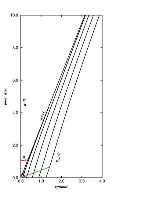
Figure 10: Field and streamlines for the conical $r$-self similar model of case (3), Table 3 and the following set of parameters: $x_{1}=-0.1,x_{2}=0.01$ and $E_{1}=-78.601635$, $E_{2}=-728.31337$, $C_{1}=-4.3231$, $C_{2}=D_{2}=0$, $D_{1}=-43.231$, $\theta_{\star}=65^{o}$, $\varphi_{\star}=75.784234^{o}$, $p_{\star}=-0.5$. In this case $V_{\phi}\propto R^{-1/2}$ on the equatorial plane while on the poloidal field/streamline $\alpha_{out}=2$, $B_{p}=V_{p}=0$. For large distances from the disk all lines with $\alpha>0$ go asymptotically to the line $\theta=\theta_{min}$.

Figure 11: The characteristic velocities of model (3) of Table 3 with conical asymptotical geometry are plotted in units of the z-component of the flow speed at the point $(\alpha=1,\theta=\pi/2)\,,V_{o}$ and the same parameters as in Fig. (10).

(3) Finally, in Figs. (10-11) the $r$-self similar model of case (3) in Table 3 gives a conical asymptotical geometry for a third set of the parameters ($x_{i}$, $E_{i}$, $C_{i}$, $D_{i}$), i=1,2 and $\theta_{\star}=65^{o}$, $\varphi_{\star}=75^{o}$, $p_{\star}=-0.5$. Note that now the solution exists only for $\theta>\theta_{min}$ where $\theta_{min}\approx 17.5^{o}$. When this value of $\theta$ is approached, $(M^{2}\,,G^{2})\rightarrow\infty$.

In all these four possibilities and along a given field/streamline, the outflow starts from the equator where $V_{\phi}\propto R^{-1/2}$ with a low subAlfvénic poloidal speed. This poloidal speed $V_{p}$ crosses the Alfvén conical surface at $\theta_{\star}$ in all cases. In the cylindrical case of Fig. (7), $V_{p}$ increases rapidly to a uniform value when collimation is achieved . The azimuthal speed $V_{\phi}$ on the other hand, drops with height in all cases, as rotational energy is transformed to poloidal kinetic energy. Finally, the azimuthal Alfvén speed is the strongest in the cylindrical case where the toroidal magnetic field is responsible for the ensuing final collimation.

4 Summary

In this paper we have examined a systematic way for constructing exact MHD solutions for plasma flows. The first assumption was to consider the ideal plasmas MHD equations for time-independent conditions, Eq. (1-2), without imposing the extra constraint of the frequently used polytropic assumption. Second, we confined our attention to axisymmetric situations in which case the poloidal magnetic and velocity fields can be expressed in terms of the magnetic flux function $A$ while several integrals exist, Eq. (4-5). In that case, besides $A$, a second natural variable is the Alfvén Mach number $M$, Eq. (3). We denoted by $G$ the cylindrical distance $\varpi$ of a poloidal streamline from the system’s symmetry axis, in units of the cylindrical distance of the Alfvén surface from the same axis, $\varpi_{\alpha}$. Third, we further confined our attention to transAlfvenic outflows in which case the regularization of the azimuthal components in Eq. (4-5) requires that the ratio of the two integrals of the total specific angular momentum in the flow $L(A)$ and corotation frequency $\Omega(A)$ is some function $\alpha(A)$ [as in Eq. (8)]. By introducing some reference scale $\varpi_{o}$ this function $\alpha$ is dimensionless, [as in Eq. (7) where $\varpi_{o}\equiv r_{\star}$]. Apparently ($M,\alpha$) is a rather convenient set of dimensionless variables for describing all physical quantities in the poloidal plane. For any set of orthogonal curvilinear coordinates suitable for describing axisymmetric problems, we may then convert their poloidal coordinates to ($M,\alpha$). Examples are, spherical coordinates [$r(M,\alpha),\theta(M,\alpha),\phi$], cylindrical coordinates [$z(M,\alpha),\varpi(M,\alpha),\phi$], toroidal coordinates [$u(M,\alpha),v(M,\alpha),\phi$], oblate/prolate spheroidal coordinates [$\xi(M,\alpha),\eta(M,\alpha),\phi$], paraboloidal coordinates, etc. Then, the distance from the symmetry axis of the outflow is $G(M,\alpha)$. In the present first study we made the simplifying fourth assumption that $G$ is independent of $\alpha$, $G=G(M)$ only. Finally, to re-establish the connection with the geometry of the problem and the particular set of the coordinates used, we made our fifth and final assumption that $M=M(\chi)$ (and $G=G(\chi)$), where $\chi=r$, or, $\chi=\theta$. This leads then to the two broad classes of meridionally and radially self-similar outflows. Needless to say that additional symmetries may in principle be considered, something which may be taken up in another connection (equilibria in tokamak geometries, etc).

After these five assumptions are well posed and with the help of a simple theorem, it is possible to (i) unify all existing exact solutions for astrophysical outflows (Tables 1,2 and 3) and (ii), to qualitatively sketch a few of them. With this method, the system of the coupled MHD equations reduces to a set of five ordinary differential equations for the dimensionless jet radius ($G$), the flow’s expansion factor or angle ($F$, or $\varphi$), the Alfvén Mach number ($M$) and the two pressure components ($P_{1}$ and $P_{0}$). The requirement that the solutions pass through the Alfvén critical point gives a condition relating the values of the expansion function or angle, Alfvén number slope and pressure component at this critical point. The Alfveń regularity conditions, Eqs. (138), (113) is similar to that discussed in Heyvarts & Norman (1989) and ST94.

As a byproduct of this construction, two representative models for radially and meridionally self-similar outflows, BP82 and ST94, respectively, have been generalized. In the former case of BP82, it is well known that the cold plasma solution is terminated at a finite height above the disk while the general case (3) in Table 3 extends all the way to infinity. Also, it is shown that the expressions of the MHD integrals which correspond to the ST94 model are only a special case of case (2) in Table 1.

Having in mind the ubiquitously observed collimated outflows from astrophysical objects, we paid more attention to the selfconsistently derived asymptotical shape of the streamlines. Of the various such asymptotic geometries derived, a prominent member seem to be the cylindrically collimated jet-type solutions, in accordance also with the conclusions of observations (Livio 1997), general theoretical arguments (Heyvaerts & Norman 1989) and recent numerical simulations (Goodson et al 1997). Another feature that appeared in the solutions is that cylindrical collimation may or may not be achieved with oscillations in the width of the jet (Vlahakis & Tsinganos 1997). Although in the examples analyzed here the amplitude of the oscillations is rather weak and the flow collimates rather smoothly, preliminary results show that cases also exist where it can become rather large and the final radius of the jet can be much smaller than the initial large cylindrical radius and corresponding opening angle. Finally, we should note that the pressure $P$ denotes the total pressure (including gas pressure, Alfvén waves pressure, radiative forces, etc). For example, the same formalism may be used also in radiation driven winds.

Appendix A functions of $R$

$$F=2-R\frac{G^{2^{\prime}}}{G^{2}}\equiv\frac{\partial\ln\alpha(R,\theta)}{\partial\ln R}\,.$$ (139)

$$f_{1}=-\frac{1}{G^{4}}\,,$$ (140)

$$f_{2}=-\frac{F^{2}-4}{4G^{2}R^{2}}\,,$$ (141)

$$f_{3}=-\frac{1}{G^{2}}\left(\frac{1-G^{2}}{1-M^{2}}\right)^{2}\,,$$ (142)

$$f_{4}=\frac{F}{2RG^{2}}M^{2^{\prime}}-\frac{1-M^{2}}{2RG^{2}}F^{{}^{\prime}}-\frac{\left(1-M^{2}\right)F\left(F-2\right)}{4R^{2}G^{2}}\,,$$ (143)

so,

$$F^{\prime}=\frac{F}{1-M^{2}}M^{2^{\prime}}-\frac{F\left(F-2\right)}{2R}-\frac{2RG^{2}}{1-M^{2}}f_{4}\,,$$ (144)

$$f_{5}=\frac{G^{4}-M^{2}}{G^{2}M^{2}\left(1-M^{2}\right)}\,,$$ (145)

$$f_{6}=-\frac{2}{G^{4}}M^{2^{\prime}}+\frac{2\left(1-M^{2}\right)\left(F-2\right)}{RG^{4}}\,,$$ (146)

$$f_{7}=\frac{2}{R^{2}G^{2}}M^{2^{\prime}}-\frac{\left(1-M^{2}\right)\left(F-2\right)\left(F+4\right)}{2R^{3}G^{2}}-\frac{F}{R}f_{4}\,,$$ (147)

$$f_{8}=-\frac{F-2}{R}f_{5}\,,$$ (148)

$$f_{9}=-\frac{\nu^{2}}{R^{2}M^{2}}\,.$$ (149)

Appendix B functions of $\theta$

$$H=2-\frac{G^{2^{\prime}}}{G^{2}}\equiv\frac{\partial\ln\alpha(R,\theta)}{\partial\ln\sin\theta}\,,$$ (150)

$$H=-2\frac{\sin\theta\sin\left(\varphi+\theta\right)}{\cos\theta\cos\left(\varphi+\theta\right)}=2-2\frac{\cos\varphi}{\cos\theta\cos\left(\varphi+\theta\right)}\,,$$ (151)

where the expansion angle $\varphi$ is the angle between the line and the equatorial plane, which is a function of $\theta$.

$$\frac{dG^{2}}{d\theta}=\frac{2G^{2}\cos\varphi}{\sin\theta\cos\left(\varphi+\theta\right)}\,,$$ (152)

$$h_{1}=-{\left(\sin^{2}\theta+\cos^{2}\theta{H^{2}\over 4}\right)\over G^{4}}=-\frac{\sin^{2}\theta}{G^{4}\cos^{2}\left(\varphi+\theta\right)}\,,$$ (153)

$$h_{2}=-\frac{1}{G^{2}}\left(\frac{1-G^{2}}{1-M^{2}}\right)^{2}\,,$$ (154)

$$h_{3}=\frac{G^{4}-M^{2}}{M^{2}G^{2}\left(1-M^{2}\right)}\,,$$ (155)

$$h_{4}=-\frac{\sin\theta}{GM^{2}}\,,$$ (156)

$$h_{5}=-\frac{\cos^{2}\theta}{2G^{4}}\left\{\left[H\left(1-M^{2}\right)\right]^{{}^{\prime}}+\right.$$

$$\left.\left(H-2\right)\left(1-M^{2}\right)\left(H-\tan^{2}\theta\right)\right\}\,,$$ (157)

or,

$$h_{5}=\frac{1-M^{2}}{G^{4}}\frac{\sin^{2}\theta}{\cos^{2}\left(\varphi+\theta\right)}\frac{d\varphi}{d\theta}-\frac{\sin^{2}\theta\sin\left(\varphi+\theta\right)}{G^{4}\cos\left(\varphi+\theta\right)}\frac{dM^{2}}{d\theta}-$$

$$\frac{1-M^{2}}{G^{4}}\frac{\sin\theta\cos\varphi\sin\left(\varphi+\theta\right)}{\cos^{2}\left(\varphi+\theta\right)}\,,$$ (158)

so,

$$\frac{d\varphi}{d\theta}=\frac{\sin\left(\varphi+\theta\right)\cos\left(\varphi+\theta\right)}{1-M^{2}}\frac{dM^{2}}{d\theta}+\frac{\sin\left(\varphi+\theta\right)\cos\varphi}{\sin\theta}+$$

$$\frac{\cos^{2}\left(\varphi+\theta\right)}{\sin^{2}\theta}\frac{G^{4}}{1-M^{2}}h_{5}\,.$$ (159)

References

• [1] Bardeen, J.M., Berger, B.K., 1978, ApJ, 221, 105
• [2] Biretta, T., 1996, in Solar and Astrophysical MHD Flows, K. Tsinganos (ed.), Kluwer Academic Publishers, 357
• [3] Blandford, R.D., Payne, D.G., 1982, MNRAS, 199, 883 (BP82)
• [4] Blandford, R.D., Rees, M.J., 1974, MNRAS, 169, 395
• [5] Burderi, L., King, A.R., 1995, MNRAS, 276, 1141
• [6] Burrows, C.J., et al, 1995, ApJ, 452, 680
• [7] Cao, X., 1997, MNRAS, 291, 145
• [8] Contopoulos, J., Lovelace, R.V.E., 1994, ApJ., 429, 139
• [9] Crane, P., Vernet, J., 1997, ApJ, 486, L91
• [10] Feldman, W.C., Phillips, J.L., Barraclough, B.L., Hammond, C.M. 1996, in Solar and Astrophysical MHD Flows, K. Tsinganos (ed.), Kluwer Academic Publishers, 265
• [11] Ferrari, A., Massaglia, S., Bodo, G., Rossi, P., 1996, in Solar and Astrophysical MHD Flows, K. Tsinganos (ed.), Kluwer Academic Publishers, 607
• [12] Ferreira, J., 1997, A&A, 319, 340
• [13] Ferreira, J., & Pelletier, G., 1995, A&A, 295, 807
• [14] Goodson, A.P., Winglee, R.M., Bohm, K.H., 1997, ApJ, 489, 199
• [15] Heyvaerts, J., Norman, C.A., 1989, ApJ, 347, 1055
• [16] Kafatos, M., 1996, in Solar and Astrophysical MHD Flows, K. Tsinganos (ed.), Kluwer Academic Publishers, 585
• [17] Konigl, A., 1989, ApJ, 342, 208
• [18] Li, Z.-Y, 1995, ApJ, 444, 848
• [19] Lima, J., Tsinganos, K., Priest, E., 1996, Astrophys. Letts. and Comms., 34, 281
• [20] Livio, M., 1997, in Accretion Phenomena and Related Outflows, D.T. Wickramasinghe, L. Ferrario, & G.V. Bicknel (eds.), ASP: San Francisco, 845.
• [21] Mirabel, I.F., Rodriguez, L.F., 1996, in Solar and Astrophysical MHD Flows, K. Tsinganos (ed.), Kluwer Academic Publishers, 683
• [22] Parker, E.N. 1958, ApJ, 128, 664
• [23] Pelletier, G., Pudritz, R.E., 1992, ApJ, 394, 117
• [24] Ray, T.P., 1996, in Solar and Astrophysical MHD Flows, K. Tsinganos (ed.), Kluwer Academic Publishers, 539
• [25] Sauty, C., Tsinganos, K., 1994, A&A, 287, 893 (ST94)
• [26] Trussoni, Tsinganos, K., E., Sauty, C., 1997, A&A, 325, 1099
• [27] Tsinganos, K.C., 1982, ApJ, 252, 775
• [28] Tsinganos, K., Trussoni, E., 1991, A&A, 249, 156
• [29] Tsinganos, K., Sauty, C., Surlantzis, G., Trussoni, E., Contopoulos, J., 1996, MNRAS, 283, 811
• [30] Vlahakis, N., Tsinganos, K., 1997, MNRAS, 292, 591
• [31] Weber, E.J., Davis, L.J. 1967, ApJ, 148, 217