Clustering of Ionizing Sources

Abstract

Using existing models for the evolution of clustering we show that the first sources are likely to be highly biased and thus strongly clustered. We compute intensity fluctuations for clustered sources in a uniform IGM. The strong fluctuations imply the universe was reheated and reionised in a highly inhomogeneous fashion.

Introduction

Fluctuations in the ionizing intensity during reionization result in temperature and ionization fraction fluctuations. This has important implications for the reheating and reionization history of the IGM. There are two contributing components:

${\bullet}$ IGM density fluctuations (variable optical depth)

${\bullet}$ Spatial distribution of ionizing sources

The second point is usually addressed by computing Poisson fluctuations in the ionizing intensity (fardal ,zuo ). Here we consider a hitherto neglected effect, the clustering of ionizing sources, and show that it is the dominant source of intensity fluctuations.

Modelling the Ionizing Sources

We work within the framework of the concordance cosmology of os95 :$(\Omega_{m},\Omega_{\Lambda},\Omega_{b},h,\sigma_{8h^{-1}},n)=(0.35,0.65,0.04,0.65,0.87,0.96)$. We parametrise our model of reionization with 3 relevant lengthscales:

$\bullet$Mean separation $n^{-1/3}$ The comoving number density of collapsed objects above a critical mass ${\rm M_{*}}$ is given by Press-Schechter theory: $n(z)=\Delta t\int_{M_{*}}^{\infty}\dot{n}_{PS}(M,z)dM$, where the creation rate of dark matter halos is given in sasaki . The critical mass $M_{*}$ is given by the Jeans mass after reheating, $M_{Jeans}\sim 10^{9}(1+z/10)^{-3/2}M_{\odot}$. Before reheating, it is given by the virial mass necessary for efficient atomic cooling $M_{cool}\sim 10^{8}(1+z/10)^{-3/2}M_{\odot}$ . The source lifetime is assumed to be $\Delta t\sim 10^{7}$ yrs, the characteristic timescale for both starbursts and quasars.

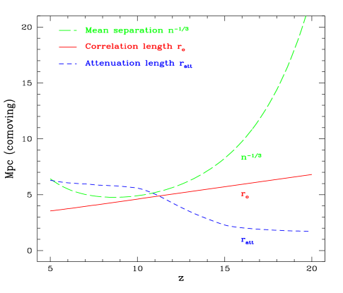
Figure 1: The evolution of various lengthscales with redshift. The increasing bias factor with redshift counteracts the fall of the linear growth factor, causing $r_{o}$ to remain almost constant. The downturn of $r_{atten}$ at low redshift is caused by the increased clumping of the gas, which shortens the recombination time.

$\bullet$ Attenuation length $r_{\rm atten}$ This is modelled as min($r_{strom},r_{life},r_{Lyman})$, where $r_{strom}$ is the Stromgren radius, $r_{life}$ is the radius of the volume ionized by a source during its lifetime, and $r_{Lyman}$ is the mean free path of photons bounded by the covering factor of Lyman limit systems. We assume values for the clumping of the IGM computed in go97 . The covering factor of Lyman limit systems is computed by assuming a mini-halo model (e.g.,abelmo ), and computing their abundance via Press-Schechter theory.

$\bullet$ Correlation length $r_{o}$ The evolution of the matter correlation function with redshift is given by integrating the power spectrum. We assume a linear bias model $\xi_{\rm hh}(r)=b^{2}\xi_{\rm mm}(r)$. Given the linear bias factor $b(M)$ as in mowhite , we then compute $b(M,z)$ by assuming linear theory and thus compute a number weighted bias factor at each epoch $\tilde{b}(z)$:

$$\tilde{b}(z)=\frac{\int_{M_{*}}^{\infty}b(M,z)n(M,z)dM}{\int_{M_{*}}^{\infty}n(M,z)dM}$$ (1)

The high bias means that the correlation length of halos is large, even though the correlation length of matter falls with redshift. For example, $\tilde{b}\sim 7$ at z=12, which leads to $r_{o}^{\rm halo}\sim 3.3{\rm Mpc}h^{-1}$ in comoving coordinates, only somewhat weaker than the clustering of objects seen today. We also calculate the evolution of the 3 and 4 point correlation functions, assuming standard hierarchical scaling relations, $\bar{\xi}_{N}(r)={\rm S}_{N}\bar{\xi}_{2}^{N-1}(r)$. Note that the $S_{N}$, although scale invariant, are a function of bias as well.

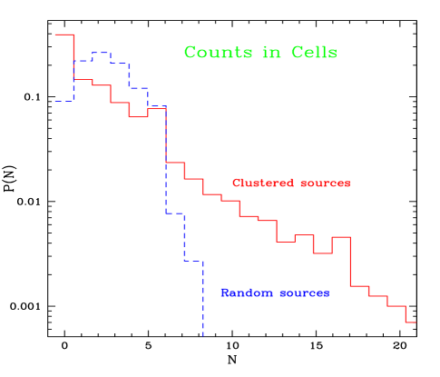
Figure 2: The probability distribution function of counts in cells at $z\sim 12$ for clustered and Poisson distributed sources, for a sphere of radius $r_{atten}\sim 4$ Mpc (comoving). The clustered case has a high N tail, where many low luminosity sources can mimic an ultra luminous source. Note also the greatly increased probability for N=0 (voids) in the clustered case.

To estimate the fluctuations in the radiation field, we conduct a Monte-Carlo simulation, in the spirit of fardal . We generate a mock catalog of ionizing sources in a box 150 Mpc comoving size at $z_{reion}\sim 12$. A fractal model soneira is used to lay down sources with specified 2, 3 & 4 point correlation functions, with appropriate modelling of the bias factors. This has the chief advantage of speed and convenience over using N-body simulations. It also does not suffer from mass resolutions effects in identifying halos. We verify that the 2 point correlation function and the 2nd, 3rd and 4th moments of counts in cells (which are directly related to the volume-averaged correlation functions, with corrections for shot noise) are correctly recovered. Luminosity is then randomly assigned to each source, assuming a Press-Schechter mass function, and a constant emissivity per unit mass, as given by haiman for their mini-quasar model. The ionizing flux at random points in the box is then computed, assuming each source ionizes out to a radius $r_{\rm atten}$. We thus compute the distribution function of the ionizing flux, as well as the two point correlation function $\xi_{JJ}(r)=<(J(0)-<J>)(J(r)-<J>)>/<J>^{2}$.

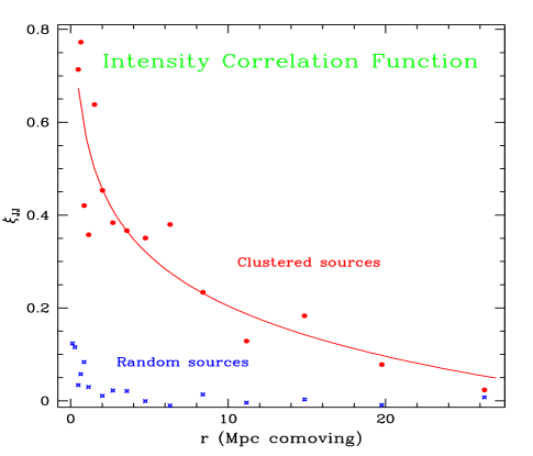
Figure 3: The two-point correlation function of ionizing intensity at $z\sim 12$ as a function of separation, assuming a sharp cutoff in ionizing flux at $r_{atten}$. In the clustered case, the radiation field displays correlations over large lengthscales.

Conclusions & Observational Implications

Clustering of ionizing sources produces a large dispersion in the luminosity of random cells. Clustered sources collectively mimic an ultra-luminous source. In addition, large voids exist where no ionizing sources are present. These are ionized by the percolation of ionizing radiation. Thus, large intensity fluctuations arise in the radiation field, which show coherence on large scales.

This has important observational implications. Emission line searches (e.g. in Ly$\alpha$ and H$\alpha$) at high redshift have a stronger signal due to the higher intensity fluctuations. Furthermore, CMB fluctuations due to Thomson scattering off electrons in moving ionized patches knox are enhanced, both due to the larger patch sizes and the spatial correlations of the ionized patches. Finally, uneven reheating provides a possible biasing mechanism.

Acknowledgements I thank my advisor, David Spergel, for his support and encouragement. I also thank Michael Strauss for helpful conversations.

References

- (1) Fardal M.A., & Shull, J.M. 1993, ApJ, 415, 524
- (2) Zuo L. 1992, MNRAS, 258, 45
- (3) Ostriker, J.P., & Steinhardt, P. 1995 Nature, 377, 600
- (4) Sasaki, S., 1994, PASJ, 46, 427
- (5) Gnedin, N., & Ostriker, J.P. 1997, ApJ, 486, 581
- (6) Abel, T., & Mo, H.J. 1998, ApJ 494, L151
- (7) Mo, H.J., & White, S.D.M. 1996, MNRAS 282, 347
- (8) Soneira, R.M. & Peebles, P.J.E 1978 AJ 83, 845
- (9) Haiman, Z., & Loeb, A. 1998, ApJ, 503, 505
- (10) Knox, L., Scoccimarro, R., Dodelson, S., 1998, Phys. Rev. Letters 81,2004