Weak Gravitational Lensing by Voids

Abstract

We consider the prospects for detecting weak gravitational lensing by underdensities (voids) in the large-scale matter distribution. We derive the basic expressions for magnification and distortion by spherical voids. Clustering of the background sources and cosmic variance are the main factors which limit in principle the detection of lensing by voids. We conclude that only voids with radii larger than $\sim 100$ $h^{-1}$ Mpc have lensing signal to noise larger than unity.

1 Introduction

Gravitational lensing remains a rapidly evolving field of study, with observational evidence now firmly established for the phenomena of strong, weak, and micro-lensing. Examples include multiple imaging of background quasars by foreground galaxies, weak distortion of background galaxy images by foreground galaxy clusters, and time-dependent enhancement of stellar brightness by underluminous objects in our own galaxy.

In each of these cases, the intervening matter between the source and observer acts as a converging lens, leading to image splitting, magnification, and distortion. In addition to mass concentrations, underdensities in the matter distribution—voids—also affect the propagation of light rays across cosmological distances. Over the last fifteen years, galaxy redshift surveys have revealed that a substantial fraction of the volume of the Universe is occupied by giant voids, quasi-spherical regions almost empty of luminous matter (e.g., de Lapparent et al. 1989, El-Ad et al. 1996, Da Costa et al. 1996). However, relatively little attention has been devoted to the possibility of detecting the gravitational lensing effects of voids. A light ray passing through an empty region is deflected away from the center of the void, since it is gravitationally attracted by the surrounding matter. This phenomenon is mentioned, although not discussed, in Hammer & Nottale (1986), in connection with a cluster model with a surrounding underdense shell. It is also discussed in the linear limit by Moreno & Portilla (1990), but they do not draw observational conclusions. The effects of large empty regions on light propagation in FRW universes has been extensively studied (e.g., Dyer & Roeder 1972; see Holz & Wald 1998 for a recent discussion), but these works did not focus on the detectability of individual voids via lensing.

In this paper we study gravitational lensing by large-scale voids and the possibility of its detection. Our motivations are several: First, voids are ubiquitous and large, accounting for some 80% of the volume of the Universe. It is in fact rather unlikely for a light ray from a distant source not to have passed through a void. Second, to understand the formation of such large voids we would like to know their matter content: are they nearly devoid of matter or only lacking bright galaxies? In principle, gravitational lensing can probe the matter content of voids. Third, some theories predict the formation of primordial voids, e.g., due to cosmic explosions (Ostriker & Cowie 1981; Yoshioka & Ikeuchi 1989) or primordial phase transitions (La 1991; Amendola & Occhionero 1993; Amendola et al. 1996). A search for such primordial structures could be pursued via their gravitational lensing signature. Fourth, “negative” masses, i.e., underdense regions, lead to new lensing phenomena that are of intrinsic theoretical interest.

Thus, we pose the following question: suppose a void of scale $R$ at redshift $z_{L}$ is identified in a galaxy redshift survey; can its lensing effect on background sources be measured and use to probe its matter density? Since this is an exploratory study, we consider a highly idealized model of a void, comprising a uniform spherical underdensity surrounded by a uniform overdense shell, in an otherwise homogenous universe. While only a starting point for a more realistic treatment, such a model captures the broad features found in numerical and analytical studies of voids growing via gravitational instability. We consider two techniques for detecting the lensing effect of voids, color-dependent angular density amplification (Broadhurst, Taylor & Peacock 1995, Broadhurst 1996) and aperture densitometry (Kaiser 1994, Schneider 1996). Unfortunately, we find that only voids with radii larger than 100 $h^{-1}$ Mpc can be individually detected via weak lensing; empty voids with radii $R=30$ $h^{-1}$ Mpc , characteristic of those seen in galaxy redshift surveys, have a lensing signal-to-noise ratio smaller than unity.

This paper is organized as follows: In Sec. $2$ we review the basic lens theory and apply it to lensing by spherical voids. The possibility of detecting the lensing effect using the color-dependent angular density amplification is investigated in Sec. $3$. In Sec. $4$ we apply the technique of aperture densitometry to the detection of voids. Our main conclusions are stressed out in Sec. $5$.

2 Lens theory and the spherical void

Here we review the basic features of gravitational lens theory and apply it to lensing by spherical voids. The lensing geometry in the case of voids is shown in Figure 1 . In the figure, L is the center of the void, S is a distant point source, and O the observer. The source is at distance $D_{OS}$ from the observer and $D_{LS}$ from the lens, and the distance between lens and observer is denoted by $D_{OL}$; these are angular diameter distances. Light rays from the source are ‘repelled’ by the lens center and are deflected by the angle $\hat{\alpha}$ (the deflection angle is negative for a matter underdensity). The angular separations between lens and image and between lens and source are denoted by $\hat{\theta}_{I}$ and $\hat{\theta}_{S}$. We note that a void can be thought of as an “extended negative mass lens” and some of its lensing properties can be obtained from that of a “negative point mass lens” in exactly the same way as the standard point mass lens is generalized to an extended lens (see, e.g., Schneider, Ehlers and Falco (1992)). Throughout this paper we adopt the “thin lens” approximation, applicable if the void radius $R$ is small compared with $D_{OL}$ and $D_{LS}$.

Now consider photons traveling in a weak gravitational field generated by a stationary bound system. If the deflection angle is small, it can be expressed as

$$\hat{\alpha}=\frac{2}{c^{2}}\int_{-\infty}^{\infty}\;\vec{\nabla}\Phi_{{}_{3D}}\;dl,$$ (1)

where $\Phi_{{}_{3D}}$ is the 3-dimensional Newtonian potential, satisfying the boundary conditions $\Phi=0$ and $\vec{\nabla}\Phi_{{}_{3D}}=0$ at infinity. Eqn. (1) follows from linearized general relativity; to lowest order, the integral is performed along the unperturbed (zero field) photon trajectory. In this approximation, $\hat{\alpha}$ is contained in the lens plane.

Figure 1: Void lensing geometry. Light rays from the source S are deflected by the lens L through angle $\hat{\alpha}$ and detected by observer O as an image at position I.

From Figure 1 we obtain the lens equation

$$\hat{\theta}_{S}=\hat{\theta}_{I}-\frac{D_{LS}}{D_{OS}}\hat{\alpha}~{}.$$ (2)

Introducing rescaled two-dimensional coordinates in the lens plane, $x_{j}=D_{OL}{\theta_{I}}_{j}$ and $y_{j}=D_{OL}{\theta_{S}}_{j}$, from Eqn.(2) we obtain

$$\frac{\partial y_{i}}{\partial x_{j}}=\delta_{ij}-\frac{D_{OL}D_{LS}}{D_{OS}}\frac{\partial\alpha_{i}}{\partial x_{j}}.$$ (3)

Using Eqn.(1), we can rewrite Eqn.(3) as

$$\frac{\partial y_{i}}{\partial x_{j}}=\delta_{ij}-\Psi_{ij},$$ (4)

where the 2-dimensional potential $\Psi$ is given by

$$\Psi=\frac{2}{c^{2}}\frac{D_{OL}D_{LS}}{D_{OS}}\int_{-\infty}^{\infty}\Phi_{{}_{3D}}dx_{3}$$ (5)

and $\Psi_{ij}\equiv\partial^{2}\Psi/\partial x_{i}\partial x_{j}$.

Since $\Phi_{{}_{3D}}$, $\vec{\nabla}\Phi_{{}_{3D}}$ $\rightarrow 0$ at infinity, from Poisson’s equation we find

$$\int_{-\infty}^{\infty}\left(\frac{\partial^{2}\Phi_{{}_{3D}}}{\partial{x_{1}}^{2}}+\frac{\partial^{2}\Phi_{{}_{3D}}}{\partial{x_{2}}^{2}}\right)dx_{3}\equiv 4\pi G\;\frac{\Sigma_{c}}{2}\nabla_{{}_{2D}}^{2}\Psi=4\pi G\;\Sigma,$$ (6)

where $\Sigma\equiv\int_{-\infty}^{\infty}\;\rho\;dx_{3}$ is the surface mass density, and the critical surface density $\Sigma_{c}$ is defined by

$$\Sigma_{c}\equiv\frac{c^{2}}{4\pi G}\frac{D_{OS}}{D_{OL}D_{LS}}.$$ (7)

Defining the convergence, $\kappa\equiv\Sigma/\Sigma_{c}$, it follows from Eqn.(6) that $\nabla_{{}_{2D}}^{2}\Psi=2\kappa.$

The shear is defined by

$$\gamma^{2}={\gamma_{1}}^{2}+{\gamma_{2}}^{2},$$ (8)

where $\gamma_{1}=\frac{1}{2}(\Psi_{11}-\Psi_{22})$ and $\gamma_{2}=\Psi_{12}=\Psi_{21}.$ From Eqn.(4), the Jacobian matrix of the lensing mapping, which describes its local properties, can be expressed as

$$A^{-1}=\pmatrix{1-\kappa-\gamma_{1}&-\gamma_{2}&\cr\vskip 3.0pt plus 1.0pt minus 1.0pt\cr-\gamma_{2}&1-\kappa+\gamma_{1}\cr}~{}.$$ (9)

Since lensing conserves surface brightness, the image magnification $\mu$ is given by the increase in image area due to convergence and shear,

$$\mu=\frac{1}{\det A^{-1}}=\frac{1}{(1-\kappa)^{2}-\gamma^{2}}.$$ (10)

We now apply this formalism to the spherical void lens. We model the void as a spherically symmetric matter distribution, with density excess $\delta\rho_{v}=\rho_{v}-\bar{\rho}$ given by

$$\delta\rho_{v}(r)=\left\{\begin{array}[]{lll}-\bar{\rho}\delta&\;\;{\rm for}\;\;\;\;\;\;\;\;\;\;\;r<R,&\\ \rho_{+}\delta&\;\;{\rm for}\;\;\;\;R<r<R+d,&\\ 0&\;\;{\rm for}\;\;\;\;\;\;\;\;\;\;\;\;r>R+d.&\end{array}\right.$$ (14)

Here, $\delta\rho_{v}/\bar{\rho}$ is the density contrast ($\delta<1$), and $\bar{\rho}$ is the mean energy density of the Universe. In Eqn.(11), $R$ is the void radius, and $d$ is the thickness of the surrounding mass shell. We assume that the mass excess in the shell exactly compensates the amount missing in the void, so $\rho_{+}$ and $\bar{\rho}$ are related by

$$\rho_{+}=\frac{\bar{\rho}}{\left(1+\frac{d}{R}\right)^{3}-1}~{}~{}.$$ (15)

In the limit $d\rightarrow\infty$ we obtain $\rho_{+}\rightarrow 0$, and we recover the simple uncompensated void.

It is convenient to define the impact parameter $b$ as the distance of closest approach of the unperturbed ray to the lens L. Introducing the scaled distances $\tilde{b}=b/R$ and $\tilde{d}=d/R$, the the surface mass density for the void model of Eqn.($11$) takes the form,

$$\Sigma(\tilde{b})=\left\{\begin{array}[]{lll}-2\bar{\rho}\delta R\;\left[\left(1-\tilde{b}^{2}\right)^{1/2}+\frac{\left(1-\tilde{b}^{2}\right)^{1/2}-\left((1+\tilde{d})^{2}-\tilde{b}^{2}\right)^{1/2}}{(1+\tilde{d})^{3}-1}\right]&\;\;\;{\rm for}\;\;\;\;\;\;\;\;\;\;\;\;\;\tilde{b}<1,&\\ 2\bar{\rho}\delta R\;\frac{[(1+\tilde{d})^{2}-\tilde{b}^{2}]^{1/2}}{(1+\tilde{d})^{3}-1}&\;\;\;{\rm for}\;\;\;\;\;\;1<\tilde{b}<1+\tilde{d},&\\ 0&\;\;\;{\rm for}\;\;\;\;\;\;\;\;\;\;\;\;\;\tilde{b}>1+\tilde{d}.&\end{array}\right.$$ (19)

The projected effective mass interior to the impact parameter $b$, ${\it M}(b)=2\pi\int_{0}^{b}a\Sigma(a)da$, is given by,

$${\it{M}(\tilde{b})=\left\{\begin{array}[]{lll}-\frac{M_{v}}{\tilde{d}^{3}+3\tilde{d}^{2}+3\tilde{d}}\left\{\left[(1+\tilde{d})^{2}-\tilde{b}^{2}\right]^{3/2}-(1+\tilde{d})^{3}(1-\tilde{b}^{2})^{3/2}\right\}&\;\;\;{\rm for}\;\;\;\;\;\;\;\;\;\;\;\tilde{b}<1,&\\ -\frac{M_{v}}{\tilde{d}^{3}+3\tilde{d}^{2}+3\tilde{d}}\left[(1+\tilde{d})^{2}-\tilde{b}^{2}\right]^{3/2}&\;\;\;{\rm for}\;\;\;\;1<\tilde{b}<1+\tilde{d},&\\ 0&\;\;\;{\rm for}\;\;\;\;\;\;\;\;\;\;\;\tilde{b}>1+\tilde{d},&\end{array}\right.}$$ (23)

where $M_{v}=\frac{4}{3}\pi\bar{\rho}\delta R^{3}$.

The magnification factor for a spherical void takes a simple form,

$$\mu=\left[1-\frac{\Sigma_{v}}{\Sigma_{c}}\frac{\tilde{M}(\tilde{b})}{{\tilde{b}}^{2}}\right]^{-1}\left[1-\frac{\Sigma_{v}}{\Sigma_{c}}\frac{d}{d\tilde{b}}\left(\frac{\tilde{M}(\tilde{b})}{\tilde{b}}\right)\right]^{-1},$$ (24)

where $\tilde{M}(\tilde{b})=M(\tilde{b})/M_{v}$ and $\Sigma_{v}=M_{v}/\pi R^{2}$.

In what follows we shall assume the Einstein-de Sitter universe ($\Omega_{m}=1$), in which the angular diameter distance takes a simple form,

$$D_{LS}=r(z_{L},z_{S})=c{H_{0}}^{-1}\frac{2}{1+z_{S}}\times\left[(1+z_{L})^{-1/2}-(1+z_{S})^{-1/2}\right],$$ (25)

and $D_{OL}=r(0,z_{L})$, $D_{OS}=r(0,z_{S})$.

The dimensionless quantity, $\Sigma_{v}/\Sigma_{c}$, which depends on $z_{S}$, $z_{L}$, $\delta$, and $R$, clearly sets the strength of gravitational lensing by voids. For instance, the magnification $\mu$ can be written in the limit of weak lensing as $\mu=1+(\Sigma_{v}/\Sigma_{c})f(\tilde{b},\tilde{d})$, where $f(\tilde{b},\tilde{d})$ is a function of order unity. For the Einstein-de Sitter model,

$$\frac{\Sigma_{v}}{\Sigma_{c}}=\frac{2R\delta D_{OL}D_{LS}}{(c/H_{0})^{2}D_{OS}}~{},$$ (26)

where $c/H_{0}=3000$ $h^{-1}$ Mpc is the Hubble radius. For voids at cosmological distances, $\Sigma_{v}/\Sigma_{c}\sim R\delta/cH_{0}^{-1}$; for example, for $R=50h^{-1}{\rm~{}Mpc}$, typically $\sum_{v}/\sum_{c}=.003-.005$. The ratio $\sum_{v}/\sum_{c}$ reaches at most 1% for giant voids of radius 100 $h^{-1}{\rm~{}Mpc}$.

Figure 2: The magnification $\mu$ versus scaled impact parameter $\tilde{b}$ in for two representative voids. The dashed curve corresponds to a compensated void with $\Sigma_{v}/\Sigma_{c}=0.005$ and $\tilde{d}=0.1$. The continuous curve is for an uncompensated void with $\Sigma_{v}/\Sigma_{c}=0.005$ and $\tilde{d}=2$.

In Fig. 2 we show the magnification $\mu$ as a function of the scaled impact parameter $\tilde{b}$ for two different types of voids. The dashed curve corresponds to a compensated void with $\Sigma_{v}/\Sigma_{c}=0.005$ and $\tilde{d}=0.1$. We also show the almost uncompensated void with $\Sigma_{v}/\Sigma_{c}=0.005$ and $\tilde{d}=2$. In the first case there is a peak at the void boundary ($\tilde{b}=1$) where images are always magnified ($\mu>1$). Images formed well inside the void ($\tilde{b}\ll 1$) are demagnified ($\mu<1$); for $\tilde{b}\geq 1+\tilde{d}$ there is no magnification. From Fig.1, the demagnification inside the void is higher in the case of an uncompensated void. In the weak lensing limit, $\kappa,\gamma\ll 1$, the magnification depends only on the convergence, $\mu\simeq 1+2\kappa$.

We now consider the image distortion induced by a void. A small circular source will be compressed by a factor $f_{r}=[1-(\kappa-\gamma)]^{-1}$ along the radial direction (away from the void center) and by a factor $f_{o}=[1-(\kappa+\gamma)]^{-1}$ along the tangential direction. For a spherical void, the convergence and shear can be expressed as

$$\kappa = \frac{1}{2}\frac{\Sigma_{v}}{\Sigma_{c}}\left[\frac{\tilde{M}(\tilde{b})}{\tilde{b}^{2}}+\frac{d}{d\tilde{b}}\left(\frac{\tilde{M}(\tilde{b})}{\tilde{b}}\right)\right]\,,$$

$$\gamma = \frac{1}{2}\frac{\Sigma_{v}}{\Sigma_{c}}\left[\frac{\tilde{M}(\tilde{b})}{\tilde{b}^{2}}-\frac{d}{d\tilde{b}}\left(\frac{\tilde{M}(\tilde{b})}{\tilde{b}}\right)\right]\,.$$ (27)

Figure 3: The convergence $\kappa$, shear $\gamma$, and ellipticity $q-1$ as a function of $\tilde{b}$, for $\Sigma_{v}/\Sigma_{c}=0.005$ and $\tilde{d}=0.1$.

As a measure of the image distortion, it is useful to define the induced ellipticity $q$ for a circular source,

$$q={\frac{1-(\kappa+\gamma)}{1-(\kappa-\gamma)}}\,.$$ (28)

For small $\kappa$ and $\gamma$, the ellipticity depends only on the shear, $q\simeq 1-2\gamma$. For negative shear, as is the case for voids, the radial image compression is smaller than the tangential compression; as a result, the images tend to be preferentially aligned in the radial direction. For positive mass concentrations (e.g., galaxy clusters), in the weak lensing limit the images are aligned tangentially. Since our void model is spherical, there is no rotation of the source image. In Fig. 3 we show $\kappa$, $\gamma$, and $q-1$ as a function of $\tilde{b}$, for $\Sigma_{v}/\Sigma_{c}=0.005$ and $\tilde{d}=0.1$. In Fig. 4, we display how randomly distributed circular background galaxies would appear in the case of void lensing (left panel) and in the case of an isothermal foreground cluster (right panel). In this figure, the source galaxies were all placed at the same redshift, and the distortion has been exaggerated to show the effect.

Figure 4: The appearance (ellipticity) of randomly distributed circular background galaxies in the case of void lensing (left panel) and for an isothermal lensing cluster (right panel).

3 Color-dependent density magnification

Since lensing changes the apparent brightness of a source, the galaxy number count vs. magnitude relation will be altered for sources behind a foreground lens; this effect has been proposed as a method for probing cluster masses (Broadhurst, Taylor & Peacock 1994, Broadhurst 1996, Van Kampen 1998). Weak lensing causes two opposing effects on the number density of background sources to fixed limiting magnitude. Compared to an unlensed sample, sources behind a void are demagnified by a factor $\mu<1$, resulting in fewer sources in a magnitude-limited survey. On the other hand, the radial deflection of light rays by the foreground void causes the background images to appear concentrated toward the line of sight to the lens, increasing their areal density by a factor $1/\mu$. For galaxies observed in the red, the latter effect dominates, leading to an enhancement in the number density of galaxies behind a void; for lensing by clusters, one expects a suppression of red background source counts.

Let $n_{0}(z)$ and $n_{b}(z)$ denote the number of galaxies per square degree per redshift interval in an unlensed sample and in a lensed sample with characteristic magnification $\mu$ centered on a void. Let $N_{0}(m)$ and $N_{b}(m)$ be the corresponding total number of galaxies per square degree in each sample to a given limiting magnitude $m$. Due to the two competing effects noted above, the counts are related by

$$n_{b}/n_{0}=\mu^{2.5s-1}~{},$$ (29)

where $s$ is the background galaxy count-magnitude slope, $s=d\log N_{0}/dm$. Broadhurst (1994,1996) reports that $s\approx 0.5$ in $B$ and $s\approx 0.15$ in $R$ at magnitudes $m\leq 23$. In the case of void lensing, except near the void boundary we have $\mu<1$, leading to an enhancement of galaxies observed in $R$ behind the lens than in the far field. In general, the slope $s$ varies with magnitude (Broadhurst, Taylor, & Peacock 1995). To simplify the analysis, we will assume $s$ is constant and use the value $s=0.15$ in numerical calculations. In fact this appears to be a good approximation up to $m_{lim}\sim 22$. For deeper surveys, the effective value of $s$ is larger and the effect we are estimating weaker. As will be clear from our results, even using this somewhat optimistic approximation, it is very difficult to obtain a high signal to noise ratio with this technique for voids.

Let us estimate the fractional variation $\delta_{b}=(N_{b}-N_{0})/N_{0}$ in the number count of red galaxies behind a void and compare it with various sources of noise. We assume that the unlensed redshift distribution of the sources in the sample is given by the normalized function $p(z)$, which we will specify below. In the weak lensing limit, the magnification $\mu=1+2\kappa$; therefore, for objects at fixed angular separation $\theta_{S}$ from the lens center at $z_{L}$

$$\delta_{b}=\int_{z_{L}}^{\infty}(5s-2)\kappa(z_{S},\theta_{S})p(z_{S})dz_{S}~{}.$$ (30)

There are four main sources of statistical error in this measurement: the variance $\sigma_{L}$ due to lensing by random density fluctuations along the line of sight, the Poisson noise $\sigma_{P}$ due to the finite number of sources, the variance $\sigma_{C}$ due to angular clustering of the source galaxies, and errors in the limiting apparent magnitude due to experimental errors and to uncertainties in the extinction/reddening correction. Let us start with the latter error in $m_{lim}$. If the galaxy counts scale as $N\sim 10^{sm_{lim}}$ with $s=0.15$, then it is easy to show that the error in the number counts from an error in $m_{lim}$ is smaller than the Poisson fluctuation only if $\Delta m_{lim}<0.03$. This is possible with current observational techniques; moreover, the amount of extinction can in principle be estimated with multi-color data and by correlating with dust maps (though uncertainties in this procedure can cause systematic errors). Therefore, in the following we will neglect the observational errors in $m_{lim}$ and focus on the other three sources of noise, which are inevitably present independent of the data quality. The total error in the number counts is therefore

$$\sigma_{N}^{2}=\sigma_{L}^{2}+\sigma_{P}^{2}+\sigma_{C}^{2}~{}.$$ (31)

The cosmic variance in the magnification field, the source of $\sigma_{L}$, is due to lensing by the random superposition of large-scale density fluctuations along the line of sight (this quantity is of considerable interest in its own right, and several lensing surveys are underway to detect it). The variance of the convergence field $\kappa$ has been evaluated in Bernardeau et al. (1996). For a matter power spectrum $P(k)$ and an angular top-hat window function $W_{2D}$ of size $\theta_{0}$, the variance of the convergence field is given in the Einstein-de Sitter universe by

$$\sigma_{\kappa}^{2}=(2\pi)^{-1}\int_{0}^{\infty}dz\;f(z)\;w^{2}(z)\;D_{+}^{2}(z)\int_{0}^{\infty}k\;P(k)\;W_{2D}^{2}[kr_{p}(z)\theta_{0}]\;dk~{},$$ (32)

where $r_{p}(z)=r(0,z)(1+z)$, $f(z)=dr_{p}/dz$, $D_{+}=(1+z)^{-1}$ is the growing mode of density fluctuations, and $w(z)$ is an “efficiency” function which depends on the source distribution (see Bernardeau et al. 1996):

$$w(z)=\frac{3}{2}(1+z)r_{p}(z)\int_{z}^{\infty}p(z^{\prime})\;[1-r_{p}(z)/r_{p}(z^{\prime})]\;dz^{\prime}.$$ (33)

For the density fluctuation power spectrum, we assume a cold dark matter (CDM) model with shape parameter $\Gamma=0.25$ and normalization $\sigma_{8}=0.6$ (White, Efstathiou & Frenk 1993); we use the Bardeen et al. (1986) transfer function. Using Eqn.(20) and the relation between $\mu$ and $\kappa$, we have

$$\sigma_{L}^{2}\approx(2-5s)^{2}\sigma_{\kappa}^{2}.$$ (34)

Another source of statistical error is the variance due to the angular clustering of the background sources. In terms of the present power spectrum $P(k)$, the variance of the density contrast in circular patches of angular radius $\theta$ can be obtained by writing the angular density contrast in an area $A=\pi\theta^{2}$ as

$$\delta(\theta)=A^{-1}\int_{A}d\Omega\int dz\;p(z)\;\delta(r,z)\;D_{+}(z)~{},$$ (35)

where $\delta(r,z)$ is the density field perturbation. This gives

$$\sigma_{C}^{2}=\langle[\delta(\theta)]^{2}\rangle=(2\pi)^{-1}\int_{0}^{\infty}dz\;p^{2}(z)\;D_{+}^{2}(z)\int_{0}^{\infty}k\;P(k)\;W_{2D}^{2}[kr_{p}(z)\theta_{0}]\;dk.$$ (36)

Finally, the Poisson noise is readily estimated as $\sigma_{P}^{2}=AN_{0}$, where $A$ is the area of the field in square degrees.

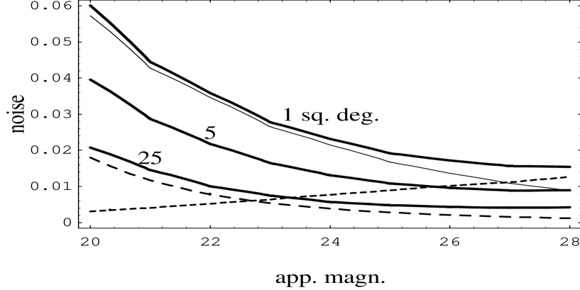
Figure 5: The various sources of error in the number of galaxies observed to limiting $R$ magnitude over a given area behind a void: Poisson noise $\sigma^{2}_{P}$ for 1 deg² field (long dashed curve); lensing variance $\sigma_{L}^{2}$ for 1 deg² (short dashed line); clustering variance $\sigma_{C}^{2}$ for 1 deg² (thin line); total variance $\sigma_{N}^{2}$ for 1 deg² (top thick curve), 5 deg² (intermediate thick curve), and 25 deg² (bottom thick curve).

Clearly, the Poisson and clustering contributions decrease with increasing depth of the sample, because the number of sources grows and the angular correlation function falls; by contrast, the lensing variance $\sigma_{L}^{2}$ increases with sample depth, because the number of lenses increases. Consequently, there is a depth for which $\sigma_{N}$ is a minimum. Of course, all the error contributions are smaller for a sample of larger angular size $\theta$. For a void at fixed redshift $z_{L}$, the lensing signal $\delta_{b}$ reaches a constant value at large depths, $z_{S}\gg z_{L}$, because the lensing effect is maximal for sources at $r(0,z_{S})\approx 2r(0,z_{L})$. We therefore expect the lens signal-to-noise to peak at a depth for which the noise is minimal; we confirm this below for the values of $z_{L}$ we have studied.

To estimate the signal-to-noise we must specify the source galaxy distribution $p(z)$. We consider two different models for the galaxy redshift distribution in a deep magnitude-limited sample. In the first, we follow Broadhurst, Taylor, & Peacock (1995) in assuming an evolving Schechter (1976) luminosity function,

$$\Phi(L,z)=\Phi^{*}(z)\exp[-L/L_{*}]~{},$$ (37)

with $\Phi^{*}(z)=0.02h^{-1}(1+z)^{2}(h^{-1}{\rm~{}Mpc})^{-3}$. The value $M^{*}=-21.5$ (for $h=1$) and a $K$-correction $K(z)=5\log_{10}(1+z)$ are appropriate values in the $R$ band. The fraction of galaxies in the redshift interval ($z,z+dz$) observed in a sample of $N_{0}$ galaxies with limiting apparent magnitude $m_{lim}$ (or limiting luminosity $L_{lim}(z_{S})$), is given by

$$p(z)dz=N_{0}^{-1}r^{2}_{p}(z)f(z)dz\int_{L_{lim}}^{\infty}\Phi(L,z)dL$$ (38)

where

$$L_{lim}=L_{\star}10^{0.4\left[M_{\star}-m_{lim}+25+5\log[(1+z_{S})^{2}r_{p}(z_{S})]\right]}~{}.$$ (39)

The second model provides a direct analytic parameterization of the redshift distribution based on a fit to galaxy redshift data (Efstathiou et al. 1991; Brainerd et al. 1995),

$$p(z)={3\over z_{0}^{3}\Gamma(1+3/\beta)}z^{2}e^{-(z/z_{0})^{\beta}}~{},$$ (40)

where $z_{0}$ and $\beta$ depend on the limiting magnitude. Empirically, $z_{0}=0.7$ and $\beta=2.6$ provides a good fit for $r_{lim}\sim 22$. For $r_{lim}\sim 22.5$, one can use $z_{0}=0.8$ and the same value of $\beta$. To obtain a typical estimate for deeper samples, we will use $z_{0}=1$ and $\beta=1.5$ (see, e.g., Schneider 1996); in this case, the median redshift of the sample is $\langle z\rangle\simeq 1.5$.

In Fig. 5 we show the sources of statistical error $\sigma_{P},\sigma_{C},$ $\sigma_{L}$, and $\sigma_{N}$ as a function of $m_{lim}$ (limiting $R$ magnitude) for various sample areas, assuming the redshift distribution of Eq. (38). As anticipated, the clustering variance dominates the other sources of error down to $m_{\lim}=26$, where the lensing variance becomes comparable. In Fig. 6a we plot the signal-to-noise ratio $S/N\equiv\delta_{b}\,/\sigma_{N}$ for void parameters $\tilde{d}=0.1$, $\tilde{b}=0.1$, and void radius $R=30$ $h^{-1}$ Mpc , as a function of void redshift $z_{L}$ and limiting magnitude $m_{lim}$, for a sample of area 25 deg². (As expected from Fig. 2, we find that the results do not change appreciably for $\tilde{d}<0.1$ and $\tilde{b}<0.1$.) It is evident that $S/N$ is well below unity at all limiting magnitudes and void redshifts. Since $S/N$ is linear in void radius, we conclude that only a huge, empty void of radius $R>100$ $h^{-1}$ Mpc would be detectable via lensing magnification. The same conclusion can be drawn from Fig. 6b, in which we plot $S/N$ versus $z_{L}$ for the same void parameters as above, but assuming the source redshift distribution of Eq. (40) with $z_{0}=1$ and $\beta=1.5$. The effect of several voids along the line of sight could accumulate to give a larger flux magnification, if no significant cluster is also intersected. However, as we have shown, for any given $m_{lim}$, there is a maximal contribution for a specific value of $z_{L}$, so that other voids far from this particular redshift are subdominant.

Figure 6: The signal-to-noise ratio $S/N$ for $\tilde{d}=0.1$, $\tilde{b}=0.1$ and void radius $R=30$ $h^{-1}$ Mpc as a function of $z_{L}$ and $m_{l}$, assuming $s=0.15$, for a sample of area of 25 deg² (left panel); the right panel shows $S/N$ versus $z_{L}$ for the same parameters, but assuming the redshift distribution of Eq. (40) with $z_{0}=1$ and $\beta=1.5$.

4 Aperture densitometry

In this section we apply the technique of aperture densitometry to the detection of voids. In this method, proposed by Kaiser ($1995$) and generalized by Schneider ($1996$), an upper limit to the projected mass of a lens inside an aperture is derived by measuring the shear inside an annulus. For rays passing well inside the void boundary, the convergence is negative; as a result, this technique will yield a lower limit to the void mass deficit.

Following Kaiser (1995) and Schneider (1996) we define the aperture mass,

$$m(\theta_{1},\theta_{2})=\int d^{2}x\;\kappa(\vec{\theta})\;w_{k}(\theta),$$ (41)

and we use the Kaiser compensated filter function,

$$w_{k}(\theta)=\left\{\begin{array}[]{lll}\frac{1}{\pi\theta_{1}^{2}}&\;\;{\rm for}\;\;\;\;\;\;\;\;\;\;\;\theta<\theta_{1},&\\ \frac{-1}{\pi(\theta_{2}^{2}-\theta_{1}^{2})}&\;\;{\rm for}\;\;\;\;\theta_{1}\leq\theta<\theta_{2},&\\ 0&\;\;{\rm for}\;\;\;\;\;\;\;\;\;\;\;\;\theta\geq\theta_{2},&\end{array}\right.$$ (45)

which satisfies the normalization condition $\int_{0}^{\theta_{2}}d\theta\;\theta\;w_{k}(\theta)=0$.

The aperture mass can be expressed in terms of the shear,

$$m(\theta_{1},\theta_{2})=\int d^{2}x\;\frac{\gamma_{t}(\vec{\theta})}{\theta^{2}}q(\theta),$$ (46)

where

$$\gamma_{t}(\vec{\theta})=-\gamma_{1}(\vec{\theta})\cos 2\phi+\gamma_{2}(\vec{\theta})\sin 2\phi,$$ (47)

is the tangential shear at the angular position $\vec{\theta}=(\theta\cos\phi,\theta\sin\phi)$ relative to the void center, and the function $q(\theta)$, defined by

$$q(\theta)=2\int_{0}^{\theta}d\theta^{\prime}\;\theta^{\prime}\;w_{k}(\theta^{\prime})-\;\;\theta^{2}w_{k}(\theta),$$ (48)

is equal to $\theta_{2}^{2}/\pi(\theta_{2}^{2}-\theta_{1}^{2})$ for $\theta_{1}\leq\theta<\theta_{2}$ and zero outside this region. Since $\langle\gamma_{t}\rangle=1/(2\pi)\int\gamma_{t}d\phi$, using (46) we recover the Kaiser $\zeta$-statistic (Kaiser 1995),

$$m(\theta_{1},\theta_{2})=\frac{2}{\left(1-\frac{\theta_{1}^{2}}{\theta_{2}^{2}}\right)}\int_{\theta_{1}}^{\theta_{2}}d\theta\,\frac{\langle\gamma_{t}\rangle}{\theta}=\overline{\kappa}(\theta<\theta_{1})-\overline{\kappa}(\theta_{1}<\theta<\theta_{2}).$$ (49)

Here, $\overline{\kappa}=\int d^{2}\theta\;\kappa/\int d^{2}\theta$ is the mean mass density within the aperture. We are considering axially symmetric voids, for which $\langle\gamma_{t}\rangle=\gamma_{t}=\gamma$. Further, since $\gamma<0$, and away from the void boundary $\overline{\kappa}$ is also negative, the shear inside the annulus can in principle be used to put a lower bound on the mass deficit (as compared with the mean mass density of the Universe) in the interior of a circle of radius $\theta_{1}$ around the center of the void.

In our computations we assume the source galaxies are distributed in redshift according to the normalized distribution function of Eqn.(40), and we take the values $z_{0}=1$ and $\beta=3/2$ as representative. The shear depends on the source redshift through the ratio $D_{LS}/D_{OS}$, so we define the source distance average ratio,

$$\left\langle\frac{D_{LS}}{D_{S}}\right\rangle=\int_{z_{L}}^{\infty}dz_{S}\;p(z_{S})\;\frac{D_{LS}}{D_{OS}}(z_{L},z_{S}).$$ (50)

A discretised estimator for the aperture mass (46) is given by

$$m=\frac{1}{n}\sum_{i}\varepsilon_{t}(\vec{\theta}_{i})\frac{q(\theta_{i})}{\theta_{i}^{2}}~{},$$ (51)

where $n$ is the source galaxy surface number density, and $\varepsilon_{t}$ is the tangential ellipticity of a galaxy at position $\vec{\theta}_{i}$. Since the intrinsic orientations of the source galaxies are random, in the absence of lensing $\langle m\rangle=0$. Squaring (51) and taking the expectation value, the dispersion of $m$ is (Schneider 1996)

$$\sigma_{d}^{2}=\frac{\sigma_{\varepsilon}^{2}}{2n^{2}}\sum_{i}\frac{q^{2}(\theta_{i})}{\theta_{i}^{4}},$$ (52)

where $\sigma_{\varepsilon}=\sqrt{\langle|\varepsilon|^{2}\rangle}$ is the dispersion of the intrinsic ellipticity distribution. The expectation value of the aperture mass estimator is

$$\langle m\rangle_{d}=\frac{1}{n}\sum_{i}\gamma_{t}(\vec{\theta}_{i})\frac{q(\theta_{i})}{\theta_{i}^{2}}~{}.$$ (53)

Performing an ensemble average of (51) and (52) over the probability distribution for the galaxy positions we get (Schneider 1996)

$$\langle m\rangle_{c}=2\pi\int_{\theta_{1}}^{\theta_{2}}d\theta\,\langle\gamma_{t}\rangle\,\frac{q(\theta)}{\theta}$$ (54)

and

$$\sigma_{c}^{2}(\theta_{1},\theta_{2})=\frac{\pi\sigma_{\varepsilon}^{2}}{n}\int_{\theta_{1}}^{\theta_{2}}d\theta\,\frac{q^{2}(\theta)}{\theta^{3}}.$$ (55)

Using $\bar{\rho}=\bar{\rho}_{0}\;(1+z_{L})^{3}$ and defining the scaled angle $\tilde{\theta}=\theta/\theta_{R}$, with $\theta_{R}\equiv R/D_{OL}$ the angular size of the void, we obtain the ensemble-average signal-to noise ratio (for the Einstein-de Sitter model)

$$S_{c}=\frac{|\langle m\rangle_{c}|}{\sigma_{c}(\theta_{1},\theta_{2})}\simeq 42\;\delta\;(1+z_{L})^{3}\;\left(\frac{0.2}{\sigma_{\varepsilon}}\right)\;\left(\frac{n}{30~{}{\rm arcmin}^{-2}}\right)^{1/2}\;\left(\frac{R}{20~{}h^{-1}{\rm Mpc}}\right)^{2}\;\left\langle\frac{D_{LS}}{D_{OS}}\right\rangle\;v(\tilde{d},\tilde{\theta}_{1},\tilde{\theta}_{2}),$$ (56)

where the dimensionless function

$$v(\tilde{d},\tilde{\theta}_{1},\tilde{\theta}_{2})\equiv\frac{\Sigma_{c}}{\Sigma_{v}}\frac{\tilde{\theta}_{1}\;\tilde{\theta}_{2}}{\sqrt{\tilde{\theta}_{2}^{2}-\tilde{\theta}_{1}^{2}}}\int_{\tilde{\theta}_{1}}^{\tilde{\theta}_{2}}d{\tilde{\theta}}\;\frac{|\gamma_{t}(\tilde{\theta},\tilde{d})|}{\tilde{\theta}}$$ (57)

is typically of order unity or less.

For example, for an empty void ($\delta=1$) of radius $R=30$ $h^{-1}$ Mpc and fractional shell thickness ${\tilde{d}}=0.1$ at redshift $z_{L}=0.1$, the signal-to-noise is $S_{c}\simeq 5$ for an ellipticity variance $\sigma_{c}=0.2$, aperture thickness $\Delta\theta=\theta_{2}-\theta_{1}=20$ arcmin (corresponding to $\Delta\tilde{\theta}=\tilde{\theta_{2}}-\tilde{\theta_{1}}=0.1$) and outer radius $\tilde{\theta_{2}}=0.7$. Thus, taking into account only the noise due to the dispersion of the intrinsic ellipticity distribution, we would conclude that voids can be detected with the aperture densitometry technique. However, voids do not exist in an otherwise homogeneous Universe: the mass is clustered on all scales, and the associated density perturbations cause random distortions of background galaxy images. The resulting cosmic variance in the aperture mass turns out to dominate over the intrinsic ellipticity dispersion and makes void lensing extremely difficult to detect. To see this, we note that the signal to noise ratio due to the intrinsic ellipticity distribution increases with the area of the sample: to achieve large signal to noise, it is necessary to increase the area of the annulus. However, as we show below, a larger sample area enhances the dispersion due to rms density perturbations (cosmic variance), with the result that only very large voids yield an observable lensing effect.

To estimate the cosmic variance noise we follow the method described in Schneider et al. (1998). Using the filter function of Eq.(45), we have

$$\langle M_{ap}^{2}(\theta_{1},\theta_{2})\rangle=2\pi\int_{0}^{\infty}ds\;s\,P_{k}(s)\,[I(s\theta_{1},s\theta_{2})]^{2},$$ (58)

where

$$I(s\theta_{1},s\theta_{2})=\frac{\theta_{2}}{s\pi\theta_{1}(\theta_{2}^{2}-\theta_{1}^{2})}\left(\frac{\theta_{2}}{\theta_{1}}J_{1}(s\theta_{1})-J_{1}(s\theta_{2})\right)~{},$$ (59)

with $J_{n}(x)$ denoting the Bessel function of the first kind. In Eq.(58), the quantity $P_{k}(s)$ is given by (Kaiser 1995, Schneider, et al. 1998),

$$P_{k}(s)=\frac{9}{4}\left({c\over H_{0}}\right)^{-3}\int_{0}^{\infty}dz\;\left\langle\frac{D_{LS}}{D_{OS}}\right\rangle(z)\;(1+z)^{-\frac{3}{2}}\;P_{0}(s/r(0,z)),$$ (60)

where $P_{0}(k)$ is the mass power spectrum. In our computation we use the non-linear CDM power spectrum (Hamilton, et al. 1991, Peacock & Dodds 1994,1996) with the Bardeen et al. (1986) transfer function, with shape parameter $\Gamma=0.25$ and normalized such that $\sigma_{8}=0.6$. The ratio between the cosmic variance and intrinsic ellipticity distribution contribution to the noise is (Schneider et al. 1998):

$$\rho=1500\pi\;\left(\frac{0.2}{\sigma_{\varepsilon}}\right)^{2}\;\left(\frac{n}{30~{}{\rm arcmin}^{-2}}\right)\;\langle M_{ap}^{2}(\theta_{1},\theta_{2})\rangle\;\left(\frac{\theta_{1}}{{\rm arcmin}}\right)^{2}\left(1-\frac{{\theta_{1}}^{2}}{{\theta_{2}}^{2}}\right)~{}.$$ (61)

The total aperture densitometry signal to noise ratio is then

$$\frac{S}{N}=\frac{S_{c}}{\sqrt{1+\rho^{2}}}~{}.$$ (62)

Figure 7: Aperture densitometry signal to noise ratio as a function of void redshift $z_{L}$, for an empty ($\delta=1$) void of radius $R=30h^{-1}$ Mpc and shell thickness $\tilde{d}=0.1$, assuming a density of background galaxies $n=30$ arcmin ^-2 with ellipticity dispersion $\sigma_{\varepsilon}=0.2$, evaluated at an outer angular radius $\tilde{\theta}_{2}=0.7$, and assuming a $\Gamma=0.2$ non-linear CDM power spectrum for the mass fluctuations. Results are shown for aperture width $\Delta\theta\equiv\theta_{2}-\theta_{1}\simeq 20$ (dot dashed), $2$ (solid), and $0.2$ arcmin (dashed) (corresponding to $\Delta\tilde{\theta}=0.1,\;0.01$, and $10^{-3}$). The long dashed curve shows results for the same model parameters but for a void of radius $R=100$ $h^{-1}$ Mpc and aperture $\Delta\tilde{\theta}=10^{-4}$.

In Fig. $7$ we plot the aperture densitometry signal to noise ratio as a function of void redshift $z_{L}$ for a void of radius $R=30$ $h^{-1}$ Mpc . We also show results for $R=100$ $h^{-1}$ Mpc , and aperture $\Delta\tilde{\theta}=10^{-4}$. This shows that very large void radii are required to achieve a signal to noise ratio larger than unity. We conclude that the void lensing signal for individual objects is quite difficult to detect via aperture densitometry, due to the large contribution of cosmic variance.

5 Summary and discussion

We have studied two methods for detecting weak lensing by large-scale voids in the matter distribution, color-dependent density magnification and aperture densitometry. We have found that only voids larger than $R\sim$ 100 $h^{-1}$ Mpc have a chance of being observed via lensing. In both cases, the limiting factor is clustering: for density magnification, the problem is angular clustering of the background sources; for aperture densitometry, the limit is set by lensing due to other clustered mass along the line of sight.

We note that the model studied here is highly idealized. In particular, we have assumed that a single void lens dominates the distortion and amplification along the line of sight, while typical light rays from high-redshift sources will in fact traverse a number of voids. On the other hand, if voids are ubiquitous, their mean cumulative effects should be described by the large-scale power spectrum, which we have taken into account via the cosmic variance noise. Our study therefore should be considered as applying to the detectability of individual, relatively rare, large, nearly empty voids embedded in a matter distribution otherwise described by a CDM-like power spectrum. The existence of such large voids in the galaxy distribution is a question that should be addressed by the next generation of large redshift surveys, including the Sloan Digital Sky Survey and the Two Degree Field Survey.

References

Amendola L. & Occhionero F. , 1993, Ap. J., 413, 39.

Amendola L. et al., 1996, Phys. Rev. D54, 7150.

Bardeen J. M., Bond J. R., Kaiser N., Szalay A. S., 1986, Ap. J., 304, 15.

Bernardeau F. , Van Waerbeke L., Mellier Y., 1997, A& A, 322, 1.

Broadhurst T. J., Taylor A. N. & Peacock J. A., Ap. J., 1995, 438, 49.

Broadhurst T. J., 1996, “Gravitational ‘Convergence’ and Galaxy Cluster Masses”- astro-ph/9511150.

da Costa L. N. et al. 1996, Ap. J., 468, L5.

de Lapparent V., Geller M., & Huchra J., 1989, Ap. J., 343, 1.

Dyer, C. C. & Roeder R. C. 1972, Ap. J., 174 , L115.

El-Ad H., Piran T. and da Costa L. N., 1996, Ap. J., 462, L13.

El-Ad H., Piran T. and da Costa L. N., 1997,MNRAS, 287, 790.

Hamilton A. J. S., Kumar P., Lu E., Matthews A., 1991, Ap. J., 374, L1.

Hammer F. & Nottale L., 1986, A& A, 167, 1.

Holz D. & Wald R. 1998, Phys. Rev. D58, 063501.

Kaiser N., 1995, Ap. J., 439, L1.

La D., 1991, Phys. Lett. B 265, 232.

Moreno J. & Portilla M., 1990, Ap. J., 352, 399.

Ostriker J. P. & Cowie L.N., 1981, Ap. J., 243, L127.

Peacock J. A., Dodds S. J., 1994, MNRAS, 267, 1020.

Peacock J. A., Dodds S. J., 1996, MNRAS, 280, L19.

Schechter P., 1976, Ap. J., 203, 297.

Schneider P., 1996, MNRAS, 283, 837.

Schneider P., Ehlers J. & Falco E. E., 1992,Gravitational Lenses, Springer: New York.

Schneider P., van Waerbeke L., Jain B. and Kruse G., 1998, MNRAS, 296, 873.

Van Kampen E., 1998, astro-ph/9807305

Yoshioka S. and Ikeuchi S., 1989, Ap. J., 341, 16.

White S. D. M., Efstathiou G. and Frenk C. S., 1993, MNRAS. 262,1023.