3D Simulation of the Gas Dynamics in the Central Parsec of the Galaxy

R.F. Coker¹ Fulvio Melia²

Abstract

It is thought that many characteristics of the gaseous features within the central parsec of our Galaxy, are associated with the accretion of ambient plasma by a central concentration of mass. Using a 3D hydrodynamical code, we have been simulating this process in order to realistically model the gaseous flows in the center of our Galaxy. In the most recent simulation, we have taken into account the multi-point-like distribution of stellar wind sources, as well as the magnetic heating and radiative cooling of these stellar winds. As expected, we find that the structure of the flow is significantly different from that due to a uniform medium. We also investigate the possibility that Sgr A* is due to a distributed mass concentration instead of the canonical point mass of a black hole. We discuss the physical state of the accreting gas and how our results suggest that Sgr A* is unlikely to be associated with a “dark cluster”.

Physics Department, The University of Arizona, Tucson, AZ 85721, USA

Physics Department and Steward Observatory, The University of Arizona, Tucson, AZ 85721, USA

¹¹footnotetext: NASA GSRP Fellow.²²footnotetext: Presidential Young Investigator.

1. Introduction

The hydrodynamics of the interstellar medium (ISM) within the central parsec of the Galaxy has long been thought to be dominated by the gravitational potential due to a central mass concentration (for a review, see Mezger, Duschl, & Zylka, 1996). For example, the Western Arc, one of the dominant kinematic features of the region, appears to be in circular rotation about Sgr A*, a unique compact radio source whose lack of proper motion suggests it lies at the dynamical heart of the Galaxy (Roberts & Goss, 1993; Backer, 1994). Stellar motions (Genzel, et. al., 1997), gas kinematics (Herbst, et. al., 1993), and velocity dispersion measurements (Eckart & Genzel, 1998) together suggest the presence of $\sim 2.6\times 10^{6}M_{\odot}$ of dark mass located within $\sim.01$ parsecs of Sgr A*. Note that the Galactic center (GC) is at a distance of $\sim 8$ kpc so that $1$ arcsecond $\sim 0.04$ parsecs.

However, showing that the GC must contain a centralized dark mass concentration does not necessarily imply that it is in the form of a single compact object nor does it imply that Sgr A* must be associated with it. Stellar kinematic arguments (Genzel et. al., 1996) rule out a distribution of neutron stars or white dwarfs. One possibility is that the dark mass distribution consists of $\sim 10M_{\odot}$ black holes; cluster evolution calculations (Lee, 1995) have shown that this is at least feasible although stability arguments (Maoz, 1998) suggest the cluster lifetime would be $\sim 10^{8}$ years, considerably less than the age of the Galaxy. In this paper, we wish to determine if, stability arguments aside, the spectrum of Sgr A* could be due to a plasma trapped within the potential well of a dark cluster of arbitrary objects.

In addition to large scale gaseous features, there is ample evidence for the existence of rather strong stellar winds in and around Sgr A* itself. The key wind sources appear to be the cluster of mass-losing, blue, luminous stars comprising the IRS 16 assemblage, located within several arcseconds of Sgr A*. A variety of observations over the years (for a review see Morris & Serabyn, 1996) provide clear evidence of a hypersonic wind, with a velocity of $v_{w}\sim 500-1000$ km s^-1, a number density $n_{w}\sim 10^{3-4}$ cm^-3, and a total mass loss rate $\dot{M}_{w}\sim 3-4\times 10^{-3}M_{\odot}~{}$ yr^-1 pervading the inner parsec of the Galaxy. If the dark matter is distributed, it is likely that a portion of this wind is captured by the dark compact cluster and that it settles within the cluster’s potential well. Although the potential well of a cluster does not include a cusp such as that due to a black hole, the trapped plasma might conceivably still account for at least some of Sgr A*’s radiative characteristics.

In §2 we discuss the simulation of the gas flow through a distributed dark mass cluster. In §3 we describe the resulting spectrum and present some preliminary semi-analytical spectral calculations based on Sgr A* being a point mass while in §4 we summarize our analysis.

2. The 3D Hydrodynamical Model

In the classical Bondi-Hoyle scenario (Bondi & Hoyle, 1944), the mass accretion rate for a uniform hypersonic adiabatic gas flowing past a centralized mass is

\dot{M}_{BH}=\pi{R_{A}}^{2}m_{H}n_{w}v_{w}\;,

(1)

where $R_{A}\equiv 2GM/{v_{w}}^{2}$ is the accretion radius and $M$ is the mass of the centralized object(s). At the GC, for the conditions described in the Introduction, we would therefore expect an accretion rate $\dot{M}_{BH}\sim 10^{21-22}$ g sec^-1, with a capture radius $R_{A}\sim 0.01-0.02~{}$ pc. Since this accretion rate is sub-Eddington for a $\sim$ one million solar mass concentration, the accreting gas is unimpeded by the escaping radiation field and is thus essentially in hydrodynamic free-fall starting at $R_{A}$ . Our initial, simplistic, numerical simulations of this process, where we assume a point object and uniform flow (Ruffert & Melia, 1994; Coker & Melia, 1996) have verified these expectations.

2.1. The Stellar Wind Sources

The GC wind, however, is unlikely to be uniform since the winds from many stars contribute to the mass ejection. We assume that the early-type stars enclosed (in projection) within the Western Arc, the Northern Arm, and the Bar produce the observed wind. Thus far, 25 such stars have been identified (Genzel, et. al., 1996), though the stellar wind characteristics of only 8 have been determined from their He I line emission (Najarro, et. al., 1997); the relavant characteristics of these 25 stars are summarized in Table 1. Two sources, IRS 13E1 and IRS 7W, seem to dominate the mass outflow with their high wind velocity ( $\sim 1000$ km sec^-1) and a mass loss rate of more than $2\times 10^{-4}\;M_{\odot}$ yr^-1 each. Unfortunately, the temperature of the stellar winds is not well known, and so for simplicity we have assumed that all the winds are Mach 30; this corresponds to a temperature of $10^{4-5}$ K. In addition, for the sources that are used in these calculations, their location in $z$ (i.e., along the line of sight) is determined randomly with the condition that the overall distribution in this direction approximately matches that in $x$ and $y$ .

Table 1.: Parameters for Galactic Center Wind Sources

Star	x^a (arcsec)	y^a (arcsec)	z^a (arcsec)	v (km sec^-1)	$\dot{M}({10}^{-5}\;M_{\odot}$ yr^-1)
IRS 16NE	-2.6	0.8	5.5	550	9.5
IRS 16NW	0.2	1.0	7.3	750	5.3
IRS 16C	-1.0	0.2	-7.1	650	10.5
IRS 16SW	-0.6	-1.3	4.9	650	15.5
IRS 13E1	3.4	-1.7	-1.5	1000	79.1
IRS 7W	4.1	4.8	-5.1	1000	20.7
AF	7.3	-6.7	8.5	700	8.7
IRS 15SW^b	1.5	10.1		700	16.5
IRS 15NE^b	-1.6	11.4		750	18.0
IRS 29N^c	1.6	1.4	3.5	750	12.9
IRS 33E^c	0.0	-3.0	1.5	750	12.9
IRS 34W^c	3.9	1.6	-6.4	750	12.9
IRS 1W^c	-5.3	0.3	7.8	750	12.9
IRS 9NW^cd	-2.5	-6.2	-3.8	750	12.9
IRS 6W^c	8.1	1.6	3.6	750	12.9
AF NW^cd	8.3	-3.1	-2.1	750	12.9
BLUM^b	9.2	-5.0
IRS 9S^b	-5.5	-9.2
Unnamed 1^b	1.3	-0.6
IRS 16SE^b	-1.4	-1.4
IRS 29NE^b	1.1	1.8
IRS 7SE^b	-2.7	3.0
Unnamed 2^b	3.8	-4.2
IRS 7E^b	-4.2	4.9
AF NWW^b	10.2	-2.7

The sources are assumed to be stationary over the duration of the simulation. The stars without any observed He I line emission have been assigned a wind velocity of $750$ km sec^-1 and an equal mass loss rate chosen such that the total mass ejected by the 14 stars used here is equal to $3\times 10^{-3}\;M_{\odot}$ yr^-1. Note that although we have matched the overall mass outflow rate to the observations, we have only used 14 of the 25 stars in the sample. There are two principal reasons for this: (1) stars further away than 10 arcsec (in projection) from Sgr A* are outside of our volume of solution and therefore could not be included, and (2) due to our computational resolution limits, we needed to avoid excessively large local stellar densities.

In a complex flow, generated by many wind sources, the wind velocity and density are not uniform, so the accretion radius is not independent of angle. To set the length scale for the simulation, we shall therefore adopt the value $R_{A}=.018$ pc (for which 1^′′ = 2.3 $R_{A}$ ) as a reasonable mean representation of this quantity.

2.2. The Dark Cluster Potential

We wish to study the emission characteristics of a hot, magnetized plasma “trapped” within the dark cluster’s gravitational potential well. Following Haller & Melia (1996), we will represent the gravitational potential of the dark cluster with an “ $\eta$ -model” (Tremaine, et. al., 1994). This function represents an isotropic mass distribution with a single parameter. We here restrict our examination to the case $\eta=2.5$ since this provides the closest approximation to a King model that is physically realizable (i.e., a nonnegative distribution function). We scale the mass so that $2\times 10^{6}\;M_{\odot}$ are enclosed within $0.01$ pc and the total integrated mass of the dark cluster is $2.7\times 10^{6}\;M_{\odot}$ . Thus, writing $r$ in units of $R_{A}$ we get for the enclosed mass as a function of $r$ ,

M_{\eta}(r)=2.7\times 10^{6}\left({{13.84r}\over{1+13.84r}}\right)^{5/2}\;M_{\odot}\;.

(2)

A more recent assessment of the enclosed mass (Genzel, et. al., 1997) places a yet more rigorous constraint on the possibility of a distributed dark matter component. These newer observations may indeed invalidate the idea that any realistic stable distribution of objects can account for the observed gravitational potential.

2.3. The Hydrodynamics Code

We use a modified version of the numerical finite difference algorithm ZEUS, a general purpose code for MHD fluids developed at NCSA (Stone & Norman, 1992; Norman, 1994). The code was run on the massively parallel Cray T3E at NASA’s Goddard Space Flight Center under the High Performance Computing Challenge program. Zone sizes are geometrically scaled by a factor of 1.02 so that the central zones are $\sim 20$ times smaller than the outermost zones, mimicking the “multiply nested grids” arrangement used by other researchers (e.g., Ruffert & Melia, 1994). This allows for maximal resolution of the central region (within the computer memory limits available) while sufficiently resolving the wind sources and minimizing zone-to-zone boundary effects. The total volume is $(40R_{A})^{3}$ or $\sim(0.7$ pc $)^{3}$ with the center of the spherically symmetric dark cluster distribution being located at the origin.

The density of the gas initially filling the volume of solution is set to a small value and the velocity is set to zero, while the internal energy density is chosen such that the initial gas temperature is $\sim 10^{2}$ K. Free outflow conditions are imposed on the outermost zones and each time step is determined by the Courant condition with a Courant number of 0.5. The 14 stellar wind sources are modeled by forcing the velocity in 14 subregions of 125 zones each to be constant with time while the densities in these subvolumes are set so that the total mass flow into the volume of solution from each source is given by Table 1. Also, the magnetic field of the winds is assumed to always be at equipartition with the thermal energy density. The angular momentum and mass accretion rates are calculated by summing the relevant quantity in zones located within $0.1R_{A}$ of the origin.

We assume the magnetic field is perfectly tangled and thus ignore the effects of the magnetic field on the large scale kinematics. We take the medium to be an adiabatic polytropic gas, with $\gamma=5/3$ . Building on previous work (Melia, 1994; Coker & Melia, 1997), we have included a first order approximation to magnetic dissipative heating as well as an accurate expression for the cooling due to magnetic bremsstrahlung, thermal bremsstrahlung, line emission, radiative recombination, and 2 photon continuum emission for a gas with cosmic abundance. For magnetic heating, we assume that the magnetic field never rises above equipartition. If compression and flux conservation would otherwise dictate a magnetic field larger than the equipartition value, the field lines are assumed to reconnect rapidly, converting the magnetic field energy into thermal energy, thereby re-establishing equipartition conditions. The cooling function includes a multiple-Gaussian fit to the relevant cooling emissivities provided by N. Gehrels (see Gehrels & Williams, 1993, and references cited therein), though with the thermal bremsstrahlung portion supplanted with more accurate expressions that are valid over a broader range of physical conditions and with the inclusion of magnetic bremsstrahlung. For details on the cooling expressions used in the hydrodynamics code as well as the spectrum calculations below, see Melia & Coker (1999). Note that cooling due to Comptonization and any pair production have not yet been included since they are not thought to be significant in the vicinity of Sgr A*. Also, it is assumed that the optical depth is small throughout the volume of solution.

2.4. Results of the 3D Simulation

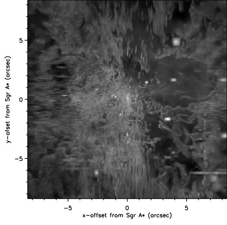
Refer to caption — Figure 1.: The line-of-sight integrated emissivity along the $z$ -axis.

The integrated emissivity along the line-of-sight, at $\sim$ 1450 years after the start of the simulation, is shown in Figure 1. The grey scale is logarithmic with solid white corresponding to a frequency-integrated intensity of $\sim 1.1\times 10^{5}$ erg cm^-2 s^-1 steradian^-1, and black corresponding to $\sim 1\times 10^{-2}$ erg cm^-2 s^-1 steradian^-1. Sgr A* is located at the center of the image. Of particular interest in this image is the appearance of streaks of high-velocity, high-density gas (“streamers”) that are very reminiscent of features, such as the so-called “Bullet” seen near the Galactic center (Yusef-Zadeh, et al. 1996). In our simulation, these structures are produced predominantly within the wind-wind collision regions, and in the future, we shall consider in greater detail the possibility that the observed high-velocity gas components near Sgr A* are produced in this fashion. Note the dominant role played by IRS 13E1 to the lower right of the compact radio source.

After reaching equilibrium several sound crossing times ( $\sim 1000$ years) after the start of the simulation, the enclosed mass and energy begin to fluctuate aperiodically on time scales of less than a few decades and with an amplitude of up to $50\%$ , reflecting the turbulent cell nature of the flow in and out of the central region. Typically $2.7\times 10^{-3}\;M_{\odot}$ of gas is trapped within the cluster at any given time. Also, although the gas is generally supersonic, with most of the energy in kinetic form, the thermal energy can be boosted rather suddenly when the enclosed magnetic field energy is dissipated. This occurs when strong shocks pass through the central region; the shocks compress the field sufficiently to the point where it reaches, or even surpasses, equipartition and dissipation ensues.

3. The Spectrum of Sgr A*

3.1. The Spectrum due to a Dark Cluster

In order to calculate the observed continuum spectrum, we assume that the observer is positioned along the negative $z$ -axis at infinity and we sum the emission from all zones that are located at a projected distance, $R_{xy}$ , of less than $0.1\,R_{A}$ . Since the size of Sgr A* (at $\lambda$ 7 mm) is $\approx 10^{12-13}$ cm (Bower & Backer, 1998) and the smallest cell size in our simulation is $7\times 10^{14}$ cm, in order to minimize the inaccuracy due to numerical fluctuations, we have calculated the spectrum from a central region roughly $10$ times this size ( $0.1R_{A}$ ), to include at least $100$ zones. Thus clearly our predicted spectrum constitutes an upper limit to the actual emission expected from Sgr A*. At the temperature and density that we encounter here, the dominant components of the continuum emissivity are electron-ion and electron-electron bremsstrahlung; we ignore line emission in these spectral calculations.

As discussed in Melia (1998), the density in the central region reaches a peak value of roughly $10^{8}$ cm^-3 and the temperature is never greater than about $10^{8}$ K. Thus, since electrons begin to emit significant synchrotron radiation only above a few times $10^{9}$ K, the gas can only emit cyclotron radiation. However, the cyclotron emissivity is insignificant compared to bremsstrahlung so that the final spectrum, as shown in Figure 2, is a bremsstrahlung spectrum that,in the radio, falls more than 4 orders of magnitude short of the observed luminosity of Sgr A* (compare with Figure 6b in Melia, 1998). Figure 2 shows spectra for 3 points in time during the 3D hydrodynamical simulation. The solid, dotted, and dashed curves are at approximately 1200, 1300, and 1400 years, respectively, after the start of the simulation. The flattening of the density, temperature, and magnetic field profiles is a direct consequence of the shallowness of the dark cluster potential compared to the steep potential gradient encountered by gas falling into a black hole. The high-energy shoulder of the emission shown in Figure 3 is characteristic of the highest temperature $T_{max}$ ( $\sim 10^{8}$ K) attained by the gas and is consistent with the brightness temperature limit associated with Sgr A*. Similarly, the X-ray and $\gamma$ -ray emission is significantly below the observed upper limits (Predehl & Truemper, 1994; Goldwurm, et. al., 1994).

3.2. The Spectrum due to a Black Hole

Although we have not yet run a 3D hydrodynamical simulation using the gravitational potential due to a point mass, we have undertaken semi-analytical calculations that improve upon earlier work (Melia, 1994). Although details will be presented elsewhere (Coker & Melia, 1999), we here present some preliminary results. We now explicitly solve for the velocity of the spherical flow using the relativistic Euler equation and integrate over $\mu$ , the cosine of the angle between the line-of-sight and the flow. We also include effects due to inverse Compton scattering and the index of refraction.

In recent work (Lo, et. al., 1998) it has been suggested that, at mm wavelengths at least, the intrinsic size of Sgr A* varies as $\nu^{\alpha}$ with $-1.9<\alpha<-0.7$ . It is difficult to compare the absolute observed size, which is usually the FWHM of a best-fit Gaussian (e.g. Krichbaum, et. al., 1998), to a theoretical size, which is usually given as the surface of last scatterring where $\tau(\nu)\equiv 1$ ; the observational size will tend to be larger than the theoretical size with these definitions. However, Figure 3 shows a plot of the predicited intrinsic size of Sgr A* along with present observational values (see Lo, et. al. 1998 and references cited therein for details). The slope of the line is $\sim-0.6$ , somewhat less steep than the observed value. This is not surprising since this particular model does not produce enough low frequency magnetic bremsstrahlung at large radii. The slope should steepen when a more optimal fit to the spectrum is found. Note that the lower size bound on the plot corresponds to the size of the black hole itself ( $1R_{s}\sim 6\mu$ as).

4. Summary

It does not appear, based on these calculations, that the gravitational potential of a distributed dark mass, be it due to a compact cluster of stellar remnants or an even more exotic collection of objects (e.g. Tsiklauri & Viollier, 1998), can compress the gas from stellar winds to the point where the temperature, density, and magnetic field can produce an observationally significant cyclotron/synchrotron emissivity at GHz frequencies. Although the spatial resolution of the simulation near the origin can be improved over that used here, it is unlikely that it will alter the results; the lack of compression is due to the inherently flat potential of any distributed dark cluster. Thus, aside from the issue of whether any dark cluster can account for the observed GC potential and whether any such cluster is stable over a significant fraction of the age of the Galaxy, our 3D hydrodynamical simulation has shown that the radio emissivity from the gas trapped within any such cluster cannot reprodude the spectrum of Sgr A*. We are left to conclude that either Sgr A* is unrelated to the accreting or trapped GC gas or that Sgr A* is the signature of an accreting, massive black hole. However, models of the structure and mechanism of radio emission from such a black hole are now faced with futher contraints due to recent observations of the intrinsic source structure of Sgr A*. Coupled with the observed spectral energy distribution of Sgr A*, we may be close to differentiating between the various accretion models.

Acknowledgments.

This work was partially supported by NASA grant NGT-51637 and has made use of NASA’s Astrophysics Data System Abstract Service.

References

Backer, D.C. 1994, in The nuclei of normal galaxies, ed. R. Genzel & A.I. Harris (Dordrecht: Kluwer), 403.

Bondi, H, & Hoyle, F. 1944, MNRAS, 104, 273.

Bower, G.C. & Backer, D.C. 1998, ApJ, 496, 97L.

Coker, R., & Melia, F. 1996, in ASP Conf. Vol. 102, The Galactic Center: 4th ESO/CTIO Workshop, ed. R. Gredel (San Francisco: ASP), 403.

Coker, R. & Melia, F., 1997, ApJ, 488, L149.

Coker, R. & Melia, F., 1999, in preperation.

Eckart, A. & Genzel, R., 1998, these proceedings.

Gehrels, N. & Williams, E. D. 1993, ApJ, 418, L25.

Genzel, R., Thatte, N., Krabbe, A., Kroker, H., & Tacconi-Garman, L.E., 1996, ApJ, 472, 153.

Genzel, R., Eckart, A., Ott, T. & Eisenhauer, F. 1997, MNRAS, 291, 219.

Goldwurm, A., et. al., 1994, Nature, 371, 589.

Haller, J.M., & Melia, F. 1996, ApJ, 464, 774.

Haller, J.M., Rieke, M.J., Rieke, G.H., Tamblyn, P., Close, L., & Melia, F. 1996, ApJ, 456, 194.

Herbst, T.M., Beckwith, S.V.W., Forrest, W.J., Pipher, J.L. 1993, AJ, 105, 956.

Lee, H.M. 1995, MNRAS, 272, 605.

Lo, K.Y., Shen, Z.-Q., Zhao, J.-H., & Ho, P. 1998, ApJ, 508, L61.

Lutz, D., Krabbe, A. & Genzel, R. 1993, ApJ, 418, 244.

Maoz, E. 1998, ApJ, 494, L181.

Melia, F. 1994, ApJ, 426, 577.

Melia, F. 1998, these proceedings.

Melia, F. & Coker, R. 1999, ApJ, in press.

Mezger, P.G., Duschl, W.J. & Zylka, R. 1996, A&A Rev., 7, 289.

Morris, M. & Serabyn, E. 1996, ARA&A, 34, 645.

Najarro, F., Krabbe, A., Genzel, R., Lutz, D., Kudritzki, R., & Hillier, D. 1997, A&A, 325, 700.

Narayan, R., Yi, I. & Mahadevan, R. 1995, Nature, 374, 623.

Norman, M. 1994, BAAS, 184, 50.01.

Predehl, P. & Truemper, J. 1994, å, 290, 29.

Roberts, D.A. & Goss, W.M. 1993, ApJS, 86, 133.

Ruffert, M., & Melia, F. 1994, A.A.Letters, 288, L29.

Stone, J.M., & Norman, M.L. 1992, ApJS, 80, 753.

Tremaine, S., Richstone, D. O., Byun, Y., Dressler, A., Faber, S. M., Grillmair, C., Kormendy, J., & Lauer, T. R. 1994, AJ, 107, 634.

Yusef-Zadeh, F., Roberts, D.A., Goss, W.M., Frail, D. & Green, A. 1996, ApJ, 466, L25.