Anisotropic inverse Compton scattering in the Galaxy

Abstract

The inverse Compton scattering of interstellar photons off cosmic-ray electrons seems to play a more important rôle in the generation of diffuse emission from the Galaxy than thought before. The background radiation field of the Galaxy is highly anisotropic since it is dominated by the radiation from the Galactic plane. An observer in the Galactic plane thus sees mostly head-on scatterings even if the distribution of the cosmic-ray electrons is isotropic. This is especially evident when considering inverse Compton scattering by electrons in the halo, i.e. the diffuse emission at high Galactic latitudes.

We derive formulas for this process and show that the anisotropy of the interstellar radiation field has a significant effect on the intensity and angular distribution of the Galactic diffuse $\gamma$-rays, which can increase the high-latitude Galactic $\gamma$-ray flux up to 40%. This effect should be taken into account when calculating the Galactic emission for extragalactic background estimates.

1. Introduction

Recent studies show that inverse Compton scattering (ICS) of interstellar photons off cosmic-ray (CR) electrons seems to play a more important rôle in generation of diffuse $\gamma$-ray emission from the Galaxy than thought before (e.g., Porter & Protheroe (1997), Pohl & Esposito (1998), MS98b ). The spectrum of Galactic $\gamma$-rays as measured by EGRET shows enhanced emission above 1 GeV in comparison with calculations based on locally measured proton and electron spectra assuming the same spectral shape over the whole Galaxy (Hunter et al.  (1997), Gralewicz et al.  (1997), Mori (1997), SM (97), MS98a ). The $\gamma$-ray observations therefore indicate that their spectra on the large scale in the Galaxy could be different. Harder CR spectra could provide better agreement, but the $\gamma$-ray data alone cannot discriminate between the $\pi^{0}$-decay and inverse Compton explanations. The hard electron spectrum hypothesis seems to be more likely due to the probably clumpy distribution of electrons at high energies (e.g., Pohl & Esposito (1998)), while the hard nucleon spectrum can be excluded at the few $\sigma$ level on the basis of antiproton data above 3 GeV and positron measurements (MS98b , MSR (98)). If the interstellar electron spectrum is indeed harder than that measured directly, then the ICS is a main contributor to the diffuse Galactic emission above several MeV and can account for the famous ‘GeV excess’.

The origin and spectrum of the Galactic diffuse $\gamma$-ray emission has a strong impact also on the extragalactic studies and cosmological implications. The origin of the truly extragalactic $\gamma$-ray background is still unknown. The models discussed range from the primordial black hole evaporation (e.g., Page & Hawking (1976)) and annihilation of exotic particles in the early Universe (e.g., Cline & Gao (1992)) to the contribution of unresolved discrete sources such as active galaxies (e.g., Sreekumar et al.  (1998)), while the spectrum of the extragalactic emission itself is the main uncertain component of these models. The latter can be addressed only by the accurate study of the Galactic diffuse emission. Additionally, it is relevant to dark matter studies such as the search for signatures of WIMP annihilation, which is also a potential source of $\gamma$-rays, positrons, and antiprotons in the Galactic halo (see Jungman, Kamionkowski, & Griest (1996) for a review).

The calculations of the ICS in most studies are based on the formula obtained by Jones (1968) which remains a good approximation when considering isotropic scattering. However, the interstellar radiation field (ISRF) (apart from the cosmic microwave background) is essentially anisotropic. The stellar and dust emission originates in the Galactic plane and preferentially scatters back to the observer also in the plane. Therefore, the observer sees mostly head on collisions even if the electron distribution is isotropic. Though qualitatively such an effect was pointed out many years ago (e.g., Worrall & Strong (1977)), the magnitude of this effect has not been evaluated accurately in the literature so far. Since ICS is one of the most important components of the diffuse Galactic $\gamma$-ray emission its accurate calculation is of interest for astrophysical studies.

We have developed a propagation code (‘GALPROP’) which aims to reproduce self-consistently observational data of many kinds related to CR origin and propagation: direct measurements of nuclei, antiprotons, electrons and positrons, $\gamma$-rays, and synchrotron radiation (SM (98), MS98a , MSR (98)). In this paper we evaluate the effect of anisotropy in the ICS of CR electrons off interstellar photons and present corresponding formulas, which serve a basis for our detailed analysis of the Galactic diffuse emission in an accompanying paper (SMR (99)). We make calculations with a realistic ISRF and also a simplified distribution of photons (thin emitting disk), which allows for simpler analytical treatment. The latter shows the effect without the uncertainty introduced by calculation of the real ISRF (which is itself a complicated task). For interested users our model including software and result datasets is available in the public domain on the World Wide Web.

Throughout the paper the units ${\raise-0.15pt\hbox{$\mkern-0.5mu\barbar$}\mkern-8.5muh}=c=m_{e}=1$ are used.

2. Inverse Compton scattering in anisotropic photon field

We start from the general formula for the rate of photon-particle interactions (Weaver (1976)):

$$R=n_{e}n_{\gamma}\int d\vec{p}_{\gamma}\int d\vec{p}_{e}\,f_{e}(\vec{p}_{e})f_{\gamma}(\vec{p}_{\gamma})\frac{p^{\prime}_{\gamma}}{\gamma p_{\gamma}}\sigma(p^{\prime}_{\gamma}),$$ (1)

where $n_{e},n_{\gamma}$ are the electron and photon number densities, respectively, $\vec{p}_{e},\vec{p}_{\gamma}$ are the momenta, $f_{e}(\vec{p}_{e}),f_{\gamma}(\vec{p}_{\gamma})$ are the corresponding distribution functions in the laboratory system (LS) (the normalization being chosen so that $\int f_{e,\gamma}(\vec{p}_{e,\gamma})\,d\vec{p}_{e,\gamma}=1$), $\gamma$ is the electron Lorentz factor, $\sigma$ is the cross section, and prime marks the electron-rest-system (ERS) variables. In the following treatment the electron distribution is assumed isotropic.

2.1. Scattering off a single electron

For an electron energetic enough the incoming photons in the ERS are seen as a narrow beam, $\sim 1/\gamma$ wide, in the forward direction. Therefore, we adopt Jones’ (1968) approximation considering the incoming photons as a unidirectional beam in the ERS. Relaxing this assumption leads to overcomplexity of the final formulas and their derivation becomes lengthy and laborious while has little effect on the final result. An equivalent approach is valid for the LS, the photons are mostly scattered forward in a cone of $\sim 1/\gamma$ wide and can be also considered as unidirectional. The latter will be used in Section 2.2.1 to set up kinematic limits on the angles involved.

First consider monoenergetic electrons with distribution

$$f_{e}(\vec{p}_{e})=\frac{1}{4\pi p^{2}_{e}}\delta(p_{e}-p),$$ (2)

where $\delta(x)$ is the Dirac delta function. In terms of the electron Lorentz factor this gives ($\Omega_{e}$ is the solid angle)

$$f_{e}(\gamma_{1},\Omega_{e})=\frac{1}{4\pi\gamma_{1}^{2}}\delta(\gamma_{1}-\gamma),$$ (3)

where $p=\beta\gamma$, and $\beta=1$ is the electron speed. Consider also monoenergetic target photons with distribution given by

$$f_{\gamma}(\epsilon_{\gamma},\Omega_{\gamma})=Q_{\gamma}(\theta,\phi)\frac{1}{\epsilon^{2}_{\gamma}}\delta(\epsilon_{\gamma}-\epsilon_{1}),$$ (4)

where $\epsilon_{\gamma}=p_{\gamma}$ is the photon energy, $Q_{\gamma}(\theta,\phi)$ is the angular distribution of photons ($\int d\Omega_{\gamma}\,Q_{\gamma}=1$) at a particular spatial point, and $(\theta,\phi)$ are the photon polar angle and the azimuthal angle, respectively (Fig. 2).

The Klein-Nishina cross section is given by (Jauch & Rohrlich (1976))

$$\frac{d\sigma}{d\epsilon^{\prime}_{2}d\cos\eta^{\prime}}=\pi r_{e}^{2}\left(\frac{\epsilon^{\prime}_{2}}{\epsilon^{\prime}_{1}}\right)^{2}\left(\frac{\epsilon^{\prime}_{2}}{\epsilon^{\prime}_{1}}+\frac{\epsilon^{\prime}_{1}}{\epsilon^{\prime}_{2}}-\sin^{2}\eta^{\prime}\right)\delta\left(\epsilon^{\prime}_{2}-\frac{\epsilon^{\prime}_{1}}{1+\epsilon^{\prime}_{1}(1-\cos\eta^{\prime})}\right),$$ (5)

where $r_{e}$ is the classical electron radius, $\epsilon^{\prime}_{1},\epsilon^{\prime}_{2}$ are the ERS energies of the incoming and scattered photons, respectively, and $\eta^{\prime}$ is the scattering angle in the ERS.

The upscattered photon distribution over the LS energy, $\epsilon_{2}$, as obtained from eq. (1) is

$$\frac{dR}{d\epsilon_{2}}=\int d\cos\eta^{\prime}\int d\epsilon_{\gamma}d\Omega_{\gamma}\int d\gamma_{1}d\Omega_{e}\,f_{e}(\gamma_{1},\Omega_{e})f_{\gamma}(\epsilon_{\gamma},\Omega_{\gamma})\epsilon_{\gamma}^{2}\gamma_{1}^{2}\frac{\epsilon^{\prime}_{\gamma}}{\gamma_{1}\epsilon_{\gamma}}\,J\!\left(\frac{\epsilon^{\prime}_{2}}{\epsilon_{2}}\right)\,\frac{d\sigma}{d\epsilon^{\prime}_{2}d\cos\eta^{\prime}},$$ (6)

where $J(\epsilon^{\prime}_{2}/\epsilon_{2})=\epsilon^{\prime}_{2}/\epsilon_{2}$ is the Jacobian (ERS $\to$ LS), $\epsilon^{\prime}_{2}$ is a function of $\cos\eta^{\prime}$ and LS variables, $p^{\prime}_{\gamma}=\epsilon^{\prime}_{\gamma}$, and we have put $n_{e,\gamma}=1$.

Taking into account the $\delta$-functions in eqs. (3),(4), the integration over $d\epsilon_{\gamma},d\gamma_{1},d\Omega_{e}$, is trivial, and yields

$$\frac{dR(\gamma,\epsilon_{1})}{d\epsilon_{2}}=\frac{\pi r_{e}^{2}}{\gamma\epsilon_{1}\epsilon_{2}}\int d\cos\eta^{\prime}\int_{\Omega_{\gamma}}d\Omega_{\gamma}\,Q_{\gamma}(\Omega_{\gamma})\frac{{\epsilon^{\prime}_{2}}^{3}}{\epsilon^{\prime}_{1}}\,\left(\frac{\epsilon^{\prime}_{2}}{\epsilon^{\prime}_{1}}+\frac{\epsilon^{\prime}_{1}}{\epsilon^{\prime}_{2}}-\sin^{2}\eta^{\prime}\right)\delta\left(\epsilon^{\prime}_{2}-\frac{\epsilon^{\prime}_{1}}{1+\epsilon^{\prime}_{1}(1-\cos\eta^{\prime})}\right),$$ (7)

where $\epsilon^{\prime}_{2}=\epsilon_{2}/[\gamma(1-\beta\cos\eta^{\prime})]$, and $\eta^{\prime}=\pi$ for forward scattering.

The integration over $d\cos\eta^{\prime}$ is also trivial ($\gamma>\epsilon_{2}$)

$$\frac{dR(\gamma,\epsilon_{1})}{d\epsilon_{2}}=\frac{\pi r_{e}^{2}}{\epsilon_{1}(\gamma-\epsilon_{2})^{2}}\int_{\Omega_{\gamma}}d\Omega_{\gamma}\,Q_{\gamma}(\Omega_{\gamma})\left[2-2\frac{\epsilon_{2}}{\gamma}\left(\frac{1}{\epsilon^{\prime}_{1}}+2\right)+\frac{\epsilon_{2}^{2}}{\gamma^{2}}\left(\frac{1}{{\epsilon^{\prime}_{1}}^{2}}+2\frac{1}{\epsilon^{\prime}_{1}}+3\right)-\frac{\epsilon_{2}^{3}}{\gamma^{3}}\right],$$ (8)

where

$$\epsilon_{2}\leq 2\gamma\epsilon^{\prime}_{1}/(1+2\epsilon^{\prime}_{1}),\qquad\epsilon^{\prime}_{1}=\epsilon_{1}\gamma(1+\beta\cos\zeta),$$ (9)

$\zeta$ is the LS angle between the momenta of the electron and incoming photon ($\zeta=0$ for head-on collisions, see Fig. 2), and

$$\epsilon_{2\max}=4\epsilon_{1}\gamma^{2}/(1+4\epsilon_{1}\gamma)$$ (10)

is the maximal energy of the upscattered photons.

Eq. (8) gives the spectrum of the upscattered photons per single electron and single target photon, and is the basic formula in our derivation. For an isotropic distribution of photons this can be compared with the classical Jones’ (1968) result. Let the $z$-axis be (anti-) parallel to the electron momentum so that $\zeta\equiv\theta$ and $d\Omega_{\gamma}=2\pi d\cos\zeta$; $Q_{\gamma}=1/4\pi$ for the isotropic photon distribution. Changing the integration variable from $\zeta$ to $\epsilon^{\prime}_{1}$ gives

$$\frac{dR(\gamma,\epsilon_{1})}{d\epsilon_{2}}=\frac{\pi r_{e}^{2}}{2\epsilon_{1}^{2}\gamma(\gamma-\epsilon_{2})^{2}}\int^{2\gamma\epsilon_{1}}_{\epsilon_{2}/2(\gamma-\epsilon_{2})}d\epsilon^{\prime}_{1}\,\left[2-2\frac{\epsilon_{2}}{\gamma}\left(\frac{1}{\epsilon^{\prime}_{1}}+2\right)+\frac{\epsilon_{2}^{2}}{\gamma^{2}}\left(\frac{1}{{\epsilon^{\prime}_{1}}^{2}}+2\frac{1}{\epsilon^{\prime}_{1}}+3\right)-\frac{\epsilon_{2}^{3}}{\gamma^{3}}\right].$$ (11)

The result, after some rearrangement, exactly coincides with the well-known formula (Jones (1968))

$$\frac{dR_{iso}}{d\epsilon_{2}}(\gamma,\epsilon_{1})=\frac{2\pi r_{e}^{2}}{\epsilon_{1}\gamma^{2}}\left[2q^{\prime}\ln q^{\prime}+(1+2q^{\prime})(1-q^{\prime})+\frac{1}{2}\frac{(4\epsilon_{1}\gamma q^{\prime})^{2}}{(1+4\epsilon_{1}\gamma q^{\prime})}(1-q^{\prime})\right],$$ (12)

where $q^{\prime}=\epsilon_{2}/[4\epsilon_{1}\gamma^{2}(1-\epsilon_{2}/\gamma)]$ and $1/4\gamma^{2}<q^{\prime}\leq 1$.

                   

Figure 1.— Angles involved in the ICS process: $(\theta,\phi)$, polar and azimuthal angles of the incoming photon, $(\kappa,\psi)$, the same for the electron, $R_{s}$, observer’s position. See text for more details.

Figure 2.— The spectra of upscattered photons for isotropic scattering (eq. [12]: dashes) and for the case of a parallel beam of target photons (anisotropic scattering, eq. [8]: solid lines) for $\gamma=10^{5}$ and $\epsilon_{1}=10^{-7}$. In the latter case spectra are shown for several angles between the source and the observer, $\zeta=0\,(0.2)\,2.2$ radians. The emissivities shown are divided by $0.002\pi r_{e}^{2}$.

Fig. 2 compares the spectra of upscattered photons from a parallel photon beam (using eq. [8]) with the isotropic case (eq. [12]). The spectra are shown versus $\epsilon_{2}/\epsilon_{2\max}$ for several angles $\zeta$ (in the anisotropic case). The other parameters are: $\gamma=10^{5}$ and $\epsilon_{1}=10^{-7}$. The spectra are different in different directions, but all are peaked at the energy which corresponds to highest possible energy of the upscattered photon. The difference between the two cases is maximal when $\zeta\approx 0$.

The interpretation of the effect is straightforward and becomes obvious for the geometry with the source and the observer located at the same point ($\zeta=0$). In this position the observer sees mostly those photons which suffered head on collision and have been scattered back, and thus have the highest possible energy $\epsilon_{2}=\epsilon_{2\max}$. In the case of ‘isotropic’ scattering the number of such photons is negligible. Correctly averaged over the viewing angles eq. (8) will give again the same result as eq. (12).

2.2. Integration over the solid angle $\Omega_{\gamma}$

In principle, eqs. (1),(8), and (9) are sufficient to compute the anisotropic ICS for any photon field. However, the computation can be facilitated using analytical limits on the angles over which to integrate.

We distinguish kinematic and geometrical restrictions on the angles involved. These are two independent conditions which should be satisfied simultaneously. The kinematics gives the range of angles $\zeta\leq\zeta_{0}$ for which a photon of energy $\epsilon_{1}$ can be upscattered into $\epsilon_{2}$. For the case of a disk source the geometry defines a range of angles so that only the disk photons are considered. For both conditions we derive analytical formulas for the integration limits.

2.2.1 Kinematic limits on $\zeta$

Using eq. (9) gives the lower limit on $\cos\zeta$

$$\cos\zeta\geq\cos\zeta_{0}\equiv\frac{\epsilon_{2}}{2\epsilon_{1}\gamma(\gamma-\epsilon_{2})}-1.$$ (13)

In terms of polar and azimuthal angles of the electron $(\kappa,\psi)$ and incoming photon $(\theta,\phi)$ (see Fig. 2)

$$\cos\zeta=-\cos\kappa\cos\theta+\sin\kappa\sin\theta\cos(\phi-\psi).$$ (14)

Eqs. (13) and (14) place restrictions on possible combinations of the photon angles $(\theta,\phi)$:

$$\pi-\kappa-\zeta_{0}\leq\theta\leq\pi-\kappa+\zeta_{0},$$

$$\psi-\arccos\Upsilon\leq\phi\leq\psi+\arccos\Upsilon,$$ (15)

where

$$\Upsilon=\frac{\cos\zeta_{0}+\cos\kappa\cos\theta}{\sin\kappa\sin\theta}.$$ (16)

In the case $|\Upsilon|\geq 1$,

$$\begin{array}[]{cl}\psi-\pi\leq\phi\leq\psi+\pi,&\mbox{for }\Upsilon\leq-1;\\ \phi\in\emptyset,&\mbox{for }\Upsilon\geq+1.\end{array}$$ (19)

2.2.2 Geometrical limits for a disk source

In the case of a thin disk we can derive analytically the integration limits (eq. [8]), which come from the position of the electron above the disk plane. We consider a coordinate frame centered on the electron projection on the $(x,y)$-plane of the disk and with $z$ the altitude of the electron above the disk (Fig. 2). Then the coordinates of any point $(x,y)$ in the disk plane can be expressed in terms of angles ($\theta,\phi$): $x=z\tan\theta\cos\phi$ and $y=z\tan\theta\sin\phi$, where the angles $\theta$ and $\phi$ are essentially the same as in eqs. (4)–(8). From the disk equation $(x+\rho)^{2}+y^{2}\leq R_{d}^{2}$ one can derive

$$(z\tan\theta\sin\phi)^{2}\leq R_{d}^{2}-(z\tan\theta\cos\phi+\rho)^{2},$$ (20)

where $(x=-\rho,y=0,z=0)$ are the coordinates of the disk center ($\rho\geq 0$), and $R_{d}$ is the disk radius. From this it immediately follows that

$$\begin{array}[]{rcl}&c_{1}\leq\cos\theta\leq c_{2};&\\ &\phi_{1}\leq\phi\leq\phi_{2},&\end{array}$$ (21)

where

$$\begin{array}[]{ll}c_{1}=z/\sqrt{z^{2}+(\rho+R_{d})^{2}};&c_{2}=\left\{\begin{array}[]{ll}z/\sqrt{z^{2}+(\rho-R_{d})^{2}},&\mbox{for }\rho>R_{d};\\ 1,&\mbox{for }\rho\leq R_{d};\end{array}\right.\\ \phi_{1}=\arccos\tau;&\phi_{2}=2\pi-\arccos\tau,\end{array}$$ (22)

and

$$\tau=(R_{d}^{2}-\rho^{2}-z^{2}\tan^{2}\theta)/(2z\rho\tan\theta).$$ (23)

In the case $|\tau|\geq 1$,

$$\begin{array}[]{cl}0\leq\phi\leq 2\pi,&\mbox{for }\tau\geq+1;\\ \phi\in\emptyset,&\mbox{for }\tau\leq-1.\end{array}$$ (26)

The actual integration solid angle in eq. (8) is, therefore, the intersection of the solid angles given by both conditions, eqs. (2.2.1)–(19) and eqs. (21)–(26).

For convenience, the angles $\kappa$ and $\psi$ can be expressed in terms of the distance of the observer from the center of the disk, $R_{s}$, and the angle $\xi$ between $R_{s}$ and $\rho$ relative to the disk center:

$$\kappa=\pi-\arctan(a/z),$$

$$\psi=\left\{\begin{array}[]{lll}\displaystyle{\pi+\arccos\left(\frac{\rho-R_{s}\cos\xi}{a}\right)},&\mbox{for}&\ \ \ 0\leq\xi\leq\pi,\\ \displaystyle{\pi-\arccos\left(\frac{\rho-R_{s}\cos\xi}{a}\right)},&\mbox{for}&-\pi\leq\xi\leq 0,\end{array}\right.$$ (29)

where $a=\sqrt{(R_{s}-\rho\cos\xi)^{2}+(\rho\sin\xi)^{2}}$.

2.2.3 Angular distribution of the background photons

The angular distribution of the background photons depends essentially on the disk properties. We distinguish three extreme cases: transparent disk (a collection of points sources, each of which emits isotropically: Galactic plane), emitting surface (which emits $\propto\cos\theta$: stellar surface, accretion disk), and a hypothetical intermediate case of an ‘isotropic’ disk. (The hypothetical ‘isotropic’ disk is considered here, since it provides an isotropic, within the solid angle $\Omega_{\gamma}$, distribution of background photons.) One can easily show that in these cases the angular distribution of photons at some particular point $(x=0,y=0,z)$ above the disk can be expressed as follows

$$Q_{\gamma}(\Omega_{\gamma})=\frac{dq_{\gamma}}{d\epsilon_{\gamma}}(\theta,\phi)\left(\frac{dn_{\gamma}}{d\epsilon_{\gamma}}\right)^{-1}\times\left\{\begin{array}[]{ll}\cos^{-1}\theta,&\mbox{for the transparent disk};\\ 1,&\mbox{for the `isotropic' disk};\\ \cos\theta,&\mbox{for the emitting surface},\end{array}\right.$$ (30)

where the function $dq_{\gamma}(\theta,\phi)/d\epsilon_{\gamma}$ is the differential emissivity (stars and dust) of the disk (i.e., number of photons emitted per unit time per unit area per unit solid angle per unit energy interval) as seen from the point $(0,0,z)$. For the case of a homogeneous distribution $dq_{\gamma}/d\epsilon_{\gamma}=const$. If the distribution of the emissivity in the plane is symmetrical about the disk axis then $dq_{\gamma}(\theta,\phi)/d\epsilon_{\gamma}\equiv dq_{\gamma}(r[\theta,\phi])/d\epsilon_{\gamma}$ is a function of the distance from the axis expressed in terms of the angles, $r(\theta,\phi)=(\rho^{2}+z^{2}\tan^{2}\theta+2\rho z\tan\theta\cos\phi)^{1/2}$.

The differential number density of background photons at any point $(0,0,z)$ is given by

$$\frac{dn_{\gamma}}{d\epsilon_{\gamma}}=\int_{c_{1}}^{c_{2}}d\cos\theta\int_{\phi_{1}}^{\phi_{2}}d\phi\,\frac{dq_{\gamma}}{d\epsilon_{\gamma}}(\cos\theta,\phi)\times\left\{\begin{array}[]{c}\cos^{-1}\theta\\ 1\\ \cos\theta\end{array}\right\},$$ (31)

where $c_{1,2},\phi_{1,2}$ are defined in eqs. (22)–(26). For the simplest case $dq_{\gamma}/d\epsilon_{\gamma}=C=const$, at a point slightly above the disk center ($\phi_{1}=0,\phi_{2}=2\pi,c_{1}\to+0,c_{2}=1$) one can obtain

$$\frac{dn_{\gamma}}{d\epsilon_{\gamma}}=C(\phi_{2}-\phi_{1})\times\left.\left\{\begin{array}[]{c}\log s\\ s\\ s^{2}/2\end{array}\right\}\right|_{s=c_{1}}^{s=c_{2}}=\left\{\begin{array}[]{c}-2\pi C\log c_{1}\\ 2\pi C\\ \pi C\end{array}\right\},$$ (32)

where the infinity in the top row follows from using the thin disk approximation and does not create any singularity in the formulas since it appears only for points at the disk plane, $z=0$ (see also Section 2.4).

2.3. Scattering off a spectral distribution of electrons and source photons

The final $\gamma$-ray emissivity spectrum (photons cm^-3 s^-1 sr^-1 MeV^-1) can be obtained after integration over the energy spectra of electrons and the background radiation

$$\frac{dF}{d\epsilon_{2}}=\frac{n_{e}n_{\gamma}c}{4\pi m_{e}c^{2}}\int d\epsilon_{1}\int d\gamma\,\epsilon_{1}^{2}\gamma^{2}f_{\gamma}(\epsilon_{1})f_{e}(\gamma)\frac{dR(\gamma,\epsilon_{1})}{d\epsilon_{2}},$$ (33)

where $(n_{\gamma}\epsilon_{1}^{2}f_{\gamma})$, $(n_{e}\gamma^{2}f_{e})$ are the differential number densities of photons and electrons, respectively. The resulting spectrum depends strongly on $\epsilon_{2}$, $f_{\gamma,e}$, and spatial coordinates. However, we find that for the power-law electron spectrum, at least, the ratio

$$\Re=\frac{dF/d\epsilon_{2}}{dF_{iso}/d\epsilon_{2}}$$ (34)

is much less sensitive and depends mostly on the spatial variables. The value of $dF_{iso}/d\epsilon_{2}$ is calculated in the same way as eq. (33), but instead of $dR/d\epsilon_{2}$ the isotropic function is used $dR_{iso}/d\epsilon_{2}$ (eq. [12]). Therefore, for particular geometry and photon and electron spectra, the value $\Re$ gives essentially the geometrical factor.

             

Figure 3.— The ratio $\frac{dR}{d\epsilon_{2}}/\frac{dR_{iso}}{d\epsilon_{2}}$ (eqs. [8], [12]) vs. $z$ for a small volume of isotropically distributed electrons at the disk axis for an observer at the center of the Galaxy (left), and at the solar position $R_{s}=8.5$ kpc (right). Dotted lines show the ratio for the ‘isotropic’ disk, solid lines for the transparent disk (the Galaxy), and dashes for the emitting surface case. Other parameters: $R_{d}=15$ kpc, $\epsilon_{1}=2\times 10^{-7}$, $\gamma=10^{5}$.

2.4. Calculations and Discussion

The effect described has a clear geometrical interpretation. Jones’ (1968) formula assumes an isotropic distribution of photons while in our case the photons are concentrated in a solid angle $\Omega_{\gamma}$ which is defined by the geometry. Therefore, $4\pi/\Omega_{\gamma}$ gives a rough estimate of the enhancement when the effect of anisotropy is taken into account. This is particularly true when one considers the maximum energy of the upscattered photons $\epsilon_{2}=\epsilon_{2\max}(\gamma,\epsilon_{1})$ which can be reached for given $\epsilon_{1}$ and $\gamma$ (eq. [10]). At energies $\epsilon_{2}<\epsilon_{2\max}$, this effect is smaller since the angular distribution of the background photons becomes less important (larger scattering angles in the ERS become allowed). At very small energies $\epsilon_{2}\ll\epsilon_{2\max}$, the effect disappears completely (anisotropic = isotropic) since this corresponds to the case when the background photons are scattered at large angles, and their actual angular distribution is of no importance.

Fig. 3 shows the spectral emissivity ratio $\frac{dR}{d\epsilon_{2}}/\frac{dR_{iso}}{d\epsilon_{2}}$ of anisotropic to isotropic scattering (eqs. [8], [12]), vs. $z$ for electrons at the disk axis ($\rho=0$) for an observer in the center of the emitting disk (left), and at the solar position $R_{s}=8.5$ kpc (right). We show three cases: transparent disk (the Galaxy), emitting surface, and ‘isotropic’ disk. The other parameters are: $R_{d}=15$ kpc, $\epsilon_{1}=2\times 10^{-7}$, $\gamma=10^{5}$. To illustrate the energy dependence of the ratio, the curves are shown for three different photon energies: $\epsilon_{2}\approx\epsilon_{2\max}$, $\epsilon_{2\max}/1.2$, and $\epsilon_{2\max}/1.5$. In the simplest geometry (left panel) when the scattering electrons and the observer are both on the disk axis, the ‘isotropic’ disk case gives exactly the same enhancement as obtained from the rough estimate $4\pi/\Omega_{\gamma}$. This reflects simply the larger number of background photons (by a factor of $4\pi/\Omega_{\gamma}$) per solid angle compared to the isotropic case. Other cases, the transparent disk and emitting surface, give somewhat different results because of the more complicated angular distributions of the background photons. The ratio increases with $z$ until the whole disk is covered by the solid angle $\Omega_{\gamma}$, which is defined by eqs. (2.2.1)–(19), and then remains almost a constant.

The importance of the angular distribution of the background photons is clear from comparison of the behaviour of the ratio at small $z$ on the left and right panels (Fig. 3). In the case of the transparent disk, the photon distribution is $\sim\cos^{-1}\theta$ which has a minimum at $\theta=0$. The solid line in the left panel (scattering electrons and the observer are both on the disk axis) thus shows the smallest effect. The picture changes when the scattering electrons do not lie just above the observer (right panel). In this case, $z\to 0$ corresponds to $\theta\to\pi/2$ where the angular distribution has an infinite peak. Therefore, in the case $\epsilon_{2}\approx\epsilon_{2\max}$, the ratio $\to\infty$ as $z\to 0$. This infinity, however, is not physical since it is connected with approximation of infinitely thin disk plane. The result can be compared with the emitting surface case ($\sim\cos\theta$; dashed line) where the opposite, but finite, effect is seen.

             

             

Figure 4.— Anisotropic/isotropic ICS ratio $\Re$ (eq. [34]) as calculated for an observer at $R_{s}=8.5$ kpc from Galactic center. Other parameters are: $R_{d}=15$ kpc, electron power-law index $-3$, $\epsilon_{1}=1$ eV and $\epsilon_{2}=100$ MeV, for $z=1$ kpc (top left), 4 kpc (top right), and 10 kpc (bottom left). The bottom right panel shows a calculation for the emitting surface case ($z=1$ kpc).

Fig. 4 shows $\Re$ (eq. [34]) as calculated for a homogeneous transparent disk with radius $R_{d}=15$ kpc, $\epsilon_{2}=100$ MeV, monoenergetic background photons $\epsilon_{1}=1$ eV, an electron spectral power-law index of $-3$, and for $z=1$, 4, and 10 kpc. At small distances from the plane within the disk the ratio is close to unity since the emitting electrons directed to the observer are moving under small angles to the disk plane and the radiation field they see is effectively isotropic. As the ICS electrons become higher in altitude and/or further from the disk center the radiation field they see becomes more and more anisotropic, and therefore the ratio $\Re$ increases.

The smaller value of the effect compared to that shown in Fig. 3 is the result of integration over the electron spectrum. As mentioned above the effect is maximal when $\epsilon_{2}=\epsilon_{2\max}$ or equivalently $\gamma=\gamma_{\min}(\epsilon_{1},\epsilon_{2})=\frac{1}{2}(\epsilon_{2}+[\epsilon_{2}^{2}+\epsilon_{2}/\epsilon_{1}]^{1/2})$. At $\gamma>\gamma_{\min}$ the effect is smaller, but the background photons come from a larger solid angle to be upscattered to the same energy; this increases the number of background photons involved. The actual value of the enhancement is then naturally obtained from a balance between the decreasing number of electrons at higher energies and the increasing value of the effective solid angle allowed for the background photons.

Fig. 4 (bottom right) shows as an example a calculation made for the emitting surface ($z=1$ kpc). An enhancement of the emission above the solar position is clearly seen.

3. Diffuse Galactic $\gamma$-rays

In the following the reader is referred to SMR (99) for details of the models.

The interstellar radiation field (ISRF) is essential for propagation and $\gamma$-ray production by CR electrons. It is made up of contributions from starlight, emission from dust, and the cosmic microwave background. Estimates of the spectral and spatial distribution of the ISRF rely on models of the distribution of stars, absorption, dust emission spectra and emissivities, and is therefore in itself a complex subject.

Recent data from infrared surveys by the IRAS and COBE satellites have greatly improved our knowledge of both the stellar distribution and the dust emission. A new estimate of the ISRF has been made based on these surveys and stellar population models (SMR (99)). Stellar emission dominates from 0.1 $\mu$m to 10 $\mu$m, emission from very small dust grains contributes from 10 $\mu$m to 30 $\mu$m. Emission from dust at $T\sim 20$ K dominates from 30 $\mu$m to 400 $\mu$m. The 2.7 K microwave background is the main radiation field above 1000 $\mu$m.

The ISRF has a vertical extent of several kpc since the Galaxy acts as a disk-like source of radius $\sim$15 kpc. The radial distribution of the stellar component is centrally peaked because the stellar density increases exponentially inwards with a scale-length of $\sim$2.5 kpc until the bar is reached. The dust component is related to that of the neutral gas (HI + H₂) and is therefore distributed more uniformly in radius than the stellar component.

             

Figure 5.— Latitude – longitude plot of the anisotropic/isotropic intensity ratio for 11.4 MeV $\gamma$-rays (ratio of the two sky maps). Halo size $z_{h}=4$ kpc (left) and 10 kpc (right).

             

Figure 6.— The intensity ratio vs. $\gamma$-ray energy for some direction as seen from the solar position. The corresponding Galactic coordinates $(l,b)$ are shown near the right scale. Halo size $z_{h}=4$ kpc (left) and 10 kpc (right).

In practice we calculate the anisotropic/isotropic ratio $\Re$ for any particular model of the particle propagation (halo size, electron spectral injection index etc.) on a spatial grid taking into account the difference between stellar and dust contributions to the ISRF, and then interpolate it when integrating over the line of sight (see SMR (99)).

Fig. 5 shows a Galactic latitude – longitude plot of the intensity ratio for 11.4 MeV $\gamma$-rays for two Galactic models with halo size $z_{h}=4$ kpc and 10 kpc. This is obtained from the computed sky maps in the anisotropic and isotropic cases. The calculation has been made with a ‘hard’ interstellar electron spectrum (the interstellar electron spectrum is discussed below). It is seen that the enhancement due to the anisotropic ICS can be as high as a factor $\sim$1.4 for the pole direction in models with a large halo, $z_{h}\gtrsim 10$ kpc. The maximal enhacement occurs at intermediate Galactic latitudes in the outer Galaxy because there head-on collisions dominate. Fig. 6 shows the intensity ratio vs. $\gamma$-ray energy for several directions as seen from the solar position for a halo size $z_{h}=4$ kpc and 10 kpc.

             

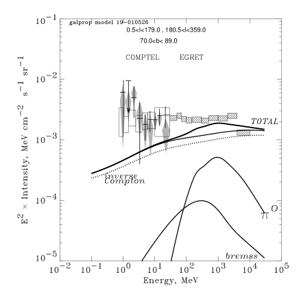
Figure 7.— Gamma-ray energy spectrum of the inner Galaxy (left panel) and from high Galactic latitudes ($|b|\geq 70^{\circ}$, all longitudes) (right panel) as compared with calculations in the HELH model. Separate components show the contribution of bremsstrahlung, $\pi^{0}$-decay, and ICS with (solid line) and without (dotted line) the anisotropic effect. Data in the left panel: EGRET (Strong & Mattox (1996)), COMPTEL (Strong et al.  (1999)), and OSSE (Kinzer, Purcell, & Kurfess (1999)). Data in the right panel: COMPTEL high-latitude total intensity (open boxes: Bloemen et al.  (1999), diamonds: Kappadath (1998), crosses: Weidenspointner et al.  (1999)), and total from EGRET measurements (SMR (99)).

             

Figure 8.— Electron spectra at $R_{s}=8.5$ kpc in the plane, for ‘conventional’ (solid line) and hard electron spectrum (dashes) models. Data points: direct measurements, see references in MS98a .

Figure 9.— The latitude 30–50 MeV $\gamma$-ray profile of the Galaxy as calculated in the HELH model (heavy line; convolved) compared to EGRET data (dots; point sources removed). Separate components show the contribution of bremsstrahlung (thin histogram), $\pi^{0}$-decay (thick histogram), and ICS with (dashes) and without (dash-dots) anisotropic effect; horizontal line: isotropic background.

Fig. 7 shows the spectra of the inner Galaxy ($|b|\leq 5^{\circ}$, $330^{\circ}\leq l\leq 30^{\circ}$) and for high Galactic latitudes ($|b|\geq 70^{\circ}$, all longitudes) as calculated for the HELH model. The HELH model (‘hard electron spectrum and a large halo’, SMR (99)) is chosen to fit high-energy $\gamma$-rays using hard electron spectrum (the injection spectral index is taken as –1.8, with reacceleration) and a broken nucleon spectrum (injection spectral index is –1.8/–2.5 with break at 20 GeV/nucleon, with reacceleration). Such a nucleon spectrum satisfies the limits imposed by antiprotons and positrons (MSR (98), SMR (99)). The halo size taken, $z_{h}=10$ kpc, is within the limits (4–12 kpc) obtained from our ¹⁰Be studies (SM (98)). Following Pohl & Esposito (1998), the consistency with the locally measured electron spectrum above 10 GeV is not required, since the rapid energy losses cause a clumpy distribution so that this is not necessarily representative of the interstellar average. For this case, the interstellar electron spectrum deviates strongly from that locally measured as illustrated in Fig. 9. Because of the increased ICS contribution at high energies, the predicted $\gamma$-ray spectrum can reproduce the overall intensity of the inner Galaxy from 30 MeV to 10 GeV. If the hypothesis of a hard electron injection spectrum is correct in explaining the large-scale Galactic emission, then the same model for the electrons is applicable to the halo where large-scale propagation is relevant. We consider a wide high-latitude region $70^{\circ}<b<90^{\circ}$ which encloses a large volume of halo emission and is therefore unaffected by short-scale fluctuations.

For comparison the dotted lines in Fig. 7 show the spectra of ICS $\gamma$-rays as calculated using the isotropic Jones’ formula (eq. [12]). The model with anisotropic ICS component gives somewhat larger fluxes. The effect is larger at high Galactic latitudes, but also significant for the inner Galaxy. For the case of the inner Galaxy the result is not sensitive to the halo size and for smaller halos the plot would be almost the same. At high latitudes, where the ICS is the only important contributor into the Galactic diffuse emission, it provides up to a factor $\sim 1.4$ larger flux compared to isotropic calculations.

Fig. 9 shows the $\gamma$-ray latitude profile of the Galaxy for 30–50 MeV as calculated in the HELH model, again with and without the anisotropic effect, compared to the EGRET data. For this comparison the $\gamma$-ray sky maps computed in our model have been convolved with the EGRET point-spread function; point sources contribution has been removed from the EGRET data (see SMR (99) for details). At high latitudes the model with anisotropic ICS component again provides significantly larger fluxes compared to isotropic calculations. This is particularly important for estimates of the extragalactic background since Galactic ICS and extragalactic contributions may be comparable.

4. Conclusion

The ICS is a major contributor in the diffuse Galactic emission above $\sim 1$ MeV. Since accurate observational data from EGRET is now available it is desirable to compute the ICS including all important effects. We have shown that the anisotropy of the interstellar radiation field has a significant effect on the intensity and angular distribution of $\gamma$-ray radiation, and can increase the high-latitude Galactic $\gamma$-ray flux up to 40%. This effect should be taken into account when calculating the Galactic emission for extragalactic background estimates.

The derivations presented here provide the basis for the treatment of ICS in our companion study of Galactic diffuse continuum emission (SMR (99)).

References

- Bloemen et al. (1999) Bloemen, H., et al. 1999, Astroph. Lett. Comm. (in Proc. 3rd INTEGRAL Workshop ‘The Extreme Universe’), in press
- Cline & Gao (1992) Cline, D. B., & Gao, Y.-T. 1992, A&A, 256, 351
- Gralewicz et al. (1997) Gralewicz, P., et al. 1997, A&A, 318, 925
- Hunter et al. (1997) Hunter, S. D., et al. 1997, ApJ, 481, 205
- Jauch & Rohrlich (1976) Jauch, J., & Rohrlich, F. 1976, The Theory of Photons and Electrons (New York: Springer)
- Jones (1968) Jones, F. C. 1968, Phys. Rev., 167, 1159
- Jungman, Kamionkowski, & Griest (1996) Jungman, G., Kamionkowski, M., & Griest, K. 1996, Phys. Rep., 267, 195
- Kappadath (1998) Kappadath, S. C. 1998, PhD Thesis, University of New Hampshire, USA
- Kinzer, Purcell, & Kurfess (1999) Kinzer, R. L., Purcell, W. R., & Kurfess, J. D. 1999, ApJ, 515, 215
- Mori (1997) Mori, M. 1997, ApJ, 478, 225
- (11) Moskalenko, I. V., & Strong, A. W. 1998a, ApJ, 493, 694 (MS98a)
- (12) Moskalenko, I. V., & Strong, A. W. 1998b, in Proc. 16th European Cosmic Ray Symposium, ed. J. Medina (Alcalá de Henares: Universidad de Alcalá), p.347, astro-ph/9807288 (MS98b)
- MSR (98) Moskalenko, I. V., Strong, A. W., & Reimer, O. 1998, A&A, 338, L75 (MSR98)
- Page & Hawking (1976) Page, D. N., & Hawking, S. W. 1976, ApJ, 206, 1
- Pohl & Esposito (1998) Pohl, M., & Esposito, J. A. 1998, ApJ, 507, 327
- Porter & Protheroe (1997) Porter, T. A., & Protheroe, R. J. 1997, J. Phys. G: Nucl. Part. Phys., 23, 1765
- Sreekumar et al. (1998) Sreekumar, P., et al. 1998, ApJ, 494, 523
- Strong (1996) Strong, A. W. 1996, Spa. Sci. Rev., 76, 205
- Strong & Mattox (1996) Strong, A. W., & Mattox, J. R. 1996, A&A, 308, L21
- SM (97) Strong, A. W., & Moskalenko, I. V. 1997, in AIP Conf. Proc. 410, Fourth Compton Symposium, ed. C. D. Dermer, M. S. Strickman, & J. D. Kurfess (New York: AIP), p.1162 (SM97)
- SM (98) Strong, A. W., & Moskalenko, I. V. 1998, ApJ, 509, 212 (SM98)
- SMR (99) Strong, A. W., Moskalenko, I. V., & Reimer, O. 1999, ApJ, submitted, astro-ph/9811296 (SMR99)
- Strong et al. (1999) Strong, A. W., et al. 1999, Astroph. Lett. Comm. (in Proc. 3rd INTEGRAL Workshop ‘The Extreme Universe’), in press, astro-ph/9811211
- Weaver (1976) Weaver, T. A. 1976, Phys. Rev. A, 13, 1563
- Weidenspointner et al. (1999) Weidenspointner, G., et al. 1999, Astroph. Lett. Comm. (in Proc. 3rd INTEGRAL Workshop ‘The Extreme Universe’), in press
- Worrall & Strong (1977) Worrall, D. M., & Strong, A. W. 1977, A&A, 57, 229