Spherical Bondi Accretion onto a Magnetic Dipole

Abstract

Quasi–spherical supersonic (Bondi–type) accretion to a star with a dipole magnetic field is investigated using resistive magnetohydrodynamic simulations. A systematic study is made of accretion to a non–rotating star, while sample results for a rotating star are also presented. We find that an approximately spherical shock wave forms around the dipole with an essential part of the star’s initial magnetic flux compressed inside the shock wave. A new stationary subsonic accretion flow is established inside the shock wave with a steady rate of accretion to the star smaller than the Bondi accretion rate $\dot{M}_{B}$. Matter accumulates between the star and the shock wave with the result that the shock wave expands. Accretion to the dipole is almost spherically symmetric at radii larger than $2R_{A}$, where $R_{A}$ is the Alfvén radius, but it is strongly anisotropic at distances comparable to the Alfvén radius and smaller. At these small distances matter flows along the magnetic field lines and accretes to the poles of the star along polar columns. The accretion flow becomes supersonic in the region of the polar columns. In a test case with an unmagnetized star, we observed spherically–symmetric stationary Bondi accretion without a shock wave. The accretion rate to the dipole $\dot{M}_{dip}$ is found to depend on $\beta\propto\dot{M}_{B}/{\hbox{\tenbg\char 22\relax}}^{2}$, where ¯ is the star’s magnetic moment, and $\eta_{m}$ the magnetic diffusivity. Specifically, $\dot{M}_{dip}\propto\beta^{0.5}$ and $\dot{M}_{dip}\propto\eta_{m}^{0.38}$. The equatorial Alfvén radius is found to depend on $\beta$ as $R_{A}\propto\beta^{-0.3}$ which is close to theoretical dependence $\propto\beta^{-2/7}$. There is a weak dependence on magnetic diffusivity, $R_{A}\propto\eta_{m}^{0.07}$.

Simulations of accretion to a rotating star with an aligned dipole magnetic field show that for slow rotation the accretion flow is similar to that in non–rotating case with somewhat smaller values of $\dot{M}_{dip}$. In the case of fast rotation the structure of the subsonic accretion flow is fundamentally different and includes a region of “propeller” outflow. The methods and results described here are of general interest and can be applied to systems where matter accretes with low angular momentum.

Keldysh Institute of Applied Mathematics, Russian Academy of Sciences, Moscow, Russia;
toropin@spp.keldysh.ru

Space Research Institute, Russian Academy of Sciences, Moscow, Russia;
toropina@mx.iki.rssi.ru

Keldysh Institute of Applied Mathematics, Russian Academy of Sciences, Moscow, Russia;

Space Research Institute, Russian Academy of Sciences, Moscow, Russia; and
Department of Astronomy, Cornell University, Ithaca, NY 14853-6801; romanova@astrosun.tn.cornell.edu

Keldysh Institute of Applied Mathematics, Russian Academy of Sciences, Moscow, Russia;
chech@int.keldysh.ru

Department of Astronomy, Cornell University, Ithaca, NY 14853-6801; rvl1@cornell.edu

Accepted to the Astrophysical Journal

Subject headings: accretion, dipole — plasmas — magnetic fields — stars: magnetic fields — X-rays: stars

1 Introduction

Accretion of matter to a rotating star with a dipole magnetic field is a complex and still unsolved problem in astrophysics. The simplest limit is that of accretion to a star with an aligned dipole magnetic field. Although in many cases accretion occurs through a disk, in other cases, where accreting matter has small angular momentum the accretion flow is quasi–spherical at large distances from the star. Examples include some types of wind fed pulsars (see review by Nagase 1989). Also, quasi–spherical accretion may occur to an isolated star if its velocity through the interstellar medium is small compared with the sound speed. Advection dominated accretion ( Paczyński & Bisnovatyi-Kogan 1981; Narayan & Yi 1995) is also expected to be quasi–spherical.

A general analytic solution for spherical accretion to a non–magnetized star was obtained by Bondi (1952). His results have also been confirmed now by numerical three-dimensional (3D) hydrodynamic simulations by Ruffert (1994). The theory and simulations show that matter accretes steadily to the gravitating center without formation of shocks. Accretion of matter with low angular momentum to non-magnetized center was investigated recently by Bisnovatyi-Kogan & Pogorelov (1997). Less attention has been given to quasi–spherical accretion to a magnetized star. Disk accretion to a rotating star with an aligned dipole magnetic field has been investigated in a number of papers both analytically (Pringle & Rees 1972; Ghosh & Lamb 1978; Wang 1979; Shu et al. 1988; Lovelace, Romanova, & Bisnovatyi-Kogan 1995, 1998; Li & Wickramasinghe 1997) and by numerical simulations (Hayashi, Shibata, & Matsumoto 1996; Goodson, Winglee, & Böhm 1997; Miller & Stone 1997).

Investigation of quasi–spherical accretion to a rotating star with dipole field is important because it is a relatively simple limit where different aspects of accretion to a dipole can be observed and clarified. The general nature of quasi–spherical accretion was proposed earlier (Davidson & Ostriker 1973; Lamb, Pethick, & Pines 1973; Arons & Lea 1976; Lipunov 1992, and references therein), but the theoretical ideas have not been tested by MHD simulations. The questions of interest include the global nature of the accretion flow, the location and the shape of the Alfvén surface, and the flow structure, in particular, the departures of the flow from spherical inflow to highly anisotropic polar column accretion inside the dipole’s magnetosphere. Also, it is of interest to verify dependence of the Alfvén radius on the accretion rate, the star’s magnetic moment and rotation rate, and the magnetic diffusivity (considered by Lovelace et al. 1995 for the case of disk accretion).

This paper investigates spherical accretion to a rotating star with an aligned dipole magnetic field by axisymmetric, time–dependent, resistive MHD simulations. Section $2$ describes the model, the equations, the boundary and initial conditions, and the numerical methods used. Section $3$ discusses the results of simulations for non–rotating and rotating central object. A numerical astrophysical example is given in §$3.5$. Section $4$ gives the conclusions of this work.

2 Model

Here, we describe the approach we have taken in axisymmetric MHD simulations of accretion to a rotating star with an aligned dipole magnetic field. We present the mathematical model, including the complete system of resistive MHD equations, the method used to establish the star’s intrinsic dipole magnetic field, the initial and boundary conditions, and a description of the numerical method used to solve the MHD equations.

2.1 System of Equations

We consider the equation system for resistive MHD (Landau & Lifshitz 1960),

$${\partial\rho\over\partial t}+{\bf\nabla}{\bf\cdot}\left(\rho~{}{\bf v}\right)=0{~{},}$$ (1)

$$\rho\left(\frac{\partial{\bf v}}{\partial t}+\left({\bf v}{\bf\cdot}{\bf\nabla}\right){\bf\cdot}{\bf v}\right)=-{\bf\nabla}p+\frac{\left({\bf J\times H}\right)}{c}+{\bf F}^{g}{,}$$ (2)

$$\frac{\partial{\bf H}}{\partial t}={\bf\nabla}{\bf\times}\left({\bf v}{\bf\times}{\bf H}\right)+\frac{c^{2}}{4\pi\sigma}\nabla^{2}{\bf H}{~{},}$$ (3)

$$\frac{\partial(\rho\varepsilon)}{\partial t}+{\bf\nabla}\cdot\left(\rho\varepsilon{\bf v}\right)=-p\left(\nabla{\bf\cdot}{\bf v}\right)+\frac{{\bf J}^{2}}{\sigma}{~{}.}$$ (4)

All variables have their usual meanings. The equation of state is considered to be that for an ideal gas, $p=\left(\gamma-1\right)\rho\varepsilon$, with $\gamma$ the usual specific heat ratio. The equations incorporate Ohm’s law ${\bf J}=\sigma({\bf E}+{\bf v}\times{\bf H}/c)$, where $\sigma$ is the electrical conductivity. In equation (2) the gravitational force ${\bf F}^{g}({\bf R})=-GM\rho{\bf R}/R^{3}$, is due to the central star, where ${\bf R}$ is the radius vector, and $M$ is the star’s mass.

We use an inertial cylindrical coordinate system $\left(r,\phi,z\right)$. The $z$–axis is parallel to the star’s rotation axis and dipole magnetic moment ¯. The coordinate system origin coincides with the star’s center and dipole’s center. Axisymmetry is assumed, ${\partial}/{\partial\phi}=0$. Further, symmetry about the $z=0$ plane is assumed. Thus calculations may be performed on one-quarter of the $r-z$ plane so that the “computational region” is $0\leq R\leq{R}_{max}$, $0\leq z\leq{Z}_{max}$. A totally absorbing sphere, an “accretor” was placed close around the origin. The radius of the accretor was chosen to be small, $r_{accr}\ll R_{max}$.

In order to guarantee that ${\bf\nabla}\cdot{\bf H}=0$ holds for all time in the numerical simulations, we use the vector potential ${\bf A}$ for the magnetic field, ${\bf H}={\bf\nabla}\times{\bf A}$, instead of magnetic field $\bf H$ itself. For axisymmetric conditions equations (1) – (4) can be written in terms of the toroidal vector potential $A_{\phi}$ (or the flux function $\Psi=rA_{\phi}$) and of the toroidal magnetic field $H_{\phi}$:

$$\frac{\partial\rho}{\partial t}+\frac{\partial(\rho v_{z})}{\partial z}+\frac{1}{r}\frac{\partial(r\rho v_{r})}{\partial r}=0{~{},}$$ (5)

$$\frac{\partial(\rho v_{z})}{\partial t}+\frac{\partial}{\partial z}\left(\rho v_{z}^{2}+p+\frac{H_{\phi}^{2}}{8\pi}\right)+\frac{1}{r}\frac{\partial(r\rho v_{z}v_{r})}{\partial r}={}\quad$$

$${}={}-\frac{1}{4\pi}\frac{\partial A_{\phi}}{\partial z}\left(\nabla^{2}A_{\phi}-\frac{A_{\phi}}{r^{2}}\right)+F^{grav}_{z}{~{},}$$ (6)

$$\frac{\partial(\rho v_{r})}{\partial t}+\frac{\partial(\rho v_{z}v_{r})}{\partial z}+\frac{1}{r}\frac{\partial}{\partial r}\left[r\left(\rho v_{r}^{2}+p+\frac{H_{\phi}^{2}}{8\pi}\right)\right]=\quad$$

$${}=\frac{\rho v_{\phi}^{2}+p-\frac{H_{\phi}^{2}}{8\pi}}{r}-\frac{1}{4\pi{}r}\frac{\partial(rA_{\phi})}{\partial r}\left(\nabla^{2}A_{\phi}-\frac{A_{\phi}}{r^{2}}\right)+F^{g}_{r}{~{},}$$ (7)

$$\frac{\partial M_{\phi}}{\partial t}+\frac{\partial(M_{\phi}v_{z})}{\partial z}+\frac{1}{r}\frac{\partial(rM_{\phi}v_{r})}{\partial r}=\quad\qquad\qquad$$

$$=\frac{1}{4\pi}\left(\frac{\partial(rA_{\phi})}{\partial r}\frac{\partial H_{\phi}}{\partial z}\right.-\left.\frac{\partial A_{\phi}}{\partial z}\frac{\partial(rH_{\phi})}{\partial r}\right){~{},}$$ (8)

$$\frac{\partial A_{\phi}}{\partial t}+v_{z}\frac{\partial A_{\phi}}{\partial z}+v_{r}\frac{1}{r}\frac{\partial(rA_{\phi})}{\partial r}=\eta_{m}\left(\nabla^{2}A_{\phi}-\frac{A_{\phi}}{r^{2}}\right){~{},}$$ (9)

$$\frac{\partial H_{\phi}}{\partial t}+\frac{\partial(v_{z}H_{\phi})}{\partial z}+\frac{\partial(v_{r}H_{\phi})}{\partial r}=\frac{\partial}{\partial z}\left(\frac{v_{\phi}}{r}\frac{\partial(rA_{\phi})}{\partial r}\right)-{}\quad$$

$${}-\frac{\partial}{\partial r}\left(v_{\phi}\frac{\partial A_{\phi}}{\partial z}\right)+\eta_{m}\left(\nabla^{2}H_{\phi}-\frac{H_{\phi}}{r^{2}}\right){~{},}$$ (10)

$$\frac{\partial(\rho\varepsilon)}{\partial t}+\frac{\partial(\rho\varepsilon v_{z})}{\partial z}+\frac{\partial(r\rho\varepsilon v_{r})}{r\partial r}=-p\left(\frac{\partial v_{z}}{\partial z}+\frac{\partial(rv_{r})}{\partial r}\right)+$$

$${}+\frac{\eta_{m}}{4\pi}\left[\left(\frac{1}{r}\frac{\partial(rH_{\phi})}{\partial r}\right)^{2}+\left(\frac{\partial H_{\phi}}{\partial z}\right)^{2}+\left(\nabla^{2}A_{\phi}-\frac{A_{\phi}}{r^{2}}\right)^{2}\right]{~{}.}$$ (11)

Here, we have introduced the magnetic diffusivity $\eta_{m}\equiv c^{2}/(4\pi\sigma)={\rm const}$, and $M_{\phi}\equiv\rho v_{\phi}r$, which is the angular momentum density. The poloidal components of the magnetic field are $H_{r}=-{\partial A_{\phi}}/{\partial z}$ and $H_{z}=(1/r){\partial(rA_{\phi})}/{\partial r}$.

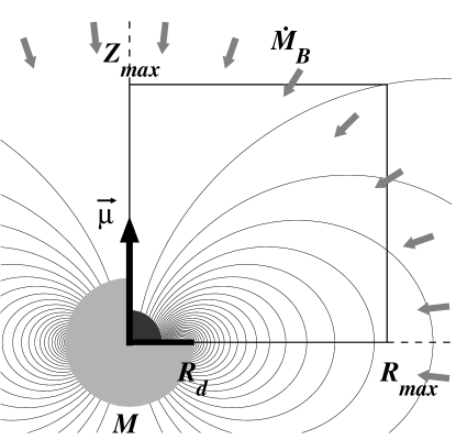
  Fig. 1.—: The figure shows the geometry of the model. A rotating star of mass $M$ and radius $R$ is replaced by infinitesimely thin, rotating, “superconducting” disk $(0<r<R_{d},z=0)$ which is a part of the boundary condition. A fixed azimuthal current flows in this disk and generates the intrinsic dipole-like magnetic field of the star. An absorbing sphere, or “an accretor” with radius $R_{acc}=0.5R_{d}$ is located at the center. We assume axisymmetry and reflection symmetry about equatorial plane. Thus calculations need to be performed only in one quarter of the $(r,z)$ plane, in the box $(0\leq r\leq R_{max},0\leq z\leq Z_{max})$. A spherically symmetric supersonic infow of matter occurs through the outer boundaries of the computational region. The inflow rate is Bondi rate $\dot{M}_{B}$ as discussed in the text.

2.2 Method of Establishing Star’s Dipole Field

The intrinsic magnetic field of the star is generated by current–density ${\bf J}$ flowing inside it. In the absence of plasma currents outside of the star, the vector potential at a point $\bf R$ is ${\bf A\left({\bf R}\right)}=(1/c)\int d^{3}x^{\prime}~{}{\bf J({\bf R^{\prime}})}/|{\bf R}-{\bf R^{\prime}}|$. At large distances from the star, the vector potential can be approximated as ${\bf A}={{{\hbox{\tenbg\char 22\relax}}}\times{\bf R}}/{R^{3}}$, where ${{\hbox{\tenbg\char 22\relax}}}\equiv(1/c)\int d^{3}x~{}{\bf R}\times{\bf J}$ is the intrinsic magnetic moment of the star. The corresponding magnetic field is ${\bf H}=[3{\bf r}\left({{\hbox{\tenbg\char 22\relax}}}\cdot{\bf r}\right)-r^{2}|{{\hbox{\tenbg\char 22\relax}}}|]/{r^{5}}$, which is a “pure” dipole field.

In order to establish an intrinsic stellar dipole field in our simulations we introduce an “external” surface current flowing on a finite part of the equatorial plane, that is, in a disk in the region $0<R_{d}<<R_{max}$. This current models the current flowing inside the star. There are no additional external currents in our model. The presence of this “current disk” creates a dipole–type intrinsic magnetic field in our computational box. The nature of this field is shown in Figure 1.

We choose the azimuthal current–density of the “current disk” to be

$$j_{\phi}\left(r\right)=\int dzJ_{\phi}(r,z)=J_{0}\left(\frac{r}{R_{d}}\right)^{j_{1}}\left(1-\frac{r}{R_{d}}\right)^{j_{2}}~{},$$ (12)

for $0\leq r\leq R_{d}\ll R_{max}$ and $z=0$, where $j_{1}$ and $j_{2}$ are constants. The magnetic moment of this current is

$${{{\hbox{\tenbg\char 22\relax}}}}={\bf e}_{z}\frac{\pi}{c}\int\limits_{0}^{R_{d}}dr^{\prime}{r^{\prime}}^{2}j_{\phi}\left(r^{\prime}\right)~{}.$$ (13)

For the current distribution (12) with $j_{1}=3$ and $j_{2}=1$ (used subsequently in our simulations),

$${{{\hbox{\tenbg\char 22\relax}}}}={\bf e}_{z}{\pi R_{d}^{3}J_{0}\over 42c}{~{}.}$$ (14)

The vector potential corresponding to the azimuthal current density (12) at ${\bf R}=\left(r,z\right)$ is

$$A_{\phi}\left(r,z\right)=\frac{4}{c}\int\limits_{0}^{R_{d}}dr^{\prime}~{}\frac{j_{\phi}\left(r^{\prime}\right)}{k}\sqrt{\frac{r^{\prime}}{r}}\cdot\qquad$$ (15)

$$\qquad\cdot\left[\left(1-\frac{k^{2}}{2}\right)K(k)-E(k)\right]~{},$$

where $k^{2}\equiv 4rr^{\prime}/\left[\left(r+r^{\prime}\right)^{2}+z^{2}\right]$, and $K$, $E$ are the full elliptic integrals of the first and the second type,

$$K(k)\equiv\int\limits_{0}^{\pi/2}d\phi\bigg{/}{\sqrt{1-k^{2}\sin^{2}\phi}}~{},$$

$$E=\int\limits_{0}^{\pi/2}d\phi~{}\sqrt{1-k^{2}\sin^{2}\phi}~{}.$$

We use equations (12) and (15) to numerically determine $A_{\phi}$ in the computational region including the surface of the “current disk”.

The vacuum magnetic field of the “current disk” is given by ${\bf H}={\bf\nabla}\times(A_{\phi}\hat{{\hbox{\tenbg\char 30\relax}}})$ with $A_{\phi}$ given by (15). For example, the magnetic field at the center of the disk for $j_{1}=3$ and $j_{2}=1$ is

$${\bf H}\left(0,0\right)={\bf e}_{z}\frac{\pi J_{0}}{6c}=\frac{7{{{\hbox{\tenbg\char 22\relax}}}}}{R_{d}^{3}}{~{}.}$$ (16)

The magnetic field is found to be close to that of a point dipole for $R>1.5R_{d}$. The initial (vacuum) magnetic field is shown at Figure 1.

2.3 Boundary and Initial Conditions

Here, we consider the boundary conditions on the four sides of our computational region $0\leq r\leq R_{max}$, $0\leq z\leq Z_{max}$ (see Figure 1). We first consider the conditions on the bottom boundary $(0\leq r\leq R_{max},z=0)$. The region of the above mentioned “current disk” ($0\leq r\leq R_{disk}\leq R_{max}$, $z=0$) we treat as perfectly conducting or in effect “superconducting”. We consider the general case where this disk, which represents the star, rotates rigidly with angular rate $\omega$ about the $z-$axis. Consequently, the electric field in the comoving frame of the disk is zero. In the laboratory or non–rotating reference frame, the tangential components of the electric field at ($0\leq r\leq R_{disk}$, $z=0$) are

$$E_{r}(r,0)=-\frac{1}{c}\omega rH_{z}~{},\qquad E_{\phi}(r,0)=0~{}.$$ (17)

These relations hold for all time in our simulations.

Owing to the assumed axisymmetry, ${\bf E}=-(1/c){\partial{\bf A}}/{\partial t}-{\bf\nabla}\Phi=-(1/c)\partial{\bf A}/\partial t$ so that $\partial A_{\phi}/\partial t=-cE_{\phi}$. Consequently, equation (17) gives

$$\frac{\partial A_{\phi}(r,0)}{\partial t}=0\qquad(0\leq r\leq R_{d})~{}.$$ (18)

We also have

$$E_{r}^{disk}=-\frac{\eta_{m}}{c}\frac{\partial H_{\phi}}{\partial z}-\frac{1}{c}\left(v_{\phi}H_{z}-v_{z}H_{\phi}\right)~{},$$

or, using equation (17),

$$\left(v_{\phi}-\omega r\right)H_{z}(r,0)=\eta_{m}\frac{\partial H_{\phi}}{\partial z}\qquad\left(0\leq r\leq R_{d}\right).$$ (19)

For simplicity we consider that the radial current density is zero at the disk for $0\leq r\leq R_{disk}$, $J_{r}=-[{c}/({4\pi})]{\partial H_{\phi}}/{\partial z}=0$. From this we obtain the condition $v_{\phi}=\omega r$ on the current disk part of the $z=0$ boundary. In effect we have a no slip condition on the current disk. The full set of boundary conditions on the current disk $\left(0\leq r\leq R_{d},z=0\right)$ are

$$\quad v_{z}(r,0)=0~{},\quad v_{r}(r,0)=0~{},\quad v_{\phi}(r,0)=\omega r~{},$$

$$\frac{\partial A_{\phi}\left(r,0\right)}{\partial t}=0~{},\quad\frac{\partial H_{\phi}(r,0)}{\partial z}=0~{}.\qquad$$ (20)

The condition $\left.{\partial A_{\phi}\left(r,0\right)}\right/{\partial t}=0$ implies that the vector potential at the surface of the current disk is independent of time. The potential $A_{\phi}\left(r,0\right)$ on this surface is obtained at the beginning of the simulation using equation (15), and it is fixed during the simulation.

The region of the equatorial plane outside of the current disk $\left(R_{d}<r\leq R_{max},z=0\right)$ is treated as a symmetry plane. Thus in this region the boundary conditions are

$$\frac{\partial A_{\phi}(r,0)}{\partial z}=0~{},\quad H_{\phi}(r,0)=0~{},\quad v_{z}(r,0)=0~{}.$$ (21)

Owing to the assumed axisymmetry, the boundary conditions on the $z$-axis $\left(r=0\,,\,0\leq z\leq Z_{max}\right)$ are

$$v_{r}(0,z)=0~{},\quad v_{\phi}(0,z)=0~{},$$

$$A_{\phi}(0,z)=0~{},\quad H_{\phi}(0,z)=0~{}.$$ (22)

Next, we consider the conditions at the outer boundaries. For these boundaries we assume spherically symmetrical inflow with physical values given by the classical Bondi (1952) solution (see also Holzer & Axford 1970). The accretion rate

$$\dot{M}=4\pi\lambda\left(\frac{GM}{c_{\infty}^{2}}\right)^{2}\rho_{\infty}c_{\infty}$$ (23)

in the Bondi solution is defined by the density $\rho_{\infty}$ and the sound speed $c_{\infty}$ at infinity and by the mass of the central object $M$. The characteristic length–scale of the problem is the Bondi radius $R_{B}\equiv{GM}/{c_{\infty}^{2}}$. The type of solution is defined by the value of the dimensionless parameter $\lambda$. The maximum possible value of $\lambda$, denoted $\lambda_{c}$, (for example, $\lambda_{c}=0.625$ for $\gamma=7/5$), corresponds to a flow which is subsonic at infinity and supersonic within the sonic point at a radius $r_{s}=[(5-3\gamma)/{4}]R_{B}$. We used the maximum $\lambda$ Bondi solution for given parameters at infinity for establishing the conditions at the inflow boundaries $\left(r=R_{max},\,0\leq z\leq Z_{max}\right)$ and $\left(0\leq r\leq R_{max},\,z=Z_{max}\right)$. The maximum accretion rate referred to as $\dot{M}_{B}$ correponds to the maximum $\lambda$. Because the inflow is supersonic, all gas dynamical variables can be fixed at the outer boundary.

At the outer inflow boundaries, the magnetic field is assumed to vanish, $H_{\phi}=0$, $A_{\phi}=0$. This is reasonable for situations where the inflowing plasma is unmagnetized. Such an inflow will tend to “carry” inward the dipole field of the star which is relatively weak at the outer boundaries. However, for comparison we tested different conditions for non-zero $A_{\phi}$ on the outer boundaries, for example, ${\partial A_{\phi}}/{\partial{\bf n}}=0$. Our numerical results show no dependence of the flow on the outer conditions on $A_{\phi}$.

An absorbing sphere or an “accretor” is located close around the origin $(r,z)=0$. It prevents matter accumulation in the region close to the gravitating center. The radius of the accretor is taken to be $R_{accr}=0.5R_{d}$ (see Figure 1). After each time step, the matter pressure inside this sphere is set to a small value in comparison with the pressure in the immediately surrounding region. The typical pressure contrast was $1/1000$. This allows the matter just outside the “accretor” to expand freely inward into the low pressure region $R\leq R_{accr}$. Thus, super slowmagnetosonic inflow into the accretor is realized during the simulations. In contrast to pure hydrodynamic simulations (for example, Ruffert 1994), the density is not small inside the “accretor”. Close to the origin, the magnetic field has its highest value. A low density in this region gives a high Alfvén speed and therefore a very small time step as follows from the Courant–Friedrichs–Levy condition. For this reason the density inside the “accretor” was set equal to a fraction of the exterior density while the temperature was set to a small fraction of the exterior temperature in order to provide the mentioned pressure contrast with the matter just outside the accretor.

At $t=0$, magnetic field is obtained from the vacuum vector potential $A_{\phi}$ of equation (15). For all runs, with non-rotating and rotating central objects, the azimuthal magnetic field is zero, $H_{\phi}({\bf r},t=0)=0$. Density, pressure, and velocity fields were taken from the Bondi solution with maximum possible accretion rate. Inside a sphere with radius $R=3R_{d}$, the velocity at $t=0$ was set to zero.

2.4 Dimensionless Parameters and Variables

It is helpful to put equations (5)–(11) into dimensionless form. For this we use the values $\rho_{\infty}$, $H_{0}$, and $R_{d}$ for the density, the magnetic field, and the length, respectively, where $\rho_{\infty}$ is the density at the infinity, $H_{0}=H_{z}\left(0,0\right)$ is the magnetic field at the center of our smoothed dipole field (equation 16), and $R_{d}$ is the radius of the current disk (equation 12). For the simulations presented here, the ratio of $R_{d}$ to the Bondi radius $R_{B}\equiv GM/c_{\infty}^{2}$ was chosen to be

$${R_{d}\over R_{B}}=\frac{1}{50\sqrt{2}}{~{}.}$$ (24)

Note that for $\gamma=7/5$, the sonic radius of the Bondi flow is at $r_{s}=[(5-3\gamma)/4]R_{B}=10\sqrt{2}R_{d}$.

The values

$$V_{A0}\equiv{H_{0}\over\sqrt{4\pi\rho_{\infty}}}~{},\qquad p_{0}={H_{0}^{2}\over 8\pi}$$ (25)

provide units for the velocity and pressure. After reducing the equations (5)–(11) to dimensionless form, a non–standard plasma parameter,

$$\beta\equiv\frac{8{\pi}P_{\infty}}{{H_{0}}^{2}}=\frac{2}{\gamma}\frac{c_{\infty}^{2}}{V_{A0}^{2}}~{},$$ (26)

appears. This is the ratio of the plasma pressure at infinity to the magnetic pressure near the origin. This parameter connects the two parts of the considered problem, the gas dynamical unperturbed Bondi flow at large distances with the stellar dipole magnetic field at small distances.

The Alfvén radius $R_{A}$ for quasi–spherical accretion onto a magnetic dipole is given roughly by the balance of ram pressure of the flow $\rho v^{2}_{ff}\sim\dot{M}v_{ff}/(4\pi R^{2})$ with the magnetic pressure ${\bf H}^{2}/(8\pi)\sim\mu^{2}/(8\pi R^{6})$, where $v_{ff}=\sqrt{2GM/R}$ is the free–fall speed. Thus we define

$$R_{A}^{th}\equiv\left(\frac{\mu^{2}}{2\dot{M}\sqrt{2GM}}\right)^{2/7}{~{}.}$$ (27)

Taking into account that for maximum Bondi accretion rate $\dot{M}=\dot{M}_{B}=4\pi\lambda_{c}R_{B}^{2}\rho_{\infty}c_{\infty}$, we have

$${R_{A}^{th}\over R_{d}}=k~{}\beta^{-{2/7}}~{},\quad{\rm where~{}~{}~{}}k\equiv{(R_{d}/R_{B})^{5/7}\over(49\sqrt{2}\gamma\lambda_{c})^{2/7}}~{}.$$ (28)

Thus, our $\beta$ parameter from equation (26) determines the ratio of the Alfvén radius (27) to the current disk radius. The dependence $R_{A}^{th}\propto\beta^{-2/7}$ for $R_{d}/R_{B}$ fixed shows that $\beta\propto\dot{M}_{B}/\mu^{2}$. The important quantity $\dot{M}_{B}/\mu^{2}$ is referred to as the “gravimagnetic” parameter by Davies & Pringle (1981) (see also Lipunov 1992). Equation (28) for the Alfvén radius as a function of $\beta$ is discussed further in § 3.3.

Another important dimensionless parameter of the model is the magnetic Reynolds number,

$$Re_{m}\equiv{R_{0}V_{0}\over\eta_{m}}={4\pi\sigma R_{0}V_{0}\over c^{2}}~{},$$ (29)

where $\eta_{m}$ is the magnetic diffusivity, $R_{0}$ is a characteristic scale and $V_{0}$ is a characteristic speed of the accretion flow. The value of the magnetic Reynolds number $Re_{m}$ depends on the chosen length scale $R_{0}$. Here, it is appropriate to evaluate $Re_{m}$ at the Alfvén radius where $R_{0}V_{0}\approx\sqrt{2GMR_{A}}$. Thus it is useful to introduce the dimensionless magnetic diffusivity,

$$\tilde{\eta}_{m}\equiv{\eta_{m}\over R_{A}V_{A}}={1\over Re_{m}}{~{}.}$$ (30)

Numerical values are discussed in § 3.4.

We do not offer a detailed explanation for the magnetic diffusivity $\eta_{m}$. However it could arise from three–dimensional MHD instabilities not accounted for in our two–dimensional (axisymmetric) simulations. An important instability is the interchange or Rayleigh–Taylor instability with wavevector in the azimuthal direction ${\bf k}=k_{\phi}\hat{\phi}$ (Arons & Lea 1976; Elsner & Lamb 1977). This instability allows blobs or filaments of plasma to fall inward across the magnetic field. Of course, perturbations with $k_{\phi}\neq 0$ are not allowed in the present axi–symmetric simulations.

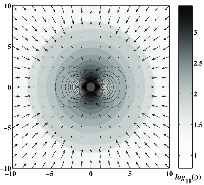
  Fig. 2.—: The figure shows an example of our calculated flow for accretion onto a non-rotating star with a dipole magnetic field at $t=2.5t_{ff}$. The run is characterized by the dimensionless parameters $\beta=3.5\times 10^{-7}\propto\dot{M}_{B}/{\hbox{\tenbg\char 22\relax}}^{2}$ and magnetic diffusivity $\tilde{\eta}_{m}=10^{-5}$, where $\dot{M}_{B}$ is the accretion rate and ¯ is the star’s magnetic moment. The background gray scale represents the density of the flow and the solid lines the poloidal magnetic field lines. The length of the arrows (shown at every 32^th cell along both directions) is proportional to flow speed. The internal circular region represents the “accretor.” The shock wave and associated transition from supersonic to subsonic flow is evident. The flow becomes strongly anisotropic close to the dipole. The simulations were done on a grid of $257\times 257$ cells in one quadrant of the physical space. Only one quadrant is needed due to the assumed axisymmetry and the symmetry about the equatorial plane.

2.5 Numerical Method

Finite difference methods are used to solve the axisymmetric MHD equations (5) – (11). The calculations are done in five main stages:

In the first stage, equations (9) and (10) for the fields $A_{\phi}$ and $H_{\phi}$ are solved with the right–hand sides of the equations set equal to zero. That is, we first solve for the advection of these fields. For this stage, we use the hybrid numerical scheme proposed by Kamenetskyi & Semyonov (1989). This is based on two well known methods, the Lax – Wendroff method for the region where the solution is “smooth”, and a numerical scheme with differences against the flow for the “non–smooth” regions.

For the second stage, the finite conductivity is taken into account in the equations for $A_{\phi}$ and $H_{\phi}$ with the advection terms omitted. That is, we now solve parabolic equations for these fields. For this, an explicit multistage numerical scheme is used. This scheme is called the “Method of Local Iterations” (MLI), and it is described in detail by Zhukov, Zabrodin, & Feodoritova (1993). The MLI scheme is explicit and absolutely stable.

For the third stage, we solve the equations (5) – (11) including the magnetic terms but omitting the advection terms. At this stage the magnetic terms are known.

For the fourth stage the full advection equations for $\rho$, $\rho{\bf v}$, and $\rho\epsilon$ are solved. For this we use an adaptation of Flux Corrected Transport method (FCT), based on ideas discussed by Boris & Book (1973). The transport of each density, for example, $\rho$, to the next time level is realized in several stages. In one of the stages explicit correction of the fluxes is done. The procedure is performed separately along the $r$ and $z$ coordinates using a dimensional split technique (Strang 1968).

In the fifth and final stage, the Joule heating is taken into account in equation (11) for the internal energy. Overall, our finite difference method is second order accurate in space and time for smooth flows. This method and numerical scheme was tested widely and also was successfully used earlier (Savelyev and Chechetkin 1994; Savelyev et al. 1996, Toropin et al. 1997).

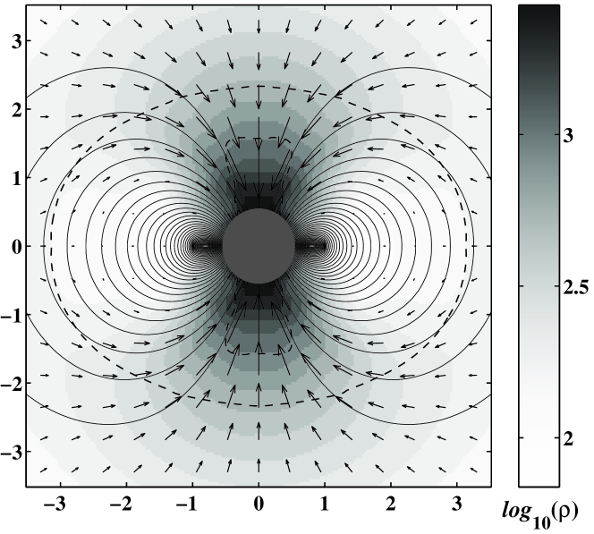
  Fig. 3.—: Enlarged view of the inner region of the plot of Figure 2. The anisotropy of the flow is evident. The torus–like region with small flow velocities is the “stagnation zone”. In the equatorial plane, the outer boundary of this zone is the magnetopause with radius $R_{mp}\approx 2.6{}R_{d}$. There are two ($\pm~{}z$) polar accretion columns. The outer dashed line represents the Alfvén surface. At very small distance from the star, the flow in the polar columns becomes supersonic. The sonic surface is marked by a dashed line in the region of polar columns.

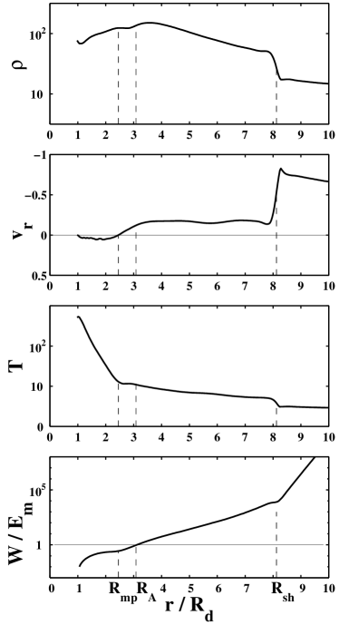
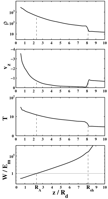
  Fig. 4.—: The figure shows the radial variation of density $\rho$, radial velocity $v_{r}$, temperature $T$, and ratio of total kinetic energy-density of the matter $W=\rho(\varepsilon+{\bf v}^{2}/2)$ to the magnetic energy–density $E_{m}={\bf H}^{2}/8\pi$ in the equatorial plane (left column) for the acccretion flow presented at Figure 2 $(t=3.5t_{ff})$. The positions of the Alfvén radius $r=R_{A}$, the magnetopause $r=R_{mp}$ and the shock wave $r=R_{sh}$ are shown. Right columns show the $z-$dependences of the same parameters along the $z-$axis. The positions of the shock wave $z=R_{sh}$ and Alfvén radius $z=R_{A}$ are shown.

3 Results

This work investigates spherical Bondi–type accretion of plasma to a star with an aligned dipole magnetic field. The resistive MHD equations (5) – (11) were solved using the method described in §2.5 and initial and boundary conditions described in §2.2 and §2.3.

We performed simulations for $12$ different values of $\beta\propto\dot{M}_{B}/{\hbox{\tenbg\char 22\relax}}^{2}$ (equation 26), and magnetic diffusivities $\tilde{\eta}_{m}$ (equation 30). The calculated flows in all runs are similar to that shown in Figure 2. In § 3.1, we describe in detail the nature of the flow for a representative run. In § 3.2 we analyze the stationarity of the spherical accretion to a dipole. In § 3.3, we show the dependence of the flows on $\beta$ and $\tilde{\eta}_{m}$. In § 3.4, sample runs of accretion to a rotating star are presented. In § 3.5, we give a numerical application of our results.

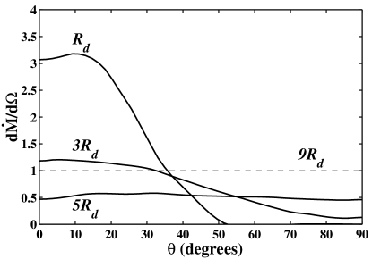
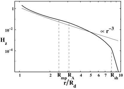
  Fig. 5.—: Differential mass accretion rate per unit solid angle $d\dot{M}/d\Omega$ as a function of the angle $\theta$ (with respect to the $z-$axis) for spheres with radii $R_{d}$, $3R_{d}$, $5R_{d}$, and $9R_{d}$ for the flow presented in Figure 2. At large distances ($R=5R_{d}$) accretion is almost spherically symmetric. Closer to the dipole ($R=3R_{d}$), the flow becomes anisotropic. At very small distances ($R=R_{d}$) most of the matter accretes to the poles along a narrow cone of half–angle $\theta_{1/2}\approx 30^{\circ}$.

  Fig. 6.—: Radial variation of the vertical magnetic field $H_{z}$ in the equatorial plane. The thin line shows the dependence of $H_{z}$ for a vacuum dipole field. The vertical dashed lines indicate the positions of the shock wave $R_{sh}$, Alfvén radius $R_{A}$, and magnetopause radius $R_{mp}$.

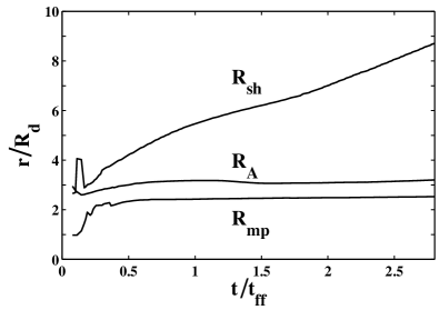
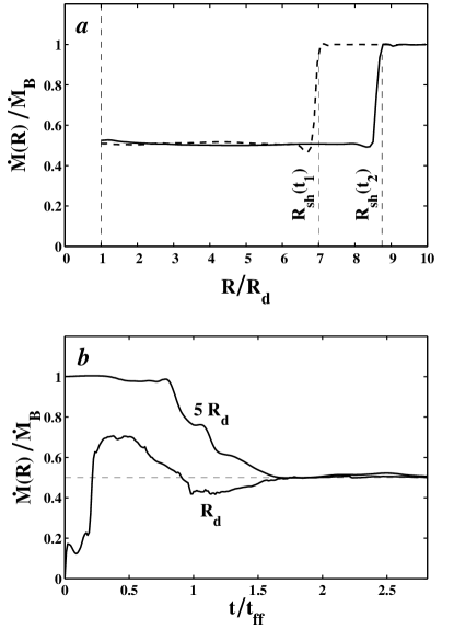
  Fig. 7.—: Temporal evolution of the shock wave radius $R_{sh}$, Alfvén radius $R_{A}$, and magnetopause radius $R_{mp}$. Time is measured in units of $t_{ff}$ which is the free–fall time from the distance $R_{max}$.

  Fig. 8.—: (a) Mass accretion rate $\dot{M}$ through spheres of radii $R$ at $t_{1}=2t_{ff}$ (dashed line) and $t_{2}=2.8t_{ff}$ (solid line). The shock wave expands from position $R=R_{sh}(t_{1})$ to position $R_{sh}(t_{2})$. Inside the shock the flow is subsonic with accretion rate $\dot{M}_{dip}\approx{}0.5\dot{M}_{B}$. (b) Time evolution of mass–fluxes $\dot{M}(R)/\dot{M}_{B}$ throught spheres with radii $R=R_{d}$ and $R=5R_{d}$.

3.1 Illustrative Simulation Run

Here we describe in detail a run with $\beta=3.5\times 10^{-7}$ and $\tilde{\eta}_{m}=10^{-5}$. Simulations were performed on a uniform grid with $257{}\times{}257$ square cells. The size of the computational region was $10R_{d}\times{}10R_{d}$, the accretor radius was $0.5R_{d}$, where $R_{d}$ is the radius of the current disk. We measure time in units of the free–fall time from $r=R_{max}$, $z=0$; that is, $t_{ff}=R_{max}^{3/2}/\sqrt{2GM}$.

Spherical accretion to a magnetic dipole is very different from that to a non–magnetized star. Instead of supersonic steady inflow, which is observed in standard Bondi accretion, a shock wave forms around the dipole. The supersonic inflow outside the shock becomes subsonic inside it. In all cases we observe that the shock wave gradually expands outwards. Figure 2 shows the main features of the flow at time $t\approx 2.5t_{ff}$ when the shock has moved to the distance $R_{sh}=8.1R_{d}$. We observe that for $R>R_{sh}$ the flow is unperturbed Bondi flow, whereas inside the shock for $R<R_{sh}$ it is subsonic. Initially, the subsonic accretion to dipole is spherically symmetric, but closer to the dipole it becomes strongly anisotropic. Near the dipole matter moves along the magnetic field lines and accretes to the poles. Figure 3 shows the inner subsonic region of the flow in greater detail. The dashed line shows the Alfvén surface, which we determine as the region where the matter energy–density $W=\rho(\varepsilon+{\bf v}^{2}\!/\!2)$ is equal to the magnetic energy–density $E_{m}={\bf H}^{2}/(8\pi)$. The Alfvén surface is ellipsoidal, with radius $R_{A}=3.1R_{d}$ in the equatorial plane, and $R_{A}=2.3R_{d}$ along the $z-$axis. Note, that the “theoretically” estimated Alfvén radius (28) is $R_{A}^{th}\approx{}2.6R_{d}$. A significant deviation from spherically symmetric flow is observed for $R\mathrel{\hbox{\hbox to0.0pt{\hbox{\lower 4.0pt\hbox{$\sim$}}\hss}\hbox{$<$}}}2R_{A}$, because magnetic field starts to influence the flow before it reaches the Alfvén surface. Matter in the equatorial plane moves across the magnetic field lines, decelerates and stops at a radius $r=R_{mp}\approx 2.6R_{d}$, which we term the “magnetopause radius.” There is a torus shaped region – a stagnation region – which is avoided by accretting matter. The flow velocities in this region are negligible. The magnetopause region is located inside the Alfvén surface (see Figure 3). The accretion flow along the $z-$axis is accelerated and becomes supersonic at $z\approx 1.6R_{d}$ (see inner dashed line at Figure 3).

Figure 4 show the radial and axial variation of different parameters. One can see, that the density $\rho$ is larger in the subsonic region compared with the Bondi solution. The velocity decreases by about a factor of $4$ across the shock wave, and the temperature increases. The density in the magnetopause region $R\leq R_{mp}$ is lower than outside, while the temperature is larger (see Figure 4, left column). The bottom panel of Figure 4 shows the variation of ratio $W/E_{m}$. The radius where $W/E_{m}=1$ is Alfvén radius. In the $z$-direction (see Figure 4, right column), matter moves along the magnetic field lines with the result that the flow parameters change smoothly.

Figure 6 shows the transition from spherically symmetric accretion outside the magnetosphere to highly anisotropic accretion along the polar columns within the magnetosphere. The figure shows the matter flux accreting through the unit solid angle $d\dot{M}/d\Omega$ at different inclinations $\theta$ of this solid angle relative to the $\pm z$ axis. One can see that at large distances $R=5R_{d}$, the accretion is almost spherically symmetric, whereas at smaller distances it becomes more and more anisotropic.

Figure 6 shows that the initial vacuum dipole magnetic field (Figure 1) is strongly compressed by the incoming Bondi flow. As a result of interaction with Bondi flow, the magnetic field has a dipole dependence only inside Alfvén radius, $r\mathrel{\hbox{\hbox to0.0pt{\hbox{\lower 4.0pt\hbox{$\sim$}}\hss}\hbox{$<$}}}R_{A}$, and it decreases faster than the dipole field for $R_{A}\leq r\leq R_{sh}$. This is a result of an induced azimuthal shielding current in the dipole’s magnetosphere. Thus distributed current has a sign opposite to that of the star’s intrinsic azimuthal current. For $r\mathrel{\hbox{\hbox to0.0pt{\hbox{\lower 4.0pt\hbox{$\sim$}}\hss}\hbox{$>$}}}R_{sh}$, the field decreases dramatically with $r$ due to the shielding current. Thus, the magnetic field at the outer boundary of the simulation region is negligible.

Figure 8 shows that the shock wave initially forms close to the magnetosphere at $R\sim R_{A}$ and then gradually expands outward. However, the Alfvén radius $R_{A}$ and magnetopause radius $R_{mp}$ become steady after $t\mathrel{\hbox{\hbox to0.0pt{\hbox{\lower 4.0pt\hbox{$\sim$}}\hss}\hbox{$>$}}}t_{ff}/2$ and remain steady thereafter. This means, that the magnetosphere of the star reaches equilibrium with the incoming matter rapidly and this equilibrium does not change as a result of outward movement of the shock wave.

3.2 Stationarity of Accretion Flow to the Dipole

It is important to know whether the calculated accretion flow to the dipole is stationary or not. We analyze this here.

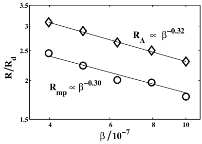
  Fig. 9.—: Dependence of the Alfvén radius $R_{A}$ and magnetopause radius $R_{mp}$ on parameter $\beta\propto\dot{M}_{B}/\mu^{2}$ for magnetic diffusivity $\tilde{\eta}_{m}=10^{-5}$.

After the passage of the shock wave, the new subsonic regime of accretion forms around the dipole. The region of subsonic flow expands together with the expanding shock wave. Here, we analyze the stationarity of the flow in the subsonic region. Figure 8a shows the distribution of matter fluxes through spheres of different radii $\dot{M}(R)$ as a function of $R$ at $t=2t_{ff}$ and $t=2.8t_{ff}$. One can see that matter flux outside the shock wave $R>R_{sh}$ is the Bondi rate $\dot{M}_{B}$, while inside the shock wave it is significantly less. It is almost constant and equal to the accretion rate to the dipole $\dot{M}(R)\approx\dot{M}_{dip}\approx 0.5\dot{M}_{B}$.

Figure 8b shows the matter fluxes through fixed spheres located at radii $R=R_{d}$ and $R=5R_{d}$ as a function of time. The matter flux through the sphere of radius $R=R_{d}$ corresponds to the matter flux to the dipole. It decreases and goes to the constant $\dot{M}=\dot{M}_{dip}$ at $t>1.5t_{ff}$. The matter flux through the sphere $R=5R_{d}$ is initially the Bondi rate, but after passage of the shock wave it decreases to $\dot{M}=\dot{M}_{dip}$ and does not change thereafter. Thus, Figures 8a and 8b demonstrate that the flow in the subsonic region is stationary in both space and time. The shock wave switches the Bondi flow to a new flow with stationary subsonic accretion and smaller accretion rate. The local physical variables, for example, density $\rho$ and velocity ${\bf v}$ are also time independent.

The formation of an expanding shock wave during accretion to a dipole results from the fact that the gravitating center with dipole field “absorbs” matter at a slower rate than the Bondi rate. The rate of accretion $\dot{M}_{dip}$ at given parameters of the Bondi flow is determined by the physical parameters of the dipole (see § 3.3).

An analogous situation was found in investigations of hydrodynamical accretion to a gravitating center. Kazhdan & Lutskii (1977) (see also Sakashita 1974; Sakashita & Yokosawa 1974; Kazhdan & Murzina 1994) investigated spherically symmetric accretion flows for conditions where the matter flux through the inner boundary (which is the surface of the star) is less than matter flux supplied at the outer boundary. They found a family of self–similar solutions where the expanding shock wave links the regions inside and outside the shock wave. These regions have different stationary matter fluxes corresponding to matter fluxes at the boundaries. Our simulations show similar behaviour.

Here, we should point out that the shock wave in our simulations is a temporary phenomenon, which establishes a new regime of accretion around the dipole. It appeared because the external accretion rate is larger than accretion rate which dipole can “absorb.” A different situation was considered by Ruffert (1994) who performed 3D hydrodynamical simulations of Bondi accretion. He used initial conditions where the matter distribution had constant density and zero velocity. In his simulations, the initial matter flux is zero and stationary accretion was established by a rareaction wave propagating outward from the central object.

For fixed boundary conditions (supersonic Bondi accretion at the outer boundary) the results of simulations do not depend on initial conditions. The dependence on boundary conditions will be investigated separately.

It is of interest to know how far outward the the shock wave will propagate. Note that the Bondi flow is supersonic out to some distance and is subsonic at larger distances. We expect that after reaching the subsonic area, the shock wave will “dissolve” and the flow will be purely subsonic. Thus, the shock wave may be only a temporary phenomenon which results from the initial conditions of our simulations. From the other side, if the flow is supersonic up to very large distances, then the shock wave expansion may be stopped by the physical structure of the astrophysical system. For example, in the wind-fed pulsars, the shock movement would stop at a radius of the order of the binary separation.

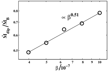
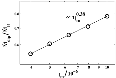
  Fig. 10.—: Dependence of accretion rate to the dipole $\dot{M}_{dip}$, measured in Bondi accretion rate $\dot{M}_{B}$, on $\beta$ (at $\tilde{\eta}_{m}=10^{-5}$, left frame) and on $\tilde{\eta}_{m}$ (at $\beta=10^{-6}$, right frame).

3.3 Dependence of the Accretion Flow on $\beta\propto{\dot{M}_{B}/\mu^{2}}$ and $\tilde{\eta}_{m}$

We first analyze the dependence of the flow on the external accretion rate $\dot{M}_{B}$ and the star’s magnetic moment ¯. As discussed in § 2.4, these quantities are coupled so that the investigated physical model depends only on the ratio $\beta{}\propto{}{\dot{M}_{B}}/{{\hbox{\tenbg\char 22\relax}}^{2}}$. Each simulation run takes considerable time and for this reason we adopted the following procedure for deriving the dependence on $\beta$. We start from the conditions of the simulation run of with $\beta=10^{-6}$ at time $t=2t_{ff}$, and then change $\beta$ by a factor of $10^{n/10}$ in a sequence of $5$ independent simulations ($n=1\ldots 5$). These simulations were performed up to $t=5t_{ff}$. Fluctuations connected with the readjustment of the flow are damped by this time. We then measured the radius of the magnetopause $R_{mp}$ and the Alfven radius $R_{A}$ for new values of $\beta$. The Alfvén radius in the equatorial plane is found to have a power law dependence,

$$R_{A}(\beta)\approx 2.3{}R_{d}\left(\frac{\beta}{10^{-6}}\right)^{-k_{\beta}}{~{},}$$ (31)

where $k_{\beta}\approx 0.32\pm 0.03$ $(\sim 2/7\approx 0.286)$. The equatorial magnetopause radius is found to be proportional to the Alfvén radius, $R_{mp}(\beta)\approx 0.026R_{d}+0.756R_{A}(\beta)$. Figure 9 shows the observed dependences. The Alfvén radius is found to have a weak dependence on magnetic diffusivity $\eta_{m}$, $R_{A}\sim\tilde{\eta}_{m}^{-k_{\eta}}$, where $k_{\eta}\approx 0.075$.

Figure 10 shows that the stationary accretion rate to the dipole ${\dot{M}}_{dip}$ also depends on $\beta$. We find that $\dot{M}_{dip}$ is always smaller than the Bondi accretion rate $\dot{M}_{B}$. The dependence found is

$${\dot{M}}_{dip}\approx 0.78{\dot{M}}_{B}\left(\frac{\beta}{10^{-6}}\right)^{m_{\beta}}{~{},}$$ (32)

for $\beta\leq 10^{-6}$, where $m_{\beta}\approx 0.51$.

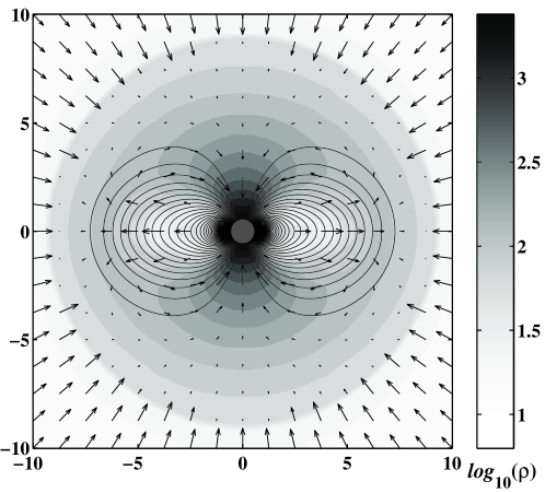
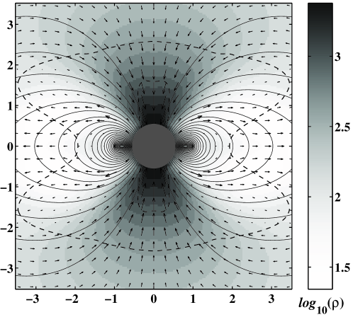
  Fig. 11.—: The figure shows the accretion flow to a rapidly rotating star (see §3.3) at time $t=2.5t_{ff}$ . The gray–scale background represents the density and the solid lines the poloidal magnetic field. The length of arrows is proportional to the flow speed.

  Fig. 12.—: Enlarged view of the accretion flow to a rapidly rotating star with dipole field (Figure 12). The outer dashed line represents the Alfvén surface. A inner sonic surface is indicated by the dashed line in the region of polar columns. The outflow in the equatorial plane starts from the region of the corotation radius $R_{cr}=2{}R_{d}$ inside magnetosphere.

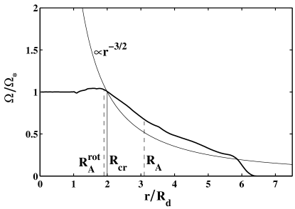
  Fig. 13.—: The radial variation of the angular velocity of the matter $\Omega(r)=v_{\phi}(r)/r$ in the equatorial plane measured in units of angular velocity of the disk $\Omega_{\star}$ (solid line). The thin solid line shows the radial dependence of the Keplerian angular velocity. The positions of the corotation radius $R_{cr}$ and $R_{A}^{rot}$ are shown. Also, the position of the Alfvén radius for the corresponding non–rotating system $R_{A}$ is marked.

Here, we recall that $\beta\propto{}\dot{M}_{B}/{\hbox{\tenbg\char 22\relax}}^{2}$ and in equation (23) for $\dot{M}_{B}$ all quantities except $\rho_{\infty}$ are fixed in our simulations. Thus, the accretion rate to the dipole depends on the density of surrounding matter as $\dot{M}_{dip}\propto\rho_{\infty}^{3/2}$ and on the star’s magnetic moment as $\dot{M}_{dip}\propto{}1/{|{\hbox{\tenbg\char 22\relax}}|}$. The last dependence can be explained by the fact that at larger $\beta$, the Alfvén radius is smaller so that the opening angle of the accretion columns is larger. As a result, matter can more readily flow into the gravitating center. At $\beta>3\cdot{}10^{-6}$, the dependence is different. ${\dot{M}}_{dip}$ increases more gradually and approaches the critical Bondi accretion rate $\dot{M}_{B}$. Here, we observe stationary Bondi flow similar to that observed in simulations to non–magnetized gravitating object (Ruffert 1994).

Figure 10 shows the dependence of the accretion rate on the magnetic diffusivity

$${\dot{M}}_{dip}\approx 0.78{\dot{M}}_{B}\left(\frac{\tilde{\eta}_{m}}{10^{-5}}\right)^{m_{\eta}}{~{},}$$ (33)

for $\tilde{\eta}_{m}\leq 10^{-5}$, $m_{\eta}\approx 0.38$. This dependence means that matter accretes more readily at larger diffusivity as expected.

The half–opening angle $\theta_{1/2}$ of the accretion funnel at $r=R_{d}$ (see Figure 6) decreases as $\tilde{\eta}_{m}$ decreases. We find $\theta_{1/2}\propto{}(\tilde{\eta}_{m})^{0.26}$.

At higher difusivities $\tilde{\eta}_{m}>10^{-5}$, the dependence (33) becomes smoother, $\dot{M}_{dip}\rightarrow\dot{M}_{B}$ and we observe steady accretion at the Bondi rate.

3.4 Accretion to a Rotating Dipole

We also investigated cases of accretion to a rotating star with an aligned dipole magnetic field. To create the rotating dipole, we rigidly rotated the current disk $0\leq r\leq R_{d}$ which is a part of boundary condition at $z=0$ as discussed in §2.3. The disk radius $R_{d}$ is in effect the radius of the star. We discuss two cases, one with slow rotation, $\Omega_{\star}=0.1\Omega_{K}(R_{d})$, and the other with fast rotation, $\Omega_{\star}=0.35\Omega_{K}(R_{d})$, where $\Omega_{\star}$ is the star’s angular rotation rate and $\Omega_{K}(R_{d})=\sqrt{GM/R_{d}^{3}}$ is the Keplerian angular velocity at the edge of the disk $r=R_{d}$.

We observed that in the case of slow rotation the general behavior of accretion flow is similar to that for the non–rotating case. The corotation radius $R_{cr}$, where $\Omega_{K}(R_{cr})=\Omega_{\star}$ or $R_{cr}=(GM/\Omega_{\star}^{2})^{1/3}$, is significantly larger than the Alfvén radius $R_{A}$ for a non-rotating dipole.

As in the non-rotating case, the shock wave forms and propagates outwards, while accretion to the dipole is subsonic and steady. However, a new feature appears: The stagnation region mentioned earlier rotates rigidly with the angular velocity of the star. We find that the limit of slow rotation is valid for $R_{cr}>R_{A}$. In this case the linear velocity of rotation at the outer edge of magnetosphere ($R=R_{A}$) is smaller than the Keplerian velocity. In cases of slow rotation, accretion to the dipole is steady but with an accretion rate $\dot{M}_{dip}^{rot}$ which is smaller than the corresponding value for a non-rotating star, $\dot{M}_{dip}$.

The second case we discuss is a rapidly rotating dipole, where the corotation radius is smaller than the Alfvén radius for the corresponding system with a non–rotating star, $R_{cr}<R_{A}$. In this case the outer equatorial region of the rotating magnetosphere, $R_{cr}<r<R_{A}$, has azimuthal velocities in excess of Keplerian velocity. Matter moves outwards in a wide “belt”– like region around the equatorial plane. Figures 12 and 12 show the simulation results for $\Omega_{\star}=0.35\Omega_{K}$ when the corotation radius is $R_{cr}=2.0R_{d}$, and the Alfvén radius in the equatorial plane is $R_{A}^{rot}=1.9R_{d}$. One can see, that magnetic field lines are elongated in equatorial direction by outflowing matter. The strongest outward acceleration is in the equatorial plane where the centrifugal force is largest. However, in the region of Alfvén surface (see Figure 12), an essential acceleration is observed along the magnetic field lines. This acceleration appears to determine the unusual shape of the Alfvén surface (see Figure 12). Also, an essential outflow may occur above and below the equator.

At larger radial distances, the outflowing matter encounters the incoming Bondi flow and turns to the direction of poles. The magnetic field lines are elongated in the $r$-direction. The Alfvén radius in the direction of the poles has a value similar to that in the non-rotating case. However, in the equatorial plane the Alfvén radius is significantly smaller ($R_{A}^{rot}\approx 1.9R_{d}$) than its non-rotating value ($R_{A}\approx 3.1R_{d}$). Figure 13 shows that the magnetosphere inside $r<R_{A}^{rot}$ rotates rigidly. The angular velocity decreases gradually for $r>R_{A}^{rot}$. The Figure also shows that the angular velocity of matter is larger than Keplerian in the outer parts of the magnetosphere beyond the Alfvén radius. In this region, the centrifugal force expells matter outward forming “propeller” – like outflows. The “propeller” outflows are predicted to occur in the magnetosphere of a rapidly rotating magnetized star as first discussed by Illarionov and Sunyaev (1975). The theory of such outflows has received renewed interest for the case of disk accretion to rotating magnetized stars (Li & Wickramasinghe 1997; Lovelace, Romanova, and Bisnovatyi-Kogan 1998). A systematic study of spherical accretion to a rotating star with an aligned dipole magnetic field is in preparation (Toropin et al. 1998).

3.5 Astrophysical Example

Here, we present an application of our simulation results in terms of the physical quantities. We consider Bondi accretion to a non-rotating magnetized protostar with mass $M=1~{}M_{\hbox{$\odot$}}=2\times 10^{33}$ g and radius $R=10^{11}$ cm. We use our simulation run with $\beta=10^{-6}$ and $\tilde{\eta}_{m}=10^{-5}$, which is close to the case discussed in §3.1. We take the radius of the current disk to be equal to the radius of the star, $R_{d}=R$. From equation (24), the Bondi radius is $R_{B}=50\sqrt{2}R\approx~{}7.1\times 10^{12}$ cm. The sound speed of the matter at infinity from equation (26) is $c_{\infty}=\sqrt{GM/R_{B}}\approx{4.3}\times{10^{6}}$ cm/s. This corresponds to a temperature $T_{\infty}\approx 8\times 10^{4}$ K for a hydrogen plasma.

We assume that the magnetic field at the star is $H_{0}=100$ G. Then, according to equation (16), magnetic moment of the star is $\mu=1.4\times 10^{34}$ ${\rm G}~{}{\rm cm}^{3}$. From equations (26), the matter density at infinity is

$$\rho_{\infty}={\gamma\over{c_{\infty}}^{2}}~{}{H_{0}^{2}\over{8\pi}}~{}\beta~{}.$$ (34)

For these parameters, the density at infinity is $\rho_{\infty}\approx 3\times 10^{-17}~{}$g$/$cm³ or a particle number density $n_{\infty}=1.8\times 10^{7}$1/cm³. The Bondi accretion rate from equation (23) is $\dot{M}_{B}=8.3\times 10^{-10}~{}{\rm M}_{\hbox{$\odot$}}/{\rm yr}$.

Our code has finite magnetic diffusivity $\eta_{m}$. Here, we estimate the magnetic Reynolds number $Re_{m}$. At a distance $R$ from the origin we have

$$Re_{m}={{R~{}v_{ff}}\over\eta_{m}},$$ (35)

where $v_{ff}={\sqrt{2GM/R}}$ is the free-fall speed. Using the definition of dimensionless magnetic diffusivity, we get $\eta_{m}=\tilde{\eta}_{m}R_{B}V_{A0}=\sqrt{2GMR_{B}/{\gamma\beta}}$. Finally, we obtain

$$Re_{m}={{(\gamma\beta)^{1\over 2}}\over{\tilde{\eta}_{m}}}{\left({R\over R_{B}}\right)^{1\over 2}}=$$

$$={1.67~{}\left({R\over R_{d}}\right)^{1\over 2}}{\left({\beta\over 10^{-6}}\right)^{1\over 2}}\left({10^{-5}\over\tilde{\eta}_{m}}\right)~{}.$$ (36)

At the distance of magnetopause, $R=R_{mp}\sim 3R_{d}$, we get $Re_{m}\sim 2.9$.

4 Conclusions

We have developed a method for MHD simulation of spherical Bondi-type accretion flow to a rotating star with an aligned dipole magnetic field. Using this method we have made a detailed study of the accretion to a non–rotating star for different accretion rates, stellar magnetic moments, and magnetic diffusivities. We also include an illustrative case of accretion to a rapidly rotating star. The simulation study confirms some of the predictions of the analytical models (Davidson & Ostriker 1973; Lamb et al. 1973; Arons & Lea 1976). However, the simulated flows show a different behavior from the models in important respect summarized below.

Our results for accretion to a non–rotating star agree qualitatively with some of the early theoretical predicutions. In particular, (1) A shock wave forms around the dipole which acts as an obstacle for the accreting matter; (2) A closed inner magnetosphere forms where the magnetic energy-density is larger than the matter energy density; (3) The outer dipole magnetic field is strongly compressed by the incoming matter. (4) The flow is spherically symmetric at large distances, but becomes anisotropic near and within the Alfvén surface. Closer to the star the accretion flow becomes highly anisotropic. Matter moves along the polar magnetic field lines forming funnel flows (Davidson & Ostriker 1973). (5) The Alfvén radius varies with $\beta\propto\dot{M}_{B}/\mu^{2}$ as $R_{A}\sim\beta^{-0.3}$, which is close to theoretical prediction $R_{A}\propto\beta^{-2/7}$ (Davidson & Ostriker 1973).

The new features observed in our simulations of accretion to a non-rotating star include the following:

(1) We observe that the shock wave which initially forms around the magnetosphere is not stationary but rather expands outward in all of our simulation runs. This is different from the theoretical models which assume a stationary or standing shock wave (Arons & Lea 1976); (2) A new stationary regime of subsonic accretion forms around the star with dipole magnetic field; (3) A star accretes matter only at specific $\dot{M}_{dip}$ rate which is less than the Bondi rate $\dot{M}_{B}$. That is, $\dot{M}_{dip}=k~{}\dot{M}_{B}$ with $k<1$; (4) This accretion rate $\dot{M}_{dip}$ is smaller when $\beta\propto\dot{M}_{B}/\mu^{2}$ is smaller, that is, when the star’s magnetic field is larger. Also, $\dot{M}_{dip}$ increases as the magnetic diffusivity $\eta_{m}$ increases.

We are presently making a systematic study of accretion to a rotating star with dipole field. In this work we give only sample results which illustrate the new behavior resulting from the star’s rotation. Accretion to a slowly rotating star, where the corotation radius $R_{cr}\equiv(Gm/\Omega_{*}^{2})^{1/3}$ is significantly larger than the Alfvén radius $R_{A}$ is similar to accretion to a non-rotating star. However, the rate of accretion $\dot{M}_{dip}$ is smaller than in the corresponding non-rotating case. For a rapidly rotating star, where $R_{cr}<R_{A}$, “propeller” outflows form in the outer parts of magnetosphere and outside magnetosphere as proposed by Illarionov and Sunyaev (1975). These outflows result in a major change in accretion flow and field configuration.

The authors thank Prof. Bisnovatyi-Kogan for many valuable discussions. This work was made possible in part by Grant No. RP1-173 of the U.S. Civilian R&D Foundation for the Independent States of the Former Soviet Union. Also, this work was supported in part by NSF grant AST-9320068. YT and VMC were supported in part by the Russian Federal Program “Astronomy” (subdivision “Numerical Astrophisics”) and by INTAS grant 93-93-EXT. The work of RVEL was also supported in part by NASA grant NAG5 6311.

REFERENCES

Arons, J., & Lea, S.M. 1976, ApJ, 207, 914

Bisnovatyi–Kogan, G.S., & Pogorelov, N.V. 1997, Astron. and Astrophys. Transactions, 12, 263

Boris, J.P., & Book, D.L. 1973, J. Comput. Phys., 11, 38.

Bondi, H. 1952, MNRAS, 112, 195.

Davies, R.E., & Pringle, J.E. 1981, MNRAS, 196, 209

Davidson, K., & Ostriker, J.P. 1973, ApJ, 179, 585

Elsner, R.F., & Lamb, F.K. 1977, ApJ, 215, 897

Ghosh, P., & Lamb, F.K. 1978, ApJ, 223, L83

Goodson, A.P., Winglee, & Böhm, K.H. 1997, ApJ, 489, 199

Hayashi, M.R., Shibata, K., & Matsumoto, R. 1996, ApJ, 468, L37

Holzer, T.E., & Axford, W.I. 1970, Ann. Rev. Astr. and Ap., 8, 31

Illarionov, A.F., & Sunyaev, R.A. 1975, A&A, 39, 185

Kamenetskiy, V.F., & Semenov, A.Yu. 1989, “Soobsheniya po Prikladnoy Matematike” (Letters on Applied Mathematics), USSR Academy of Sciences (in Russian)

Kazhdan, Ya.M., & Lutskii, A.E. 1977, Astrophysics, 13, 301.

Kazhdan, Ya.M., & Murzina, M. 1994, MNRAS, 270, 351.

Lamb, F.K., Pethick, C.J., & Pines, D. 1973, ApJ, 184, 271

Landau, L.D. & Lifshitz, E.M. 1960, Electrodynamics of Continuous Media (Pergamon Press: New York), ch. 8

Li, J., & Wickramasinghe, D.T. 1997, Accretion Phenomena and Related Outflows, IAU Colloquium 163, D.T. Wickramasinghe, L. Ferrario, and G.V. Bicknell eds., ASP Conference Series, Vol. 121, page 241

Lipunov, V.M. 1992, Astrophysics of Neutron Stars, (Berlin: Springer Verlag)

Lovelace, R.V.E., Romanova, M.M., & Bisnovatyi–Kogan, G.S. 1995, MNRAS, 275, 244

Lovelace, R.V.E., Romanova, M.M., & Bisnovatyi-Kogan, G.S. 1998, ApJ, in press

Miller, K.A., & Stone, J.M. 1997, ApJ, 489, 890

Nagase, F. 1989, PASJ, 41, 1

Narayan, R., & Yi, I. 1995, ApJ, 452, 710

Paczyński, B., & Bisnovatyi-Kogan, G.S. 1981, Acta Astron., 31, 283

Pringle, R.E., & Rees, M.J. 1972, A&A, 21, 1

Ruffert, M. 1994, ApJ, 427, 342

Sakashita, S. 1974, Ap&SS, 26, 183

Sakashita, S., & Yokosawa, M. 1974, Ap&SS, 31, 251

Savelyev, V.V., & Chechetkin, V.M. 1995, Astron. Zh., 72, 139 (Astronomy Reports, 39, 159)

Savelyev, V.V., Toropin, Yu.M., & Chechetkin, V.M. 1996, AZh, 73, 543 (Astronomy Reports, 40, 494)

Shu, F.H., Lizano, S., Ruden, S.P., & Najita, J. 1988, ApJ, 328, L19

Strang, G. 1968, SIAM J. Numer. Anal., 5, 506.

Toropin, Yu.M., Savelyev, V.V., & Chechetkin, V.V. 1997, in “Low Mass Star Formation — from Infall to Outflow,” Proc. of the IAU Symp. No. 182, eds. F. Malbet and A. Castets (Observatoire de Grenoble), p. 254

Toropin, Yu.M., et al. 1998, in preparation

Wang, Y.-M. 1979, A&A, 74, 253

Zhukov, V.T., Zabrodin, A.V., & Feodoritova, O.B. 1993, Comp. Maths. Math. Phys., 33, No. 8, 1099