Gravitational Microlensing - A Report on the MACHO Project

Abstract

There is abundant evidence that the mass of the Universe is dominated by dark matter of unknown form. The MACHO project is one of several teams searching for the dark matter around our Galaxy in the form of Massive Compact Halo Objects (MACHOs). If a compact object passes very close to the line of sight to a background star, the gravitational deflection of light causes an apparent brightening of the star, i.e. a gravitational ‘microlensing’ event. Such events will be very rare, so millions of stars must be monitored for many years. We describe our search for microlensing using a very large CCD camera on the dedicated 1.27m telescope at Mt. Stromlo, Australia: currently some 14 events have been discovered towards the Large Magellanic Cloud. The lack of short-timescale events excludes planetary mass MACHOs as a major contributor to the dark matter, but the observed long events (durations 1–6 months) suggest that a major fraction may be in fairly massive objects $\sim 0.5\,{\rm M_{\odot}}$. It is currently difficult but not impossible to explain these events by other lens populations; we discuss some prospects for clarifying the nature of the lenses.

Revised - 4 Jun 98

Contents

toc

I Introduction: Dark Matter

This section gives an overview of the evidence for dark matter. This is a very large subject so only a brief outline can be given here. Further details and references may be found in, e.g., [44].

There are several strong lines of observational evidence for the existence of large quantities of dark matter in the universe. This is often parametrised in units of the critical density by $\Omega=\rho/\rho_{\rm crit}$, where $\rho$ is the average density of matter in the universe, and $\rho_{\rm crit}=3H_{0}^{2}/8\pi G=2.78\,\times 10^{11}\,h^{2}\,{\rm M_{\odot}}\,{\rm Mpc}^{-3}$ is the critical density at which (for zero cosmological constant) the Universe is balanced between indefinite expansion and eventual recollapse. Generally $\Omega_{0}$ denotes the total matter density, and, e.g., $\Omega_{B},\Omega_{\rm stars}$ denote the fraction of critical density contributed by baryons, stars, etc.

A Evidence for Dark Matter

The rotation velocities of spiral galaxies as a function of galactocentric distance can be accurately measured from the Doppler effect: at large radii where the stellar surface brightness is falling exponentially, velocities are obtained for clouds of neutral hydrogen using the 21 cm hyperfine line. The resulting ‘rotation curves’ are found to be roughly flat out to the maximum observed radii $\sim 30\,{\rm kpc}$, which implies an enclosed mass increasing linearly with radius. This mass profile is much more extended than the distribution of starlight, which typically converges within $\sim 10\,{\rm kpc}$; thus, the galaxies are presumed to be surrounded by extended “halos” of dark matter (e.g. Ashman 1992).

Perhaps the most compelling evidence for dark matter comes from clusters of galaxies. These are structures of $\sim 1\,{\rm Mpc}$ size containing $\mathrel{\hbox{\hbox to0.0pt{\hbox{\lower 4.0pt\hbox{$\sim$}}\hss}\hbox{$>$}}}100$ galaxies, representing an overdensity of $>1000$ relative to the mean galaxy density. They may be assumed to be gravitationally bound since the crossing times for galaxies to cross the cluster are only $\sim 10\%$ of the age of the Universe. Their masses can be estimated in three independent ways:

  i)

From the virial theorem using the radial velocities of individual galaxies as ‘test particles’.

  ii)

From observations of hot gas at $\sim 10^{7}K$ contained in the clusters, which is observed in X-rays via thermal bremsstrahlung. The gas temperature is derived from the X-ray spectrum, and the density profile from the map of the X-ray surface brightness. Assuming the gas is pressure-supported against the gravitational potential leads to a mass profile for the cluster.

  iii)

From gravitational lensing of background objects by the cluster potential. There are two regimes: the ‘strong lensing’ regime at small radii, which leads to arcs and multiple images, and the ‘weak lensing’ regime at large radii, which causes background galaxies to be preferentially stretched in the tangential direction.

All these methods lead to roughly consistent estimates for cluster masses, (e.g. Carlberg et al. 1998, Blandford & Narayan 1992); visible stars contribute only a few percent of the observed mass, and the hot X-ray gas only $\sim 10-20\%$, so the clusters must be dominated by dark matter.

On the largest scales, there is further evidence for dark matter: ‘streaming motions’ of galaxies (e.g. towards nearby superclusters such as the “Great Attractor”) can be compared to maps of the galaxy density from redshift surveys to yield estimates of $\Omega$ [50]. Here the theory is more straightforward since the density perturbations are still in the linear regime, but the observations are less secure. A similar estimate may be derived by comparing our Galaxy’s $600\,{\rm km\,s^{-1}}$ motion, measured from the temperature dipole in the cosmic microwave background (CMB), to the dipole in the density of galaxies.

There are also some useful guidelines from theory. Primordial nucleosynthesis successfully explains the abundances of the light elements $\rm{}^{4}He,\,D,\,^{3}He\ \&\,^{7}Li$ if the density of baryons satisfies $\Omega_{B}\approx(0.01-0.05)\,(h/0.7)^{-2}.$ This suggests that baryons do not dominate the universe, but (depending on the controversial D abundance) this is probably higher than the density of visible matter $\Omega_{\rm vis}\sim 0.01$, so allows the dark matter in galactic halos to be mainly baryonic.

Furthermore, it is easier to reconcile the observed large-scale structure in the galaxy distribution with the smallness of the microwave background anisotropies if the universe is dominated by non-baryonic dark matter. The theory of inflation (postulated to solve the horizon and flatness problems) prefers a flat universe with $\Omega_{0}+\Omega_{\Lambda}=1$, where $\Omega_{\Lambda}$ is the dimensionless cosmological constant; thus $\Omega_{0}=1$ is the most ‘natural’ value, which seems to require non-baryonic dark matter. The predictions of inflation should be testable in the next decade with observations of CMB anisotropy by the MAP and Planck Surveyor satellites.

B Dark Matter Candidates

Some ‘obvious’ dark matter candidates are excluded by a variety of arguments [20]: hot gas is excluded by limits on the Compton distortion of the blackbody CMB spectrum; atomic hydrogen is excluded by 21 cm observations; ordinary stars are excluded by faint star counts; ‘rocks’ are very unlikely since stars do not process hydrogen into heavy elements very efficiently; hydrogen ‘snowballs’ should evaporate or lead to excessive cratering on the Moon; and black holes more massive than $\sim 10^{5}\,{\rm M_{\odot}}$ would destroy small globular clusters by tidal effects.

Most viable dark matter candidates fall into two broad classes: astrophysical size objects called Massive Compact Halo Objects or MACHOs, and subatomic particles (a subset of which are called Weakly Interacting Massive Particles or WIMPs).

Each of these classes contains various sub-classes: for MACHOs, the most obvious possibility is substellar Jupiter-like objects of hydrogen and helium less massive than $0.08\,{\rm M_{\odot}}$. Below this limit, the central temperature never becomes high enough to ignite hydrogen fusion, so the objects just radiate very weakly in the infrared due to gravitational contraction; thus they are usually known as ‘brown dwarfs’. Other MACHO candidates include stellar remnants such as old (and hence, cool) white dwarfs, neutron stars, and black holes (either primordial or remnants).

For the particle candidates, they must clearly be weakly-interacting to have escaped detection, so possibilities include the ‘axion’ (hypothesised to solve the strong CP problem), a neutrino (if one or more flavours has a mass $\sim 10$ eV), and the popular ‘neutralino’ which is the lightest supersymmetric particle, thought to be stable. (Note that the term ‘WIMP’ is usually reserved for the latter particle). There are active searches in progress for all of these particles (e.g. [36]), but they will not be discussed here.

II Gravitational Microlensing

Even if MACHOs comprise most of the Galactic dark matter, they will be very hard to detect directly since they would emit very little electromagnetic radiation; future infrared searches may be able to constrain part of the parameter space, but not all. Thus, it is more promising to detect their gravitational field, via its influence on the light from background sources. In addition to the well-known test of General Relativity (GR) by light deflection by the Sun, gravitational lensing now has many applications in cosmology: the first example of a quasar doubly imaged by an intervening galaxy was discovered by [57], and some 20 such objects are now known. More recently there have been many discoveries, many using the Hubble Space Telescope, of lensing of distant galaxies by intervening clusters. This takes various forms: sometimes multiple images are observed, in other cases highly distorted ‘giant arcs’ are found, while weaker image distortions are found at larger separations as discussed in Section I. An overview of recent gravitational lensing observations is given by [37].

The principle of lensing by MACHOs in our Galaxy is very similar, but we shall see that the relevant angular separation is much smaller so the observable consequences are quite different.

A Principle of Microlensing

If a compact object of mass $M$ at distance $l$ lies exactly on the line of sight to a (small) background source at distance $L$, the light deflection by GR causes the source to appear as an ‘Einstein ring’ (cf Hewitt et al.1988) with ‘Einstein radius’ $r_{E}$ in the lens plane; the (small) light deflection angle is $\alpha=4GM/c^{2}r_{E}$, and geometrical optics gives $\alpha=r_{E}/l+r_{E}/(L-l)$, thus

$$r_{E}=\left[{4GMLx(1-x)\over c^{2}}\right]^{1/2}$$ (1)

where $x=l/L$ is the ratio of the lens and source distances; the corresponding Einstein angle is $\theta_{E}\equiv r_{E}/l$. [Note that $r_{E}\sim\sqrt{r_{S}L}$, where $r_{S}$ is the Schwarzchild radius of the lens.] As we introduce a small misalignment angle $\beta$ between lens and source, it is clear that two images will be formed on opposite sides of the lens, collinear with the lens and source, at angular positions

$$\theta_{\pm}=0.5\left(\beta\pm\sqrt{\beta^{2}+4\theta_{E}^{2}}\right)$$ (2)

from the lens.

For a source star at $50\,{\rm kpc}$ and a lens at $10\,{\rm kpc}$, the Einstein radius is $r_{E}\approx 8\sqrt{M/\,{\rm M_{\odot}}}$ AU, and $\theta_{E}\sim 10^{-3}$ arcsec. This is far below the resolution of ground-based telescopes, for which $\theta_{\rm res}\sim 1$ arcsec ($5\mu{\rm rad}$) which is set by atmospheric turbulence or ‘seeing’. Thus the doubling of the star’s image is not observable, hence the general term ‘microlensing’. However, lensing preserves surface brightness, thus the apparent flux of the source is magnified by the ratio of the (sum of the) image areas to the source area. A typical star at $50\,{\rm kpc}$ has an angular radius $\theta_{S}\sim 10^{-6}$ arcsec, and thus may usually be treated as a point source. The fact that

$$\theta_{\rm res}\gg\theta_{E}\gg\theta_{S}$$ (3)

explains much of the simplicity of microlensing; the first inequality gives the ‘micro’lensing, while the second inequality gives the simple magnification formula of Eq. 5 below.

For a point source and any axisymmetric lens, the magnification $A$ of each image is simply

$$A_{i}={\theta_{i}\over\beta_{i}}\left.{d\theta\over d\beta}\right|_{i}.$$ (4)

For the point lens, the total magnification factor is [45]

$$A=A_{+}+A_{-}={u^{2}+2\over u\sqrt{u^{2}+4}}$$ (5)

where $u\equiv\beta/\theta_{E}=b/r_{E}$ is the misalignment in units of the Einstein radius, and $b$ is the distance of the lens from the undeflected line-of-sight.

Equation 5 gives $A\approx u^{-1}$ for $u\mathrel{\hbox{\hbox to0.0pt{\hbox{\lower 4.0pt\hbox{$\sim$}}\hss}\hbox{$<$}}}0.5$ and $A\approx 1+2u^{-4}$ for $u\mathrel{\hbox{\hbox to0.0pt{\hbox{\lower 4.0pt\hbox{$\sim$}}\hss}\hbox{$>$}}}2$; thus the magnification may be very large, but is only appreciable for $u\mathrel{\hbox{\hbox to0.0pt{\hbox{\lower 4.0pt\hbox{$\sim$}}\hss}\hbox{$<$}}}2$. Of course a constant magnification is not usually measurable, but since MACHOs must be in motion in the gravitational potential of the Galaxy, the magnification will be time-dependent due to the changing alignment; thus a microlensing ‘event’ will appear as a transient brightening with a timescale

$$\widehat{t}\,\equiv{2r_{E}\over v_{\perp}}\sim 140\sqrt{M/\,{\rm M_{\odot}}}\,{\rm days};$$ (6)

where $v_{\perp}\sim 200\,{\rm km\,s^{-1}}$ is the transverse velocity of the lens relative to the (moving) Earth-source line. Assuming constant velocities, the apparent ‘lightcurve’ $A(t)$ of the event is simply given by Eq. 5 with

$$u(t)=\left[u_{\rm min}^{2}+[2(t-t_{\rm max})/\widehat{t}\,]^{2}\right]^{1/2}$$ (7)

where the minimum misalignment $u_{\rm min}$ (thus maximum magnification) occurs at time $t_{\rm max}$. This application of microlensing to probe Galactic dark matter was first suggested by [40], so this form of $A(t)$ is often known as the ‘Paczynski curve’.

An example of the (unobservable) image behaviour for an event with $u_{\rm min}=0.15$ is shown in Fig. 1, and the lightcurves $A(t)$ for various values of $u_{\rm min}$ are illustrated in Fig. 2. Note that for large magnifications, the events have a distinctive shape with a sharp central peak and broad wings.

FIG. 1.: A microlensing event seen at ‘perfect’ resolution. Axes show angular offsets on the sky of the source from the lens (dot) in units of the Einstein angle $\theta_{E}$ (defined following Eq. 1); the dashed circle is the Einstein ring. The series of open circles shows the ‘true’ source position at successive timesteps, for an event with $u_{\rm min}=0.15$. For each source position, there are two images (solid regions) collinear with the lens and source, as indicated by the straight line.

FIG. 2.: Lightcurves $A(t)$ of microlensing events for six values of the impact parameter $u_{\rm min}=0.0,0.2,...,1.0$ as labelled. Time is in units of Einstein radius crossing time $r_{E}/v_{\perp}=\widehat{t}\,/2$. The inset illustrates the Einstein ring (dashed) and the source paths relative to the lens (dot) for the 6 curves.

The timescale $\widehat{t}\,$ of Eq. 6 is observationally convenient, and the dependence $\propto\sqrt{M}$ means that a large window in MACHO mass is accessible. This window is set at the low mass end by the finite size of the source stars, which limits the maximum magnification to $\approx(1+4\theta_{E}^{2}/\theta_{S}^{2})^{1/2}$, so lenses of mass $\mathrel{\hbox{\hbox to0.0pt{\hbox{\lower 4.0pt\hbox{$\sim$}}\hss}\hbox{$<$}}}10^{-6}\,{\rm M_{\odot}}$ cannot produce appreciable magnifications. At the high mass end the limit $\sim 100\,{\rm M_{\odot}}$ is set both by the patience of the observers and the falling event rate (see below). This range covers most of the plausible MACHO candidates.

The microlensing ‘optical depth’ $\tau$ for a given source is defined as the mean number of lenses within their own Einstein radius of the observer-source line; for $\tau\ll 1$ as here, at most one lens gives an appreciable effect, so $\tau$ is just the probability that a random star is microlensed with $u<1$ or $A>1.34$ at a given instant; thus

$$\tau = \int_{0}^{L}dl\,\int_{0}^{\infty}dM\,\overline{n}(l,M)\,\pi r_{E}^{2}(l,M)$$ (8)

$$= {4\pi GL\over c^{2}}\int_{0}^{L}dl\int_{0}^{\infty}dM\,M\,\overline{n}(l,M)\,x(1-x)$$ (9)

$$= {4\pi GL\over c^{2}}\int_{0}^{L}dl\,\rho(l)\,x(1-x)$$ (10)

where $\overline{n}(l,M)\,dM$ is the number density of compact objects at distance $l$ in the mass interval $(M,M+dM)$, and $\rho(l)$ is their mass density. Since $r_{E}\propto\sqrt{M}$, the ‘cross section’ of a lens at given $l$ is $\propto M$. Thus $\tau$ depends only on the mass density profile $\rho(l)$, and not on the individual lens masses. Using the virial theorem, it is straightforward to show that $\tau\sim v^{2}/c^{2}\sim 10^{-6}$ where $v$ is the orbital velocity of the Galaxy; more detailed calculations [26] using a realistic dark matter profile give

$$\tau_{LMC}\approx 5\,\times 10^{-7}$$ (11)

for microlensing of stars in the Large Magellanic Cloud by a ‘standard’ dark halo made entirely of MACHOs.

Note that the rate of microlensing events $\Gamma$ does depend on the lens masses via the durations; clearly the product of the event rate and the mean duration is proportional to the optical depth. We have

$$\Gamma\langle\widehat{t}\,\rangle={4\over\pi}\tau\;,$$ (12)

where the geometrical factor of $4/\pi$ arises because $\widehat{t}\,$ is defined as the time for the lens to move by one Einstein diameter, rather than the time it spends within the Einstein disk. For the LMC this leads to

$$\Gamma\approx 1.6\,\times 10^{-6}\sqrt{\,{\rm M_{\odot}}/M}\ {\rm eventsperstarperyear}.$$ (13)

for a dark halo comprised entirely of MACHOs with mass $M$. Thus, high-mass MACHOs would produce very rare long-lasting events, while low-mass MACHOs would produce relatively more short-duration events.

B Microlensing Signatures

The microlensing optical depth $\tau\mathrel{\hbox{\hbox to0.0pt{\hbox{\lower 4.0pt\hbox{$\sim$}}\hss}\hbox{$<$}}}10^{-6}$ is very much smaller than the fraction of intrinsic variable stars $\mathrel{\hbox{\hbox to0.0pt{\hbox{\lower 4.0pt\hbox{$\sim$}}\hss}\hbox{$>$}}}10^{-3}$. However, microlensing has many distinct signatures which are very different from previously known types of variable star:

  i)

Since the optical depth is so small, only one microlensing event should be seen in any given star.

  ii)

Gravitational lensing is independent of wavelength, so the star should not change colour during the event.

  iii)

The events should be symmetrical in shape and described by Eqs. 5 and 7 . These have 3 free parameters, but the event ‘shape’ only depends on $u_{\rm min}$, while $\widehat{t}\,$ and $t_{\rm max}$ just represent a linear transformation of the time axis in Fig. 2.

In contrast, most variable stars are periodic or quasi-periodic, they are usually asymmetrical in time and show colour changes due to changing temperatures.

Also, if many candidate microlensing events can be found, they should satisfy several statistical tests:

  iv)

Microlensing does not discriminate between types of star, so the events should be distributed across the colour-magnitude diagram in proportion to the total number of stars.

  v)

The minimum impact parameter $u_{\rm min}$ should follow a uniform distribution between $0$ and some experimental cutoff $u_{T}$. This translates via Eq. 5 to a model-independent distribution in peak magnification $A_{\rm max}$.

  vi)

The peak magnification $A_{\rm max}$ and event duration $\widehat{t}\,$ should be uncorrelated.

In practice criteria (ii) and (iii) are slightly idealised and small deviations may be seen, while criteria (iv) – (vi) are modified by the experimental detection efficiency, but this can be accounted for as seen later.

The well-specified shape of microlensing is useful for discriminating against variable stars, but has the drawback that it limits the information which can be extracted from each observed event. Of the 3 fit parameters $u_{\rm min},\widehat{t}\,,t_{\rm max}$, two give only the ‘uninteresting’ information of when and how close the lens approached the line of sight. All the desired unknowns $M,l,v_{\perp}$ of the lens are folded into the single observable $\widehat{t}\,$ via Eqs. 1 and 6. Thus we cannot uniquely determine the lens mass or distance from the lightcurve. If we assume a distribution function in distance and velocity for the lenses, the lens mass may be estimated statistically from the timescale, but with a large uncertainty; roughly a factor of $10^{\pm 1}$ in $M$ for a single event. Some methods for breaking this degeneracy are discussed later.

III Observations

The very low optical depth above is the main difficulty of the experiment, and drives most of the observational requirements.

Firstly, we require millions of stars at a distance large enough to give a good path through the dark halo, but small enough that the stars are not too faint. The most suitable targets are the Large and Small Magellanic Clouds (hereafter LMC and SMC), the largest of the Milky Way’s many satellite galaxies. Their location requires a Southern hemisphere observatory. The shape of the $A(u)$ function means that it is optimal to monitor the maximum possible number of stars with $\sim 10\%$ photometric precision, rather than fewer stars with high accuracy. To get useful statistics, to monitor for long duration events and to check the uniqueness of candidates, frequent observations over several years are needed, thus a dedicated telescope is highly desirable; though a relatively modest (1m-class) telescope is sufficient. To check that the observed brightening is independent of wavelength, it is useful to have simultaneous observations in two different wavelength regions.

A The Telescope & Cameras

These requirements are incorporated in the MACHO experiment as follows: we have full-time use of the 1.27-metre telescope at Mt. Stromlo Observatory near Canberra, Australia from 1992-1999; it was brought out of mothballs and refurbished for this project. An optical corrector is installed near the prime focus to give good images over a wide field; this contains a dichroic beamsplitter to give simultaneous images in ‘blue’ and ‘red’ passbands, covering wavelength ranges approximately $470-630$nm and $630-760$nm [34]. Each focal plane is equipped with a very large CCD camera [51] containing 4 Loral CCD chips of $2048^{2}$ pixels; the field of view is a square of side $0.7$ degrees. Each chip has 2 amplifiers, so the images are read out through a 16-channel system, giving a readout time of 70 sec for 77 MB of data; the readout noise is $10e^{-}$ which is small compared to photon noise from the night sky. The typical exposure times are 300 sec for the LMC, 600 sec for the SMC and 150 sec for the Galactic bulge, so around 60-100 images are obtained per clear night; the stellar detection limit is around $21$st visual magnitude, about $10^{-6}$ times fainter than the human eye. All the raw data are archived to Exabyte tape. The LMC subtends roughly 6 degrees, so about 80 images are required to cover it. The observing strategy has varied so that some fields were monitored several times per night to be sensitive to short-duration events, while all fields are observed at least $\sim 20$ times per year to maximise sensitivity to long-duration events.

B Photometry

A typical night’s observing produces some 80 images containing up to 600,000 stars each, so high-speed software is required to measure their brightnesses. We use a special-purpose code called SoDOPHOT, customised from the well-known DOPHOT package [48]. The major modification is the use of ‘templates’ as follows: for each field we choose one image from very good sky conditions as a ‘template image’. A ‘full’ reduction is run on this image to produce a list of detected stars, a ‘template’. Subsequent images are divided into 64 sub-frames called ‘chunks’ in each colour, to minimise point-spread function (PSF) variation and focal-plane distortions. For each chunk, $\sim 30$ bright reference stars are located and used to define a PSF, and a coordinate transformation and flux scale relative to the template. Then, the brightness of all other stars is measured at their ‘known’ positions using the measured PSF, with neighbouring stars subtracted from the image. Each data point has 6 associated ‘quality flags’ such as the $\chi^{2}$ of the PSF fit and the fraction of the star’s image masked due to bad pixels, cosmic rays etc; these are used later to reject suspect data points.

This use of ‘templates’ greatly speeds up the reductions since for each star there are only 2 free parameters, the flux and night sky brightness; a typical image reduction takes around 1 hour on a single CPU. We now process most of the image data to photometry measurements within 12 hours from the time of observation. This data is fed to a customised database on $\sim 500\,$GB of RAID disks.

C Analysis

The photometric time-series data is searched for variable stars and microlensing events; over 50,000 variable stars have been found, most of which are new. This very large sample has many benefits for stellar physics, but is outside the scope of this article; see e.g. [22] for an overview.

For the microlensing search, the lightcurves are first convolved with filters of various durations, and those showing a peak above some threshold are called ‘level-1’ candidates. These undergo a full 5-parameter fit to microlensing (where the free parameters are the 3 microlensing parameters $u_{\rm min},\widehat{t}\,,t_{\rm max}$ and the star’s red & blue baseline fluxes $f_{R},f_{B}$), and numerous statistics are computed, including ‘total significance’ $\Delta\chi^{2}$, goodness of fit in various windows, number of significant high points, etc. Stars satisfying weak cuts on these are output as ‘level-1.5’ candidates which can be browsed by eye, and then more stringent cuts are defined to select a set of final ‘level-2’ microlensing candidates. The definition of these cuts is necessarily somewhat subjective, since little was known in advance about the classes of variable star which bear some resemblance to microlensing; however, in practice it turns out that after eliminating two sparsely-populated regions of the colour-magnitude diagram (the upper main sequence and the very reddest stars), a uniqueness criterion requiring a constant baseline and a single high-significance brightnening with $A_{\rm max}\mathrel{\hbox{\hbox to0.0pt{\hbox{\lower 4.0pt\hbox{$\sim$}}\hss}\hbox{$>$}}}1.5$ appears to select a fairly clean set of microlensing events.

D Short History of Microlensing

While this article focuses on results from the MACHO project, it is useful to review the progress of microlensing including a mention of the other projects; more details are given in [41]. At the time of the proposal of [40], the project was not technically feasible, but following rapid advances in computers and CCD detectors, a seminar by C. Alcock at the Center for Particle Astrophysics, Berkeley in 1990 led to the formation of several teams. The first teams were MACHO, EROS and OGLE, and all three announced their first candidate events in late 1993: one event towards the LMC by MACHO [3], two by EROS [13], and one towards the bulge by OGLE [53]. It soon became clear that the event rate towards the bulge is much higher than towards the LMC; the world total is now around 150 bulge events and 15 LMC events. The majority of these events have been found by MACHO due to its dedicated telescope and larger data volume, and are discussed below; the OGLE and EROS teams have recently completed new dedicated telescopes which will increase the event rate. Several new groups have entered the field; DUO observing the bulge [2], AGAPE and VATT-Columbia [52] observing the Andromeda galaxy, and MOA observing the LMC. Information on these projects may be found via the MACHO WWW page.

IV Galactic Bulge Results

It is a lucky coincidence that when the Magellanic Clouds are too low in the sky to observe, the dense ‘bulge’ of stars around the Galactic center is well placed; we spend about 1/3 of the observing time on the bulge. The line of sight to the bulge passes through the disk of our galaxy, where the mass density in stars is $\sim 10\times$ larger than the halo dark matter density. Detection of microlensing does not require that the lens be dark, just that it is not much brighter than the source star; so there must be a significant rate of lensing towards the bulge from ‘known’ low-mass stars (actually, these are not directly observed but must be present assuming a stellar mass function similar to the solar neighbourhood). Thus, the bulge results are only indirectly relevant to the dark matter question, but are (a) a useful verification that microlensing really occurs and that our experiment can detect it, and (b) a probe of galactic structure and the low-mass end of the stellar mass function.

At the time of writing, around 150 candidate microlensing events have been found towards the bulge; 43 of these are from the first year’s data, for which a full statistical analysis has been done [9]. Some examples of these events are shown in Fig. 3, and the $u_{\rm min}$ distribution shows excellent consistency with the predicted uniform distribution, after correction for the detection efficiency which is higher for small $u_{\rm min}$ (large magnification).

FIG. 3.: Lightcurves (observed flux vs time) for four representative microlensing events from the MACHO 1993 season bulge data. The data points with $\pm 1\sigma$ error bars show flux in linear units, normalised to the fitted baseline. For each event, the upper/lower panels show the blue/red passbands. The smooth curve shows the microlensing fit, simultaneous to both colours. (From [9]).

Over $100$ additional events have been discovered by our ‘Alert System’ [6], whereby the photometry is carried out in real time within $12$ hours of observation. Any star which is not in a pre-defined list of variables, shows a $7\sigma$ upward excursion in both colours, and satisfies certain quality cuts is reported, and the full time series is extracted for human inspection. Events judged promising by eye are then announced as ‘alerts’, sent to an Email distribution list and placed on our WWW alert page at http://darkstar.astro.washington.edu.

The main conclusions from the bulge results are as follows:

  i)

Microlensing is conclusively detected, since many of the events are of high quality and the statistical tests are well satisfied. Many events have been observed by multiple sites, and several have been observed spectroscopically in real-time and show no change in the spectrum [15] as expected.

  ii)

Estimates of the optical depth towards the bulge range from $2.5-3.9\,\times 10^{-6}$ [54, 9] which is over twice as high as the previous theoretical predictions; this problem is alleviated if the bulge is actually a prolate ‘bar’ seen close to end-on, in agreement with recent dynamical evidence.

  iii)

The distribution of event durations is roughly consistent with expectation assuming most of the lenses are low-mass stars. There is some evidence for an excess of short timescale events relative to predictions [32], which may indicate a population of brown dwarfs in the bulge or may be due to blending (Sec. V).

  iv)

Some interesting events are found to show deviations from the ‘standard’ Paczynski curve; these are discussed in detail in Sec. V.

V Microlensing Fine Structure

The standard ‘Paczynski curve’ assumes a single point source, single point lens and uniform relative motion between the lens and the observer-source line. These are good approximations for most events, but roughly $10-20\%$ of observed events show significant deviations. At first glance one might think that these ‘deviant’ events cast doubt on the microlensing interpretation, but in practice many deviations occur for specific subsets of events and have been predicted theoretically, thus they actually help to prove microlensing. Deviations from the standard shape are especially valuable since they can provide additional information which breaks the intrinsic degeneracy between $M,l$ and $v_{\perp}$ noted in Section II.

A Blending

The commonest but least interesting deviation is that caused by ‘blending’. Since the fields monitored are chosen to have a very high density of stars, there is a non-negligible probability that any observed ‘star’ actually consists of two or more stars within the observational seeing disk. Since $\theta_{E}\ll\theta_{\rm res}$, usually only one of these will be lensed, so the observed magnification $A_{\rm obs}$ of the blend will be given by

$$A_{\rm obs} = {f_{U}+A_{\rm true}f_{L}\over f_{U}+f_{L}}$$ (14)

$$A_{\rm obs}-1 = (A_{\rm true}-1){f_{L}\over f_{U}+f_{L}}$$ (15)

where $f_{L},f_{U}$ are the fluxes of lensed and unlensed stars within the seeing disk. If the colours of the lensed & unlensed stars are different, the event may appear chromatic, but there is still a linear relation between passbands.

Blending can be estimated by extra fit parameters, but unfortunately there is a near degeneracy in that the lightcurve of a blended event appears very similar to that of an unblended event of lower $A_{\rm max}$ and shorter $\widehat{t}\,$; post-event Space Telescope images can help to break this degeneracy. Blending also affects the detection efficiency as discussed later.

B Parallax

The Paczynski curve assumes uniform relative motion between the lens and the observer-source line. This is clearly inaccurate at some level due to the influence of the Earth’s orbit. For events in the observed region of parameter space (durations of months), the resulting deviation is small since a uniform component of the Earth’s motion is not separable from a change in velocity of the lens; only the change in the Earth’s velocity $\Delta v_{\oplus}$ over the duration of the event gives a measurable effect. The size of the effect scales approximately as $\Delta v_{\oplus}/\tilde{v}$, where $\tilde{v}$ is the relative velocity of the lens ‘projected’ back to the solar system plane, $\tilde{v}=v_{\perp}/(1-x)$.

This ‘parallax’ effect was predicted by [27], and first observed by [5]; this was the longest event in the MACHO year-1 bulge data, so such a deviation is not unexpected. The light curve of this event is shown in Figure 4. The parallax effect is very useful since it enables the two components of $\tilde{\bf v}$ to be measured, by reference to the known parameters of the Earth’s orbit. Along with the usual $\widehat{t}\,$, one then has two constraints on the three unknowns $M,l,v_{\perp}$ of the lens; thus one obtains unique relations for $M,v_{\perp}$ as a function of assumed lens distance $l$. Additional constraints come from likelihood analysis [5] since the probability of observing a given $\tilde{v}$ is a sensitive function of $l$.

FIG. 4.: The lightcurve of a ‘parallax’ event; data shown as $\pm 1\sigma$ error bars. The dashed curve shows the ‘standard’ microlensing fit of Eq. 7, and the solid curve shows the fit including the effect of the Earth’s orbit. (From [5]).

FIG. 5.: The lightcurve of MACHO Alert 95-BLG-30, which shows finite-source effects. Data points show flux relative to the fitted baseline with $\pm 1\sigma$ error bars. The upper part of the figure illustrates the geometry, with the source (small circle) and Einstein ring (dashed circle). (From [11]).

C Finite Source Effects

The usual approximation for $A(u)$ assumes a point source. The full expression for a uniform circular disk is given by [58]: in practice this is very close to the point-source formula except when $\beta\mathrel{\hbox{\hbox to0.0pt{\hbox{\lower 4.0pt\hbox{$\sim$}}\hss}\hbox{$<$}}}2\theta_{S}$, i.e., the lens comes close to transiting the disk of the source. Since $\theta_{E}\gg\theta_{S}$ for solar-mass lenses, this implies that finite-source effects should only be significant for very low-mass lenses or near the peak of high-magnification events.

One very clear example of this effect has been observed, in MACHO Alert 95-30 [11]; this was an event with $A_{\rm max}\sim 25$ involving a giant source star. The event was detected well before peak, and subsequent fits predicted a high peak magnification. Thus, the possibility of finite-source effects was anticipated in advance, and the peak was very frequently observed by some 5 observatories around the globe.

The lightcurve data near the peak is shown in Figure 5, which clearly shows the ‘shoulders’ due to the finite-source effect. This can be fitted with one additional free parameter, the angular size of the star in units of the Einstein angle, $u_{*}\equiv\theta_{S}/\theta_{E}$, which is $0.075$ in this example. The apparent brightness and spectral type of the star give an estimate of $\theta_{S}$; thus we obtain $\theta_{E}$, which leads to a mass-distance relation for the lens.

Such finite source effects can be of considerable astrophysical interest due to the ‘differential magnification’ effect across the face of the star; thus, observations as the lens transits the source can constrain the center-to-limb variations in the star’s spectrum, which for giant stars is very hard to measure in any other way.

D Binary Lenses

Undoubtedly the most spectacular deviation from the Paczynski curve is that arising from a binary lens [49, 39]. Although $\sim 50\%$ of all stars reside in binary systems, the binary lensing is most dramatic when the projected separation $a$ is roughly comparable to the Einstein radius; so the expected frequency of observable binary effects for stellar lenses is reduced to $\sim 10\%$. The first binary lens discovered was OGLE-7 [55], which was soon confirmed independently in the MACHO data [16].

The binary lens is qualitatively different from a single lens since it contains astigmatism, which breaks the point singularity into one or more line singularities, i.e., ‘caustics’. These are closed curves in the source plane where the number of images changes by $\pm 2$. Caustics in the source plane map to ‘critical curves’ in the image plane where the determinant $|\partial{\bf\beta}/\partial{\bf\theta}|=0$; hence the magnification is infinite for a point source on a caustic. An example magnification map for a binary lens is shown in Figure 6; the caustic is the 6-pointed closed curve. For a point source outside the caustic, there are 3 images; as the source crosses the caustic inwards, two new images appear ‘instantaneously’ with formally infinite magnification, and these fade as the source is well inside the caustic.

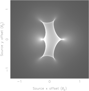
FIG. 6.: Magnification map as a function of source position for a typical binary lens. Axes show source offset from the lens centroid in units of Einstein angle $\theta_{E}$. Grey-scale shows magnification on a log scale, from 1 (black) to 10 (white). The lens consists of two point masses with $2:1$ mass ratio separated by $1\theta_{E}$ (defined using the total mass of the system); the larger mass is at (-1/3, 0) and the smaller at (+2/3, 0).

Clearly a binary lens can lead to a great diversity of lightcurves, since there are 3 additional free parameters; the mass ratio, the projected separation in units of the Einstein radius, and the orientation of the binary relative to the source path. However, caustic crossings are common features, which must occur in inward-outward pairs, so these events are quite easily recognised. Fitting of models to observed binary events is non-trivial due to the large parameter space and multiple minima [38].

To date, about 8 definite binary-lens events have been observed, OGLE-7 above, DUO-2 [2], MACHO LMC-9 below and about 5 by the MACHO alert system; there are several more probable cases where the data coverage is not quite sufficient to be certain.

A related effect is the case of lensing by a star with a planetary system; here the caustics are much smaller, so such an event appears like a single-lens event with some probability ($\sim 1-20\%$) of a short-lived deviation if one image passes near a planet. This is valuable since it is sensitive to smaller planet masses [17] than the recent planet discoveries via radial velocity measurements. Thus, to detect planets via microlensing, it is desirable to take existing microlensing alerts and observe them much more frequently ($\sim$ hourly); this is being undertaken by two teams, PLANET and GMAN.

VI LMC Results

The microlensing searches towards the LMC and SMC are the most important for the dark matter question, since these lines of sight pass mainly through the outer Galaxy where the density is dominated by dark matter; thus, unlike the bulge case, the lensing rate for an all-MACHO halo is much larger than that from known stars.

At present, we have analysed the first 2.3 years of data for our ‘high priority’ LMC fields; this sample contains some 8.5 million stars with 300–800 observations each [8]. A set of automated selection criteria applied to this sample yields 12 objects; 2 of these are redundant detections of two stars which appear in field overlaps and are independently analysed, and a further 2 are rejected due to ‘magnification bias’ in that they were brighter than normal in our template image and have subsequently faded below our detection limit (one of these was almost certainly a supernova in a background galaxy). This leaves 8 candidate microlensing events, which are shown in Fig. 7. (These are numbered 1,4–10 since two low-quality candidates 2 & 3 appeared in an earlier paper but no longer pass the improved selection criteria).

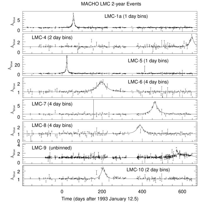
FIG. 7.: Lightcurves (observed flux vs time) for the eight candidate microlensing events from the 2-year Large Magellanic Cloud data. Data points ($\pm 1\sigma$ errors) show flux in linear units, relative to the fit baseline. For clarity, flux data have been averaged in time bins of width 1-4 days roughly scaled with the event durations (see labels). Only data in one colour is shown. The curves show the single-lens microlensing fit to each event. (From [8]).

Here event 1 is the event first announced in [3]; the star’s spectrum shows no abnormalities [23]. Event 4 was discovered by our Alert system, thus has more accurate follow-up observations (not shown here) which support the microlensing interpretation. Event 5 occurs in a faint star but has a very high peak magnification; the magnification appears slightly greater in the blue passband than in the red, probably due to blending. Event 9 is due to a binary lens; the fit shown in Fig. 7 is the single-lens fit used in event detection, thus is not appropriate. Events 6, 7 and 8 are good-quality candidates, while event 10 appears somewhat asymmetrical and may be a variable star; the inclusion or exclusion of this event has little effect on the results. The distribution of these candidates across the colour-magnitude diagram and in $A_{\rm max}$ is consistent with the microlensing predictions given in Section IIB. Some four of these candidates (1,4,5,9) are of high quality and are almost certainly due to microlensing; this suggests that most of the lower quality candidates are also microlensing, since if only the high-magnification candidates were actually microlensing while the others were variable stars, the implied distribution of $A_{\rm max}$ would be somewhat improbable.

Given observed microlensing events, it is natural to ask whether the individual lenses can be detected post-hoc, either directly or by their microlensing other nearby stars. Unfortunately, direct detection is unlikely since the lenses may be $1-6$ orders of magnitude fainter than the source star, and the relative angular velocity (“proper motion” in astronomical jargon) would be $\sim 0.005$ arcsec/yr; thus even after a decade they would be only marginally resolved by HST. Likewise, it will take centuries for a given lens to reach a neighbouring source star, and even then it is improbable that the alignment would be close enough to lens the second star.

To obtain quantitative conclusions, we clearly need to assess our event detection efficiency. The detection probability for individual events is a complicated function of $A_{\rm max}$, $\widehat{t}\,$, the observing strategy and the brightness of the source star, but all these distributions except $\widehat{t}\,$ are known, and thus can be averaged over by a Monte-Carlo simulation. There are two levels of detail here: firstly a ‘sampling efficiency’ which assumes all stars are single sources and adds events at the time-series level; and secondly a ‘blending efficiency’ which adds artificial stars into the raw image data. The latter is more realistic, but typically only differs by $\sim 15\%$ from the sampling efficiency, since there is an approximate cancellation between the increased number of stars in a blend and the reduction in observed magnification. The event detection efficiency ${\cal E}(\widehat{t}\,)$ is shown in Fig. 8, and shows a broad peak between $\widehat{t}\,\sim 30-300$ days.

Given a model for the halo density profile and velocity dispersion, it is straightforward to predict the event rate and distribution of timescales $\widehat{t}\,$ for arbitrary lens mass; combined with the efficiency function, this gives an expected number of events $N_{\rm exp}$. In practice it is convenient to show the expected number of events $\tilde{N}(M)$ for an all-MACHO halo in which all MACHOs have a unique mass $M$, which is shown in Fig. 9. Note that $\tilde{N}(M)$ peaks at $\tilde{N}>40$ for $M\sim 0.001-0.01\,{\rm M_{\odot}}$; the reason is that for $M\mathrel{\hbox{\hbox to0.0pt{\hbox{\lower 4.0pt\hbox{$\sim$}}\hss}\hbox{$>$}}}0.1\,{\rm M_{\odot}}$, most events are longer than 30 days where the efficiency curve is quite flat, while the event rate is falling $\propto M^{-1/2}$. For small masses $M\mathrel{\hbox{\hbox to0.0pt{\hbox{\lower 4.0pt\hbox{$\sim$}}\hss}\hbox{$<$}}}10^{-3}\,{\rm M_{\odot}}$, the theoretical event rate is large but most events are shorter than 3 days where the efficiency is very low. The product of these two factors gives the peak in $\tilde{N}(M)$.

FIG. 8.: Detection efficiency vs event duration ${\cal E}(\widehat{t}\,)$ for the LMC 2-year data. The dotted line shows the “photometric” efficiency assuming all stars are single, while the solid line incorporates the effects of blending. The efficiency is defined relative to the theoretical event rate with $u_{\rm min}<1$, and thus contains a factor of $0.66$ from the actual cut $A_{\rm max}>1.75$ or $u_{\rm min}<0.66$. (From [8]).

FIG. 9.: Upper panel: the expected number of microlensing events vs MACHO mass $\tilde{N}(M)$, including detection efficiency, for an all-MACHO dark halo with unique MACHO mass. The solid line shows total number of events, the dotted line shows events with duration $\widehat{t}\,<20$ days. Lower panel: resulting limits on the fraction of the halo contributed by MACHOs of given mass; regions above the curves are excluded at $95\%$ CL. The solid line is derived from 8 events total, the dashed line from no observed events with $\widehat{t}\,<20$ days. (From [8]).

There are several complementary ways to analyse a set of detected microlensing events: firstly, one may obtain robust upper limits for given $M$ by simply excluding models which predict too many detected events, shown in the lower panel of Figure 9. For substellar MACHOs we may obtain stronger limits since most events should have short duration ($\widehat{t}\,<20$ days), but we have no candidate event shorter than this. The dotted lines in Fig. 9 show the expected number of events with $\widehat{t}\,<20$ days, and the resulting limit: objects in the mass range $10^{-4}-0.01\,{\rm M_{\odot}}$ comprise $<20\%$ of a standard dark halo, and this applies whatever the shape of the mass function. We have extended this constraint to smaller masses using a separate search for very short duration events, called a ‘spike’ analysis; since many fields were observed twice per night, we can search for sets of four data points (two red-blue pairs) from a single night which show a significant brightening in all four points. There is insufficient data here to obtain a microlensing fit, so if events were found we could not claim a detection; but using suitable selection criteria, no such events are found, which allows us to extend the excluded region down to around $10^{-6}\,{\rm M_{\odot}}$, as shown in Fig. 10 [7]. Similar (nearly independent) limits have been obtained by EROS [46].

FIG. 10.: Upper limits on low-mass MACHOs based on the non-detection of very short duration ‘spike’ events, and no events with $\widehat{t}\,<20$ days in the standard search. The lines show the $95\%$ c.l. upper limit on the total mass of MACHOs within $50\,{\rm kpc}$ of the galactic center, as a function of the assumed MACHO mass, for 8 different models of the dark halo. (From [7]).

Secondly, one may obtain an unbiased estimate of the optical depth by

$$\tau_{\rm est}={\pi\over 4E}\sum_{i}{\widehat{t}\,_{i}\over{\cal E}(\widehat{t}\,_{i})}$$ (16)

where $\widehat{t}\,_{i}$ is the timescale of the $i$th event and $E$ is the ‘exposure’ in star-years. For the LMC 2-year sample this gives $\tau_{\rm LMC}\approx 2.9^{+1.4}_{-0.9}\,\times 10^{-7}$. This quantity has the virtue of being independent of assumptions about lens masses and velocity distributions; the drawback is that it is subject to non-Poisson statistics, and also does not account for contributions from timescales outside the window of sensitivity where ${\cal E}\rightarrow 0$. Thus, we caution that it is not valid to convert $\tau_{\rm est}$ into a constraint on the total abundance of MACHOs without specifying an associated mass interval; unfortunately this over-general statement sometimes appears in the literature.

The most dramatic result here is that the $\tau_{\rm est}$ above is not much smaller than the value in Eqn. 11, and both $\tau_{\rm est}$ and the number of 8 observed events substantially exceeds expectations from lensing by ‘known’ low-mass stars. Lensing by stars is estimated to contribute $\tau_{\rm stars}\approx 0.5\,\times 10^{-7}$ or around $1.1$ event to the above sample; hence there appears to be a very significant excess. Thus, one may treat the events as a detection of halo dark matter and use a maximum likelihood model to estimate the most probable MACHO mass $M$ and MACHO fraction of the halo $f$. Assuming a unique mass for all MACHOs, the result is shown in Fig. 11, and is $M=0.5^{+0.3}_{-0.2}\,{\rm M_{\odot}}$, $f=0.5^{+0.3}_{-0.2}$. A common source of confusion here is that that the 95% c.l. excluded region in Fig. 9 is not simply the complement of the $95\%$ allowed region in Fig. 11. The reason is that the unknown MACHO fraction of the halo is really a function $\psi(M)$ (with $f=\int\psi(M)dM$), not a point in 2-parameter space $f,M$. The likelihood analysis depends on the shape of $\psi(M)$ through the event timescales; this is unknown a priori and we must adopt some simple parametrisation, e.g. a $\delta$-function or a truncated power law. If we assume a different shape for the mass function, the ‘allowed region’ in the likelihood analysis may change, but the excluded region in Fig. 9 does not. Thus one needs both analyses to extract the full information from the data.

FIG. 11.: Likelihood contours for MACHO mass $M$ and the fraction of the halo comprised of MACHOs $f$, for a standard model halo with a $\delta-$function MACHO mass distribution. The lower panel assumes all 8 events are due to halo lenses, the upper panel assumes 6 such events. (From [8]).

VII Discussion

The interpretation of the LMC results is currently unclear. One conclusion is robust, that MACHOs in the planetary mass range $10^{-6}$ to $0.05\,{\rm M_{\odot}}$ do not contribute a substantial fraction of the Galactic dark halo. Regarding the detected events, although the Poisson uncertainties are substantial, this is not the dominant uncertainty: the critical question is, to what population of objects do most of the lenses belong ? As noted above, the 8 events in the 2-year data are substantially in excess of the predicted ‘background’ of $\approx 1.1$ event arising from known stellar populations, which suggests that MACHOs in a dark halo are a natural explanation.

However, there are some astrophysical difficulties with this interpretation, mainly arising from the estimated mass $\sim 0.5\,{\rm M_{\odot}}$ for the lenses. These cannot be hydrogen-burning stars in the halo since such objects are limited to $<3\%$ of the halo mass by deep star counts [31]. Modifying the halo model to slow down the lens velocities can reduce the implied lens mass somewhat, but probably not below the substellar limit $0.08\,{\rm M_{\odot}}$. Old white dwarfs have about the right mass and can evade the direct-detection constraints, but it is difficult to form them with high efficiency, and there may be problems with overproduction of metals and overproduction of light at high redshifts from the luminous stars which were the progenitors of the white dwarfs [21]. Primordial black holes are a viable possibility, though one has to appeal to a coincidence to have them in a stellar mass range.

Due to these difficulties of getting MACHOs in the inferred mass range without violating other constraints, there have been a number of suggestions for explaining the LMC events without recourse to a dark population: most of these suggestions construct some non-standard distribution of ‘ordinary’ stars along the LMC line of sight, to increase the stellar lensing rate. Fairly general arguments from faint star counts can limit the contribution from our Milky Way disk [31]. The contribution from LMC ‘self-lensing’, i.e. stars in the front of the LMC lensing those in the back, is less well constrained: [47] estimated an optical depth $\sim 0.5\,\times 10^{-7}$ from this, but this has been disputed by [30] who obtains an upper limit of $0.25\,\times 10^{-7}$ using dynamical constraints. This can be tested given more data via the distribution of events on the sky, since lenses in the LMC itself should be concentrated towards the center of the LMC. Other suggested lens populations include an unknown dwarf galaxy roughly half-way to the LMC [59], a tidal tail of stars stripped from the LMC [60], or a strongly flared and warped disk of our Galaxy [24]. All of these proposals appear somewhat contrived but can be tested observationally in the near future.

However, the most decisive test for the lens population is to break the degeneracy in $M,l,v_{\perp}$ and thus estimate the distance to at least a subsample of the lenses. This can be done for ‘non-standard’ lensing events using the methods outlined in Sec. V, but the percentage of events showing such deviations is expected to be small, especially for halo lenses. The ideal method for measuring lens locations is to discover lensing events in real time, as already happens, and then make extra observations from a small satellite at $\mathrel{\hbox{\hbox to0.0pt{\hbox{\lower 4.0pt\hbox{$\sim$}}\hss}\hbox{$>$}}}0.3$ AU from the Earth [29]. Since this distance is comparable to the Einstein radius of the lens, the event lightcurve will appear substantially different from the satellite and the Earth, e.g. the times of peak brightness are expected to differ by $\sim 1$ week. As with the parallax effect of Section V, this yields a measurement of the ‘projected’ velocity of the lens across the Solar system $v_{\perp}/(1-x)$. This can unambiguously determine whether the lens belongs to our disk, the halo or the LMC. Another possibility is that planned space astrometric missions such as SIM [42] and GAIA should be able to measure the deflection of the light centroid $\sim 10^{-4}$ arcsec [56] during a microlensing event, which gives a measurement of the angular Einstein radius $\theta_{E}$ and thus the lens angular velocity $v_{\perp}/l$. Measuring both parallax and $\theta_{E}$ for the same event gives a complete solution for $M$, $l$ and $v_{\perp}$.

The prospects for microlensing appear bright: the MACHO project will continue to observe until at least 1999, and the EROS-2 and OGLE-2 telescopes have recently come on line, which should significantly increase the event rate, reducing the statistical uncertainties and enabling useful tests for the distribution of lenses across the LMC. Microlensing searches in new directions are also starting to produce results, including the first event towards the SMC [10, 43] and candidate events towards M31 [52]. The suggestions for stellar lensing populations can be tested observationally, though if these populations are not found we may need to wait a few years for one of the space-based missions to finally decide whether the lenses are in the dark halo.

- [1]
- Alard et al. [1996] Alard, C., S. Mao & J. Guibert, 1996, Astron. Astrophys. 300, L17.
- Alcock et al. [1993] Alcock, C. et al. (MACHO Coll.), 1993, Nature365, 621.
- Alcock et al. [1995a] Alcock, C. et al. (MACHO Coll.), 1995a, Phys. Rev. Lett.74, 2867.
- Alcock et al. [1995b] Alcock, C. et al. (MACHO Coll.), 1995b, ApJ454, L125.
- Alcock et al. [1996a] Alcock, C. et al. (MACHO Coll.), 1996a, ApJ463, L67.
- Alcock et al. [1996b] Alcock, C. et al. (MACHO Coll.), 1996b, ApJ471, 774.
- Alcock et al. [1997a] Alcock, C. et al. (MACHO Coll.), 1997a, ApJ486, 697.
- Alcock et al. [1997b] Alcock, C. et al. (MACHO Coll.), 1997b, ApJ479, 119.
- Alcock et al. [1997c] Alcock, C. et al. (MACHO Coll.), 1997c, ApJ491, L11.
- Alcock et al. [1998a] Alcock, C. et al. (MACHO Coll.), 1998a, ApJ491, 436.
- Ashman [1992] Ashman, K.M., 1992, Pubs. Astron. Soc. Pacific 104, 1109.
- Aubourg et al. [1993] Aubourg, E. et al. (EROS Coll.), 1993, Nature365, 623.
- Ansari et al. [1996] Ansari, R. et al. (EROS Coll.), 1996, Astron. Astrophys. 314, 94.
- Benetti, Pasquini & West [1995] Benetti, S., L. Pasquini & R.M. West, 1995, Astron. Astrophys. 294, L37.
- Bennett et al. [1995] Bennett, D.P. et al. (MACHO Coll.), 1995, in “Dark Matter”, AIP Conf. Proc. 316, American Inst. of Physics, New York.
- Bennett & Rhie [1996] Bennett, D.P. & S.-H. Rhie, 1996, ApJ472, 660.
- Blandford & Narayan [1992] Blandford, R.D. & R. Narayan, 1992, Annual Rev. Astron. Astrophys. 30, 311.
- Carlberg et al. [1998] Carlberg, R.G. et al., 1998, in “Large-Scale Structure: Tracks and Traces”, 12th Potsdam Cosmology Workshop, ed V. Mueller (World Scientific).
- Carr [1994] Carr, B., 1994, Annual Rev. Astron. Astrophys. 32, 531.
- Charlot & Silk [1995] Charlot, S. & J. Silk, 1995, ApJ445, 124.
- Cook et al. [1997] Cook, K. et al., 1997, in “Variable Stars and the Astrophysical Returns of Microlensing Surveys”, 12th IAP Colloquium, eds. R. Ferlet & J-P. Maillard (Editions Frontieres, Gif-sur-Yvette).
- Della Valle [1994] Della Valle, M., 1994, Astron. Astrophys. 287, L31.
- Evans et al. [1998] Evans, N.W., G. Gyuk, M.S. Turner & J.J. Binney, 1998, ApJ, 501, L45.
- Flynn, Gould & Bahcall [1996] Flynn, C., A. Gould & J.N. Bahcall, 1996, ApJ466, L55.
- Griest [1991] Griest, K., 1991, ApJ366, 412.
- Gould [1992] Gould, A., 1992, ApJ, 392, 442.
- Gould [1994a] Gould, A., 1994a, ApJ421, L71.
- Gould [1994b] Gould, A., 1994b, ApJ421, L75.
- Gould [1995b] Gould, A., 1995b, ApJ441, 77.
- Gould, Bahcall & Flynn [1997] Gould, A., J.N. Bahcall & C. Flynn, 1997, ApJ482, 913.
- Han & Gould [1996] Han, C. & A. Gould, 1996, ApJ467, 540.
- Han & Gould [1997] Han, C. & A. Gould, 1997, ApJ480, 196.
- Hart et al. [1996] Hart, J. et al., 1996, Pubs. Astron. Soc. Pacific 108, 220.
- Hewitt et al. [1988] Hewitt, J.N., E.L. Turner, D.P. Schneider, B.F. Burke, G.I. Langston, 1988, Nature333, 537.
- Jungman et al. [1996] Jungman, G.U., M. Kamionkowski & K. Griest, 1996, Phys. Rep. 267, 195.
- Kochanek & Hewitt [1996] Kochanek, C.S. & J.N. Hewitt, eds, 1996. “Astrophysical Applications of Gravitational Lensing”, IAU Symp. 173. (Kluwer, Dordrecht).
- Mao & Di Stefano [1995] Mao, S. & R. Di Stefano, 1995, ApJ440, 22.
- Mao & Paczynski [1991] Mao, S. & B. Paczynski, B., 1991, ApJ374, L37.
- Paczynski [1986] Paczynski, B., 1986, ApJ304, 1.
- Paczynski [1996] Paczynski, B., 1996, Annual Rev. Astron. Astrophys. 34, 419.
- Paczynski [1998] Paczynski, B., 1998, ApJ, 494, L23.
- Palanque-Delabrouille et al. [1998] Palanque-Delabrouille, N. et al. (EROS coll.), 1998, Astron. Astrophys. , in press.
- Peebles [1993] Peebles, P.J.E., 1993. “Principles of Physical Cosmology”. (Princeton Univ. Press).
- Refsdal [1964] Refsdal, S., 1964, Monthly Notices Royal Astron. Soc. 128, 295.
- Renault et al. [1997] Renault, C. et al. (EROS Coll.), 1997, Astron. Astrophys. 324, L69.
- Sahu [1994] Sahu, K.C., 1994, Nature370, 275.
- Schechter, Mateo & Saha [1993] Schechter, P.L., M. Mateo & A. Saha, 1993, Pubs. Astron. Soc. Pacific 105, 1342.
- Schneider & Weiss [1986] Schneider, P. & A. Weiss, 1986, Astron. Astrophys. 164, 237.
- Strauss & Willick [1995] Strauss, M.A. & J.A. Willick, 1995, Phys. Rep. 261, 271.
- Stubbs et al. [1993] Stubbs, C.W. et al., 1993, Proc. SPIE 1900, 192.
- Tomaney & Crotts [1996] Tomaney, A.B. & A.P.S. Crotts, 1996, Astron. J. 112, 2872.
- Udalski et al. [1993] Udalski, A., M. Szymanski, J. Kaluzny, M. Kubiak, W. Krzeminski, M. Mateo, G.W. Preston & B. Paczynski, 1993, Acta Astronomica 43, 289.
- Udalski et al. [1994a] Udalski, A., M. Szymanski, J.Kaluzny, M. Kubiak, W. Krzeminski, M. Mateo, G.W. Preston & B. Paczynski, 1994a, Acta Astronomica 44, 165.
- Udalski et al. [1994b] Udalski, A., M. Szymanski, S. Mao, R. di Stefano, J. Kaluzny, M. Kubiak, M. Mateo & W. Krzeminski, 1994b, ApJ436, L103.
- Walker [1995] Walker, M.A., 1995, ApJ453, 37.
- Walsh, Carswell & Weymann [1979] Walsh, D., R.F. Carswell & R.J. Weymann, 1979, Nature279, 381.
- Witt & Mao [1994] Witt, H.J. & S. Mao, 1994, ApJ430, 505.
- Zhao [1998a] Zhao, H.-S., 1998a, Monthly Notices Royal Astron. Soc. , 294, 139.
- Zhao [1998b] Zhao, H.-S., 1998b, preprint (astro-ph/9703097)