Hyperextended Cosmological Perturbation Theory:
Predicting Non-linear Clustering Amplitudes

Abstract

We consider the long-standing problem of predicting the hierarchical clustering amplitudes $S_{p}$ in the strongly non-linear regime of gravitational evolution. N-body results for the non-linear evolution of the bispectrum (the Fourier transform of the three-point density correlation function) suggest a physically motivated ansatz that yields the strongly non-linear behavior of the skewness, $S_{3}$, starting from leading-order perturbation theory. When generalized to higher-order ($p>3$) polyspectra or correlation functions, this ansatz leads to a good description of non-linear amplitudes in the strongly non-linear regime for both scale-free and cold dark matter models. Furthermore, these results allow us to provide a general fitting formula for the non-linear evolution of the bispectrum that interpolates between the weakly and strongly non-linear regimes, analogous to previous expressions for the power spectrum.

CITA-98-17, FERMILAB-Pub-98/255-A

1 Introduction

Analytic understanding of gravitational clustering in the strongly non-linear regime remains an elusive goal in the study of large-scale structure. While the growth of structure in the weakly non-linear regime, where the density field contrast $\delta\mathrel{\mathchoice{\lower 3.6pt\vbox{\halign{$\mathsurround=0pt\displaystyle\hfill#\hfil$\cr<\crcr\sim\crcr}}}{\lower 3.6pt\vbox{\halign{$\mathsurround=0pt\textstyle\hfill#\hfil$\cr<\crcr\sim\crcr}}}{\lower 3.6pt\vbox{\halign{$\mathsurround=0pt\scriptstyle\hfill#\hfil$\cr<\crcr\sim\crcr}}}{\lower 3.6pt\vbox{\halign{$\mathsurround=0pt\scriptscriptstyle\hfill#\hfil$\cr<\crcr\sim\crcr}}}}1$, is well described by cosmological perturbation theory (Juszkiewicz, Bouchet & Colombi (1993); Bernardeau (1994), 1994b; Baugh, Gaztañaga & Efstathiou (1995); Gaztañaga & Baugh (1995); Juszkiewicz et al. (1995); Łokas et al. (1995)), corresponding progress has not been made in understanding clustering when $\delta\gg 1$. This lack of progress traces in part to the relative complexity and intractability of the coupled BBGKY hierarchy of equations for the phase space distribution functions (Peebles 1980); moreover, with the development of high-resolution N-body simulations, the non-linear gravitational evolution can now be tracked directly. However, simulations provide only limited physical insight into the complex non-linear phenomena involved in gravitational clustering. To the extent possible, one would like a qualitative and ideally quantitative understanding of non-linear clustering from first principles. Analytic models can also provide a useful check on simulation results, which have their own intrinsic limitations and uncertainties.

Recently, cosmological perturbation theory has been extended further into the non-linear regime through the inclusion of next-to-leading order corrections: one-loop perturbative calculations of the power spectrum (Makino et al. (1992); Łokas et al. (1996); Scoccimarro & Frieman (1996)), bispectrum (Scoccimarro (1997); Scoccimarro et al. (1998), hereafter SCFFHM) and skewness (Scoccimarro & Frieman 1996a ; Scoccimarro (1997); Fosalba & Gaztañaga (1998)) have been found to be in excellent agreement with N-body results even in the regime where the variance $\sigma^{2}\equiv\langle\delta^{2}(R)\rangle\sim 1$ for the bispectrum and as large as $\sigma^{2}\sim 10$ for the power spectrum (where $\delta(R)$ is the density field contrast smoothed through a window of radius $R$). However, it is clear that perturbation theory cannot be pushed successfully beyond this point to calculate clustering amplitudes in the strongly non-linear regime. The perturbation series is at best asymptotic, and it is expected to break down on small scales, where $\sigma^{2}\gg 1$. More importantly, the single-stream fluid approximation, upon which the perturbative solutions are based, must fail on small scales where shell-crossing occurs, and be replaced with the BBGKY equations.

Nevertheless, non-linear gravitational clustering does appear to display striking scaling properties, and some success has been achieved in combining perturbation theory with concepts such as stable clustering to make predictions about strongly non-linear behavior. The stable clustering hypothesis states that on very small scales, where clustering has reached virial equilibrium, the mean relative velocity between pairs should exactly cancel the Hubble expansion. When coupled with the equations of motion, this leads to general predictions for the growth of the hierarchy of $p$-point density correlation functions (Peebles 1980). For scale-free initial conditions, i.e., power spectrum $P_{i}(k)\sim k^{n}$, in an Einstein-de Sitter universe (with $\Omega_{m}=1$), it follows from self-similarity that the slope of the non-linear two-point function, $\xi(r)\sim r^{-\gamma}$, is related to the spectral index $n$ of the initial perturbations by $\gamma=3(n+3)/(n+5)$ (Davis & Peebles 1977). For a range of initial spectra $n$, the results of N-body simulations are consistent with this self-similar solution in the strongly non-linear regime, $\xi\mathrel{\mathchoice{\lower 3.6pt\vbox{\halign{$\mathsurround=0pt\displaystyle\hfill#\hfil$\cr>\crcr\sim\crcr}}}{\lower 3.6pt\vbox{\halign{$\mathsurround=0pt\textstyle\hfill#\hfil$\cr>\crcr\sim\crcr}}}{\lower 3.6pt\vbox{\halign{$\mathsurround=0pt\scriptstyle\hfill#\hfil$\cr>\crcr\sim\crcr}}}{\lower 3.6pt\vbox{\halign{$\mathsurround=0pt\scriptscriptstyle\hfill#\hfil$\cr>\crcr\sim\crcr}}}}10-100$ (Efstathiou et al. 1988; Colombi, Bouchet, & Hernquist (1996), hereafter CBH; Jain 1997; Couchman & Peebles (1998)). In current models of structure formation, such as cold dark matter (CDM) and its variants, the initial power spectrum is not precisely scale-free. Nevertheless, the spectral index $n=d\ln P/d\ln k$ generally varies slowly enough with scale that one expects scaling arguments to provide useful insight into non-linear clustering. In this paper, we use such considerations to study the non-linear evolution of higher-order correlations.

A classic problem in this context is the prediction of the strongly non-linear hierarchical amplitudes $S_{p}(R)=\langle\delta^{p}(R)\rangle/\langle\delta^{2}(R)\rangle^{p-1}$. For scale-free initial conditions in an Einstein-de Sitter universe, the stable clustering hypothesis extended to higher-order correlations (Peebles 1980, Jain 1997) implies that the $S_{p}$ should be constant, independent of $R$, in the strongly non-linear regime, $\sigma^{2}\gg 1$, but it does not say what the amplitudes are.

This result motivated several papers which attempted to calculate the hierarchical amplitudes from the equations of motion. Observations of galaxy clustering at small scales and the self-similarity solution of the BBGKY equations motivate the so-called hierarchical model for the connected $p$-point correlation function (Fry 1984b),

$$\kappa_{p}({\hbox{\BF x}}_{1},...,{\hbox{\BF x}}_{p})\equiv\langle\delta({\hbox{\BF x}}_{1}),...,\delta({\hbox{\BF x}}_{p})\rangle_{c}=\sum_{a=1}^{t_{p}}Q_{p,a}\sum_{\rm labelings}\ \prod_{\rm edges}^{p-1}\xi_{AB}\equiv Q_{p}\sum_{a=1}^{t_{p}}\ \sum_{\rm labelings}\ \prod_{\rm edges}^{p-1}\xi_{AB}.$$ (1)

The product is over $p-1$ edges that link $p$ galaxies (vertices) $A,B,...$, with a two-point correlation function $\xi_{XY}$ assigned to each edge. These configurations can be associated with ‘tree’ graphs, called $p$-trees. Topologically distinct $p$-trees, denoted by $a$, in general have different amplitudes, denoted by $Q_{p,a}$, but those configurations which differ only by permutations of the labels 1,…,$p$ (and therefore correspond to the same topology) have the same amplitude. There are $t_{p}$ distinct $p$-trees ($t_{3}=1$, $t_{4}$=2, etc., see Fry (1984b) and Boschán, Szapudi & Szalay 1994) and a total of $p^{p-2}$ labeled trees. The hierarchical model represents the connected $p$-point functions as sums of products of $(p-1)$ two-point functions, introducing at each level only as many extra parameters $Q_{p,a}$ as there are distinct topologies. In what we shall call the degenerate hierarchical model, the amplitudes $Q_{p,a}$ are furthermore independent of scale and configuration. In this case, $Q_{p,a}=Q_{p}$, and the hierarchical amplitudes $S_{p}\simeq p^{p-2}\ Q_{p}$. In the general case, the amplitudes $Q_{p}$ depend on overall scale and configuration. For example, for Gaussian initial conditions, in the weakly non-linear regime, $\sigma^{2}\ll 1$, perturbation theory predicts a clustering pattern that is hierarchical but not degenerate.

Using the BBGKY hierarchy and assuming a hierarchical form similar to Eq. (1) for the phase-space $p$-point distribution function, in the stable clustering limit Fry (1982, 1984) obtained ($p\geq 3$)

$$Q_{p}=Q_{p,a}=\frac{1}{2}\ \Big{(}\frac{p}{p-1}\Big{)}\ \Big{(}\frac{4Q_{3}}{p}\Big{)}^{p-2};$$ (2)

in this case, different tree diagrams all have the same amplitude, i.e., the clustering pattern is degenerate. On the other hand, Hamilton (1988), correcting an unjustified symmetry assumption in Fry (1982, 1984), instead found

$$Q_{p,{\rm snake}}=Q_{3}^{p-2},\ \ \ \ \ Q_{p,{\rm star}}=0$$ (3)

where “star” graphs correspond to those tree graphs in which one vertex is connected to the other $(p-1)$ vertices, the rest being “snake” graphs. Summed over the snake graphs, (3) yields

$$Q_{p}=\frac{p!}{2}\ \Big{(}\frac{Q_{3}}{p}\Big{)}^{p-2}.$$ (4)

Unfortunately, as emphasized by Hamilton (1988), these results are not physically meaningful solutions to the BBGKY hierarchy, but rather a direct consequence of the assumed factorization in phase-space. As a result, this approach leads to unphysical predictions such as that cluster-cluster correlations are equal to galaxy-galaxy correlations to all orders. It remains to be seen whether physically relevant solutions to the BBGKY hierarchy which satisfy Eq. (1) really do exist. Despite these shortcomings, the results in Eq. (2) and Eq. (3) are often quoted in the literature as physically relevant solutions to the BBGKY hierarchy!

The complexity of the BBGKY equations has prompted a phenomenological approach to the description of correlation functions based on the hierarchical model. An example is the factorizable hierarchical model (Bernardeau & Schaeffer 1992), which is completely specified by the star amplitudes. In this case the snake amplitudes at any given order are determined by the lower order star amplitudes, $Q_{p,a}=\Pi_{i}\nu_{i}^{d_{i}(a)}$, where $\nu_{i}$ are the vertex weights for $i$ lines and $d_{i}(a)$ is the number of such vertices in diagrams with topology denoted by $a$. This is analogous to the pattern that emerges from PT at large scales, although the parameters $Q_{p,a}$ are in this case taken to be constant, independent of scale and configuration, as in the spherical model.

A more general framework than the hierarchical model is given by the scale-invariant model (Balian & Schaeffer 1989), in which the connected $p$-point function obeys the scaling law

$$\kappa_{p}(\lambda{\hbox{\BF x}}_{1},...,\lambda{\hbox{\BF x}}_{p})=\lambda^{-(p-1)\gamma}\ \kappa_{p}({\hbox{\BF x}}_{1},...,{\hbox{\BF x}}_{p}),$$ (5)

where $\gamma$ is the index of the two-point function, $\xi(r,t)\sim(r/t^{\alpha})^{-\gamma}$, with $\alpha=4/[3(n+3)]$. Eq. (5) is the self-similar solution to the BBGKY hierarchy, which holds in the case of stable clustering for scale-free initial conditions in an Einstein-de Sitter universe (Peebles 1980). The hierarchical model of Eq. (1) satisfies Eq. (5), but the latter is more general and can be satisfied by other functional forms than Eq. (1).

The best observational constraints on higher-order galaxy correlation functions in the non-linear regime currently come from angular surveys, although this situation will soon change dramatically with the advent of large redshift surveys such as the Two Degree Field (2dF) and Sloan Digital Sky Survey (SDSS). Measurement of the angular three-point function (Groth & Peebles 1977) and four-point function (Fry & Peebles 1978) in the Lick survey provided the first observational evidence for the scale-invariant model of Eq. (5). Moreover, these observations are consistent with the hierarchical model, with $Q_{3}\approx 1.3$ and $Q_{4}\approx 3$. More recently, Gaztañaga (1994) measured the $S_{p}$ parameters ($3\leq p\leq 9$) in the APM galaxy survey and found good agreement with the scale-invariant model at small scales. Szapudi & Szalay (1998) investigated the third- and fourth-order cumulant correlators in the APM and found $Q_{3}\approx 1$ and $Q_{4}\approx 3$, in good agreement with the Lick survey results. On the other hand, when decomposing the average four-point amplitude $Q_{4}$ into the two different topologies, Szapudi & Szalay (1998) (see also Szapudi et al. 1995) found $R_{a}=Q_{4,{\rm snake}}=3.7$ (for the snake topology) and $R_{b}=Q_{4,{\rm star}}=0.8$ (star topology), whereas Fry & Peebles (1978) obtained $R_{a}=2.5\pm 0.6$ and $R_{b}=4.3\pm 1.2$ for the Lick survey. One must keep in mind, however, that these two measurements differ in the type of four-point configurations they considered (that is, they did not test the hierarchical ansatz in its full generality), so it remains possible that a finer measurement of the four-point function as a function of configuration could reconcile these discrepancies. Furthermore, in the EDSGC survey (which is based on a subset of the same photographic plates as used in the APM), Szapudi, Meiksin & Nichol (1996) found that $Q_{3}=2.0$, $Q_{4}=7.3$, substantially higher than in the APM (see Szapudi & Gaztañaga 1998 for a detailed comparison of higher order correlations in these two surveys). The upcoming 2dF and SDSS redshift surveys will be able to probe higher-order correlations with unprecedented accuracy and should help resolve these issues (Colombi, Szapudi, & Szalay (1998)). We note, however, that testing the hierarchical model in these cases will require redshift distortions to be taken into account; in particular, the large internal velocity dispersion of galaxy clusters leads to a strong configuration-dependence of the $Q_{p}$ amplitudes at small scales (Scoccimarro, Couchman & Frieman (1998)). In fact, this expected violation of the (degenerate) hierarchical ansatz is seen in the three-point function measured in the Las Campanas Redshift Survey (Jing & Börner 1998).

In this paper, we combine cosmological perturbation theory with the observed scaling behavior of the three-point function in N-body simulations to extract predictions for the non-linear clustering amplitudes $S_{p}$ for scale-free and CDM initial power spectra. The end result is a simple analytic expression for $S_{p}$ which appears to be valid at $\sigma^{2}\mathrel{\mathchoice{\lower 3.6pt\vbox{\halign{$\mathsurround=0pt\displaystyle\hfill#\hfil$\cr>\crcr\sim\crcr}}}{\lower 3.6pt\vbox{\halign{$\mathsurround=0pt\textstyle\hfill#\hfil$\cr>\crcr\sim\crcr}}}{\lower 3.6pt\vbox{\halign{$\mathsurround=0pt\scriptstyle\hfill#\hfil$\cr>\crcr\sim\crcr}}}{\lower 3.6pt\vbox{\halign{$\mathsurround=0pt\scriptscriptstyle\hfill#\hfil$\cr>\crcr\sim\crcr}}}}10$ when compared with N-body results. Along the way, we also provide fitting formulae for the non-linear evolution of the bispectrum, the Fourier transform of the three-point function, in the spirit of the two-point results of Hamilton et al. (1991), Jain, Mo & White (1995), and Peacock & Dodds (1994, 1996).

In recent work, Colombi et al. (1997) take a very different approach to ‘extending’ perturbative expressions for the $S_{p}$ parameters into the non-linear regime. In leading order perturbation theory (hereafter PT), valid for $\sigma^{2}\ll 1$, the $S_{p}$ are functions of the linear spectral index, $n=-3-d\ln\sigma^{2}_{\ell}(R)/d\ln R$, where $\sigma^{2}_{\ell}(R)$ denotes the linear variance at smoothing scale $R$ (Bernardeau 1994). Colombi, et al. find that the non-linear evolution of the $S_{p}$ can be fit with the same PT expressions provided they let the spectral index $n$ appearing therein become a free parameter as a function of the non-linear variance, $n\rightarrow n_{\rm eff}(\sigma^{2})$. (Note that $n_{\rm eff}$ is not the slope of the non-linear power spectrum.) The function $n_{\rm eff}(\sigma^{2})$, which depends on the initial spectrum, is extracted from, e.g., the measurement of $S_{3}(\sigma^{2})$ in an N-body simulation, assuming that the perturbative expression for the skewness remains valid throughout the non-linear regime, i.e., by fitting the N-body results to $S_{3}(\sigma^{2})=(34/7)-(n_{\rm eff}+3)$. Remarkably, they find that the extracted $n_{\rm eff}(\sigma^{2})$, when substituted into the PT expressions for the $S_{p}$ for $p>3$, provide a good fit to the non-linear (N-body) evolution of the higher-order moments as well. Similar behavior was noted for the EDSGC moments by Szapudi, Meiksin, and Nichol (1996). This extended perturbation theory (EPT) in principle provides a complete phenomenological description of one-point density field statistics, from linear to non-linear scales. (We describe it as a phenomenological model, because it is not a systematic development of perturbation theory for the non-linear regime; rather it is based upon the observation that the pattern of the $S_{p}$ in the non-linear regime is related by a single parameter to the pattern in the weakly non-linear (perturbative) regime.) Note that EPT does not give a predictive prescription for the non-linear $S_{p}$ for arbitrary initial conditions: if the initial conditions are changed, a new N-body simulation must be run in order to fit the function $n(\sigma^{2})$. In addition, it does not explictly describe the evolution of the multi-point functions.

The model discussed below, which we have dubbed “hyperextended perturbation theory” (HEPT), also contains phenomenological elements: it does not provide a rigorous, first-principles calculation of the strongly non-linear clustering amplitudes. However, it is based upon a simple physical picture of the non-linear evolution of the $N-$point functions that appears to hold quite generally. Thus, unlike extended perturbation theory, hyperextended perturbation theory yields an analytic prediction for the non-linear $S_{p}$ for arbitrary initial conditions.

This paper is organized as follows. Section 2 reviews the non-linear evolution of the bispectrum in PT and in N-body simulations and physically motivates the main ideas behind HEPT. In Section 3 we describe HEPT and present analytic results for the $S_{p}$ parameters in the non-linear regime, comparing them to measurements in numerical simulations. A fitting formula for the non-linear evolution of the bispectrum from the weakly to the strongly non-linear regime is given in Section 4. Finally, Section 5 presents our conclusions.

2 Extracting the Essence of HEPT: Non-Linear Evolution of the Bispectrum

We are interested in predicting the non-linear behavior of the higher-order correlations. For this purpose, we review here the non-linear evolution of the bispectrum, the Fourier transform of the three-point spatial correlation function, which is the lowest-order correlation function sensitive to phase information.

It is useful to first recall the nomenclature of higher order correlations in Fourier space. Defining the Fourier transform of the density contrast field by

$$\delta({\hbox{\BF k}})=\int\frac{d^{3}x}{(2\pi)^{3}}\ e^{-i{\hbox{\BF k}}\cdot{\hbox{\BF x}}}\ \delta({\hbox{\BF x}})~{},$$ (6)

the p^th order polyspectrum, $B_{p}$, is defined by the expectation value

$$\langle\delta({\hbox{\BF k}}_{1})\dots\delta({\hbox{\BF k}}_{p})\rangle=[\delta_{\rm D}]_{p}\ B_{p}({\hbox{\BF k}}_{1},\ldots,{\hbox{\BF k}}_{p}).$$ (7)

where $[\delta_{\rm D}]_{p}\equiv\delta_{D}({\hbox{\BF k}}_{1}+\dots+{\hbox{\BF k}}_{p})$. For $p=2$, this defines the power spectrum, and for $p=3$ the bispectrum. It is also convenient to define the $Q_{p}$ hierarchical amplitudes in Fourier space [see Eq. (1)] by ($p>2$)

$$Q_{p}\equiv\frac{B_{p}({\hbox{\BF k}}_{1},\ldots,{\hbox{\BF k}}_{p})}{\sum_{a=1}^{t_{p}}\ \sum_{\rm labelings}\prod_{\rm edges}^{p-1}P(k_{\rm AB}),}$$ (8)

where $P(k)$ is the power spectrum, and the sum in the denominator is over all the tree diagrams, as in Eq. (1). For example, $Q_{3}=B_{3}/(P_{1}P_{2}+P_{2}P_{3}+P_{3}P_{1})$, $Q_{4}=B_{4}/[P_{1}P_{2}P_{3}+({\rm 3~{}permutations})+P_{1}P_{12}P_{4}+({\rm 11~{}permutations})]$, and so on. Here $P_{i}\equiv P({\hbox{\BF k}}_{i})$ and $P_{ij}\equiv P({\hbox{\BF k}}_{i}+{\hbox{\BF k}}_{j})$. The hierarchical $S_{p}(R)$ parameters at smoothing scale $R$ are the one-point counterpart of the $Q_{p}$ amplitudes smoothed over a window of radius $R$:

$$S_{p}(R)\equiv\frac{\langle\delta^{p}(R)\rangle_{c}}{\langle\delta^{2}(R)\rangle^{p-1}}=\frac{\int B_{p}({\hbox{\BF k}}_{1},\ldots,{\hbox{\BF k}}_{p})\ W_{1}\ldots W_{p}\ [\delta_{\rm D}]_{p}\ d^{3}k_{1}\ldots d^{3}k_{p}}{[\int P(k)W(kR)^{2}d^{3}k]^{p-1}},$$ (9)

where $W_{i}\equiv W(k_{i}R)$, with $W(kR)$ the top-hat window function in Fourier space.

The non-linear evolution of $Q_{3}$ displays the main features expected to hold for higher-order polyspectra as well. As its behavior has been rather thoroughly studied in both PT and N-body simulations, we shall use the three-point function as a model to extrapolate to higher-order polyspectra. The $p>3$-order correlation functions become increasingly difficult to measure in numerical simulations for increasing $p$, so less is known about their non-linear evolution (however, see the studies of the four-point function by, e.g., Bromley (1994), Suto & Matsubara (1994), Munshi & Melott (1998)). On the other hand, there is partial information from studies of the evolution of one-point statistics such as the $S_{p}$ up to $p=10$ (Baugh, Gaztañaga & Efstathiou (1995); CBH).

There are basically three qualitatively distinct regimes for the non-linear evolution of $Q_{3}$:

a) Tree-Level. At large scales, leading-order (tree-level) PT provides an excellent description of gravitational clustering. In this regime, the $Q_{p}$ amplitudes in Eq. (8) are independent of the overall amplitude of the power spectrum. For scale-free initial conditions, $P_{k}(k)\sim k^{n}$, the PT $Q_{p}$ are scale-invariant but configuration-dependent, that is, they depend on the ratios $k_{i}/k_{j}$ and the angles ${\hbox{\BF k}}_{i}\cdot{\hbox{\BF k}}_{j}/(k_{i}k_{j})$ (Fry 1984b). The resulting $S_{p}$ parameters depend on scale only through the spectral index at the smoothing scale and its derivatives (Bernardeau (1994)), therefore they are constants for scale-free initial conditions.

b) One-Loop. By carrying the perturbative expansion for the $p-$point functions to next-to-leading order in the density contrast field, one includes the one-loop corrections to the tree-level results. One-Loop PT describes the dependence of $Q_{p}$ and $S_{p}$ on the amplitude of the power spectrum that appears at intermediate scales. Depending on the initial spectral index, one-loop corrections tend to enhance ($n_{\rm eff}~{}>~{}-1.4$) or reduce ($n_{\rm eff}~{}<~{}-1.4$) the tree-level configuration dependence of $Q_{3}$ (Scoccimarro 1997). For equilateral triangle configurations, one-loop PT describes the rise that connects the tree-level perturbative amplitude, $Q_{3}=4/7$, to the non-linear saturation value at small scales (SCFFHM). Similarly, one-loop corrections to the skewness $S_{3}$ describe the transition from its tree-level value to the non-linear regime (Scoccimarro 1997). Extension of this result within the spherical collapse approximation shows that one-loop corrections describe this transition region for $S_{p}$ with $p>3$ as well (Fosalba & Gaztañaga (1998)).

c) Saturation. At small scales, in the strongly non-linear regime, numerical simulations show that the $S_{p}(R)$ parameters reach a plateau, nearly independent of scale $R$; we refer to this behavior as “saturation”. The hierarchical amplitude $Q_{3}$ in this regime becomes constant to a good approximation, nearly independent of configuration (SCFFHM). Note, however, that it is still not settled whether the $S_{p}$ show small deviations from scale-invariant behavior in the strongly non-linear regime (CBH; Munshi et al. (1997)). From a theoretical point of view, as we discussed above, the only prediction in the strongly non-linear regime is from stable clustering, which implies that the $S_{p}$ should be constant for scale-free initial conditions in an Einstein-de Sitter model. As for the $Q_{p}$ parameters, however, stable clustering only constrains them to be scale-invariant (not necessarily hierarchical); in particular, for the bispectrum this implies

$$B(k_{1},k_{2},k_{3})=P(k_{1})P(k_{2})\ {\cal S}(r_{12},\theta_{12})+P(k_{2})P(k_{3})\ {\cal S}(r_{23},\theta_{23})+P(k_{3})P(k_{1})\ {\cal S}(r_{31},\theta_{31}).$$ (10)

Here, ${\cal S}(r,\theta)$ is some arbitrary function (symmetrized over $k_{1}$ and $k_{2}$) of the ratios $r_{ij}\equiv k_{i}/k_{j}$ and angles $\cos\theta_{ij}\equiv({\hbox{\BF k}}_{i}\cdot{\hbox{\BF k}}_{j})/(k_{i}k_{j})$; in the hierarchical model, ${\cal S}(r,\theta)=Q_{3}=$ constant. In order to preserve self-similarity, the time dependence of the bispectrum is driven by that of the power spectrum. The form in Eq. (10) generalizes to higher-order polyspectra, as in Eq. (1), where now each amplitude $Q_{p,a}$ becomes a different function of the ratios $r_{ij}$ and angles $\theta_{ij}$. This is exactly the behavior of higher-order correlations in tree-level PT (Fry 1984b).

Since symmetries do not require a hierarchical three-point function in the non-linear regime, the N-body results suggest that the physics of gravitational clustering leads to ${\cal S}(r,\theta)$ being nearly constant, i.e., the saturation value for $Q_{3}$ is only weakly dependent on $r$ and $\theta$. To see how this might arise, consider the interpretation of the Fourier hierarchical amplitude $Q_{3}$ in tree-level PT. In this case, the function ${\cal S}(r,\theta)$ is given by

$${\cal S}(r,\theta)=\frac{10}{7}+\cos\theta\ \Big{(}r+\frac{1}{r}\Big{)}+\frac{4}{7}\cos^{2}\theta,$$ (11)

obtained from second-order PT (Fry 1984b). The configuration dependence through $r$ and $\theta$ in Eq. (11) comes from gradients of the density and velocity fields in the direction of the flow: the dependence on configuration arises from the anisotropy of structures and flows generated by the physics of gravitational instability (Scoccimarro 1997). Eq. (11) implies that the hierarchical amplitude $Q_{3}$ is maximum for collinear configurations ($\cos\theta=\pm 1$) and minimum for isosceles configurations (where two sides of the triangle are equal). This reflects the fact that gravitational instability generates large-scale flows mostly parallel to density gradients, which enhances collinear configurations in Fourier space. On the other hand, on small scales, where virialization leads to substantial velocity dispersion, this picture suggests that the function ${\cal S}(r,\theta)$ should approach a constant. That is, non-collinear configurations become more probable than at large scales: the loss of coherence between structures and flows implies that there is no reason to expect some configurations to be enhanced over others.

Figure 1 illustrates these points for a CDM simulation, done by Couchman, Thomas & Pearce (1995) with an adaptive P³M code that involves $128^{3}$ particles in a box of length $100\,h^{-1}\,{\rm Mpc}$ ($h\equiv H_{0}/100\,{\rm km\,s^{-1}\,Mpc^{-1}}$, where $H_{0}$ is the Hubble constant). These simulation data are publicly available through the Hydra Consortium Web page (http://coho.astro.uwo.ca/pub/consort.html) and correspond to an $\Omega_{m}=1$ model, with linear CDM power spectrum characterized by a shape parameter $\Gamma=0.25$, and normalization $\sigma_{8}=0.64$ ($\tau$CDM). The top right panel shows the dependence on scale of the hierarchical amplitude $Q_{\rm EQ}$ for equilateral triangles in Fourier space. At large scales (small $k$), $Q_{\rm EQ}$ approaches the tree-level PT value shown in the dashed line, $Q_{\rm EQ}=4/7=0.57$. At intermediate scales, $Q_{\rm EQ}$ rises (one-loop regime), eventually flattening at small scales (saturation). As shown in the figure, one-loop PT provides a good description of the transition regime but clearly breaks down in the saturation regime. The lower panels in Fig. 1 illustrate the dependence of the saturation value of $Q_{3}$ on configuration, for $k_{1}/k_{2}=2$ (bottom right) and $k_{1}/k_{2}=3,4$ (bottom left). Although self-similarity considerations do not strictly apply to scale-dependent spectra such as the $\tau$CDM model, there is remarkably little dependence on configuration in the strongly non-linear regime (perhaps a slight decrease of $Q_{3}$ with increasing $k_{1}/k_{2}$ ratio), which confirms the expectations based on the physical picture discussed above.

An important observation from Fig. 1 is that the saturation value of $Q_{3}$ is in good agreement with the collinear configuration value $Q^{\rm TL}(0,\pi)$ given by tree-level PT (maxima of the dashed curves, at $\theta=0,\pi$). Although the dashed curves correspond to $k_{1}/k_{2}=2$ configurations, the tree-level collinear amplitude $Q^{\rm TL}(0,\pi)$ is very insensitive to the ratio $k_{1}/k_{2}$. In fact, for spectral indices $n=-2,0$, $Q^{\rm TL}(0,\pi)$ is independent of the ratio $k_{1}/k_{2}$. For these spectra, and in general to an excellent approximation, collinear configurations are invariant under arbitrary scaling of the different triangle sides. This property singles out these configurations, and we will take advantage of it to predict higher-order correlation amplitudes $S_{p}$ in the non-linear regime.

3 Hyperextended Perturbation Theory

We shall now assume that clustering does reach approximate scale-invariance (saturation) at small scales (at least locally for CDM spectra). Based on the results above, we shall propose a physically motivated ansatz that allows one to calculate the $S_{p}$ parameters in the non-linear regime purely from knowledge of tree-level PT.

The discussion above shows that collinear configurations play a special role in gravitational clustering. They correspond to matter flowing parallel to density gradients, thus enhancing clustering at small scales until eventually giving rise to bound objects that support themselves by velocity dispersion (virialization). We thus conjecture that the “effective” $Q_{p}$ clustering amplitudes in the strongly non-linear regime are the same as the weakly non-linear (tree-level PT) collinear amplitudes, as shown in Fig. 1 to hold for three-point correlations. We name this ansatz “hyperextended perturbation theory” (HEPT), since it borrows PT ideas valid at the largest scales to predict the behavior of clustering at small scales.

Note that by effective amplitudes $Q_{p}^{\rm eff}$ we mean the overall magnitude of $Q_{p}$: it is possible that $Q_{p}$, for $p>3$, although scale-invariant, is a function of configuration (as, e.g., in a non-degenerate hierarchical model, in which different topologies have different amplitudes $Q_{p,a}$). To calculate the resulting $S_{p}$ parameters, we assume that $S_{p}\simeq p^{p-2}\ Q_{p}^{\rm eff}$, that is, the $S_{p}$ are given by the typical configuration amplitude $Q_{p}^{\rm eff}$ times the total number of labeled trees, $p^{p-2}$. In practice, there is a small correction to this formula due to smoothing, which we neglect (Boschán, Szapudi & Szalay (1994)).

To obtain quantitative predictions, we must specify which tree-level collinear configurations we use to calculate. As $p$ increases from 3, there is a growing number of collinear configurations, with different ratios $r_{ij}=k_{i}/k_{j}$. However, as noted above, in tree-level PT different collinear amplitudes depend only very weakly on $r_{ij}$, as in the $p=3$ case. In what follows, we choose the ${\hbox{\BF k}}_{1}=\ldots={\hbox{\BF k}}_{p-1}={\hbox{\BF q}}$, ${\hbox{\BF k}}_{p}=-(p-1){\hbox{\BF q}}$ configuration to calculate $Q_{p}$. The resulting non-linear $S_{p}$ amplitudes follow from tree-level PT

$$S_{3}^{\rm sat}(n)=3\ Q_{3}^{\rm sat}(n)=3\ \frac{4-2^{n}}{1+2^{n+1}},$$ (12)

$$S_{4}^{\rm sat}(n)=16\ Q_{4}^{\rm sat}(n)=8\ \frac{54-27\ 2^{n}+2\ 3^{n}+6^{n}}{(1+6\ 2^{n}+3\ 3^{n}+6\ 6^{n})}.$$ (13)

$$S_{5}^{\rm sat}(n)=125\ Q_{5}^{\rm sat}(n)=125\ \frac{1536-1152\ 2^{n}+128\ 3^{n}+66\ 4^{n}+64\ 6^{n}-9\ 8^{n}-2\ 12^{n}-24^{n}}{6\ (1+12\ 2^{n}+12\ 3^{n}+16\ 4^{n}+24\ 6^{n}+24\ 8^{n}+12\ 12^{n}+24\ 24^{n})},$$ (14)

where $n$ is the spectral index, obtained from $(n+3)\equiv-d\ln\sigma^{2}_{\ell}(R)/d\ln R$, where $\sigma^{2}_{\ell}(R)$ denotes the linear variance at smoothing scale $R$. One can check that these $Q_{p}$ amplitudes satisfy the constraint that cluster-cluster correlations are stronger than galaxy-galaxy correlations,

$$Q_{p}\geq\frac{1}{2}\Big{(}\frac{p-1}{p}\Big{)}^{p-3}\ Q_{p-1}\geq\ldots\geq\frac{p!}{2^{p-1}p^{p-2}}$$ (15)

(Hamilton & Gott (1988)), as long as $n\mathrel{\mathchoice{\lower 3.6pt\vbox{\halign{$\mathsurround=0pt\displaystyle\hfill#\hfil$\cr<\crcr\sim\crcr}}}{\lower 3.6pt\vbox{\halign{$\mathsurround=0pt\textstyle\hfill#\hfil$\cr<\crcr\sim\crcr}}}{\lower 3.6pt\vbox{\halign{$\mathsurround=0pt\scriptstyle\hfill#\hfil$\cr<\crcr\sim\crcr}}}{\lower 3.6pt\vbox{\halign{$\mathsurround=0pt\scriptscriptstyle\hfill#\hfil$\cr<\crcr\sim\crcr}}}}0.75$, well within the physically interesting range. The constraint that the one-point probability distribution function is positive definite leads to $Q_{p}\geq p^{p-2}$ (Fry 1984), which is weaker than Eq. (15) and thus automatically satisfied.

Figure 2 shows a comparison of these predictions with the numerical simulation measurements of CBH for scale-free initial conditions in an Einstein-de Sitter universe. These N-body simulations used a tree code (Hernquist, Bouchet & Suto 1991) to evolve $64^{3}$ particles in a cubic box with periodic boundary conditions. The plotted values correspond to the measured value of $S_{p}$ when the non-linear variance $\sigma^{2}=100$ (see CBH, table 3). The error bars denote the uncertainties due to the finite-volume correction applied to the raw $S_{p}$ values. We see that the N-body results are generally in good agreement with the predictions of HEPT, Eqs. (12), (13) and (14). The small discrepancy at $n=-2$ may be due to the excessive large-scale power in this model: in this case, the finite-volume corrections to the $S_{p}$ measured in the simulations are quite large and thus uncertain.

Figure 3 shows a similar comparison of HEPT with numerical simulations (Colombi, Bouchet, & Schaeffer (1994)) in the non-linear regime for the standard CDM model (with $\Gamma=0.5$, $\sigma_{8}=0.34$). These N-body simulations used a P³M code to evolve $64^{3}$ particles in a box 64 Mpc on a side. The simulation error bars were estimated as in Fig. 2. The agreement between the N-body results and the HEPT predictions is very encouraging indeed. The change in the HEPT saturation value of the $S_{p}$ with scale is due to the scale-dependence of the linear CDM spectral index, and follows the N-body results from $\sigma^{2}\simeq 10$ to $\sigma^{2}=300$, where stable clustering is approximately expected to hold.

Is interesting to note that for $n=0$, HEPT predicts $S_{p}=(2p-3)!!$, which agrees exactly with the excursion set model developed by Sheth (1998) for white-noise Gaussian initial fluctuations. In this case, the one-point probability distribution function for the density field yields an inverse Gaussian distribution, which has been shown to agree very well in the non-linear regime when compared to numerical simulations (Sheth 1998). This remarkable agreement between HEPT and the excursion set model deserves further work to understand the relation, if any, between these seemingly very different approaches to the description of statistics in the non-linear regime.

From these comparisons, we conclude that HEPT provides a very good description of one-point statistics in the strongly non-linear regime. Note that this ansatz, although physically motivated, has not been rigorously proved from a theoretical point of view. Such a proof may be extremely difficult to achieve, due to the complexity of gravitational instability in the strongly nonlinear regime. However, the success of HEPT suggests that there is a deep connection between the physics of the non-linear regime and large-scale clustering. Such a connection was recently noted by Colombi et al. (1997) in formulating EPT, although the reason for it was not identified.

4 A Fitting Formula for the Bispectrum

In this section we provide a fitting formula that describes the non-linear evolution of the bispectrum as a function of scale, analogous to previous results in the literature for the power spectrum. The expression below interpolates between the perturbative results at tree-level (Fry 1984b) and one-loop (Scoccimarro 1997; SCFFHM) and the saturation regime at small scales as studied by numerical simulations (Fry, Melott, & Shandarin (1993); SCFFHM) and described by HEPT. In order to describe both the weakly and strongly non-linear regimes, we take the following form for the bispectrum, inspired by the PT expression:

$$B(k_{1},k_{2},k_{3})=2F_{2}^{\rm eff}({\hbox{\BF k}}_{1},{\hbox{\BF k}}_{2})\ P(k_{1})\ P(k_{2})+{\rm permutations},$$ (16)

where $P(k)$ is the non-linear power spectrum (obtained, e.g., from the fitting formulae of Peacock & Dodds 1996), and the effective kernel

$$F_{2}^{\rm eff}({\hbox{\BF k}}_{1},{\hbox{\BF k}}_{2})=\frac{5}{7}\ a(n,k_{1})a(n,k_{2})+\frac{1}{2}\frac{{\hbox{\BF k}}_{1}\cdot{\hbox{\BF k}}_{2}}{k_{1}\ k_{2}}\Big{(}\frac{k_{1}}{k_{2}}+\frac{k_{2}}{k_{1}}\Big{)}\ b(n,k_{1})b(n,k_{2})+\frac{2}{7}\frac{({\hbox{\BF k}}_{1}\cdot{\hbox{\BF k}}_{2})^{2}}{k_{1}^{2}\ k_{2}^{2}}\ c(n,k_{1})c(n,k_{2}).$$ (17)

When the functions $a=b=c=1$, we recover the tree-level PT expression for the bispectrum; on the other hand, for $a^{2}=(7/10)\ Q_{3}^{\rm sat}$ and $b=c=0$, we recover the results of HEPT for the strongly non-linear regime. The functions $a(n,k)$, $b(n,k)$, and $c(n,k)$ are chosen to interpolate between these two regimes according to the one-loop PT and N-body results (Scoccimarro 1997; SCFFHM). This yields ($-2\leq n\leq 0$)

$$a(n,k) = \frac{1+[0.7\ Q_{3}^{\rm sat}(n)]^{1/2}\ (kR_{0})^{n+6}}{1+(kR_{0})^{n+6}},$$ (18)

$$b(n,k) = \frac{1+0.2\ (n+3)\ (kR_{0})^{n+3}}{1+(kR_{0})^{n+3.5}},$$ (19)

$$c(n,k) = \frac{1+4.5/[1.5+(n+3)^{4}]\ (kR_{0})^{n+3}}{1+(kR_{0})^{n+3.5}},$$ (20)

where the saturation value for the reduced bispectrum $Q_{3}^{\rm sat}(n)$ is given by Eq. (12), and $R_{0}$ is the value of the correlation length in linear theory for Gaussian smoothing, i.e., $\sigma^{2}_{\ell}(R_{0})\equiv 1$ with a Gaussian window function. If desired, we can allow for residual scale-dependence of the saturation value by taking $Q_{3}^{\rm sat}\rightarrow Q_{3}^{\rm sat}\ (\sigma^{2}/100)^{f(n)}$ (Colombi et al. (1997); see also CBH). Here, we will focus on scale-free models and assume that scaling is achieved on the smallest scales.

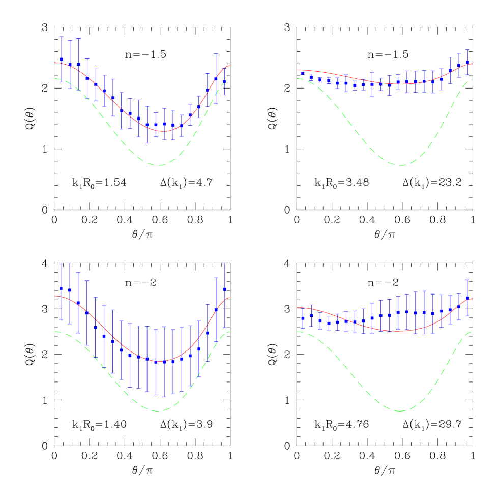
Figure 4: The three-point hierarchical Fourier amplitude $Q_{3}$ for configurations with $k_{1}/k_{2}=2$ as a function of the angle $\theta$ between ${\hbox{\BF k}}_{1}$ and ${\hbox{\BF k}}_{2}$, at different scales for $n=-1.5$ (top) and $n=-2$ (bottom) scale-free initial conditions. Symbols denote measurements in numerical simulations (taken from Scoccimarro et al. (1998), Figs. 1, 2, and 3). The solid curves show the bispectrum fitting formula, Eqs. (16) to (20). The dashed curves correspond to the predictions of tree-level PT.

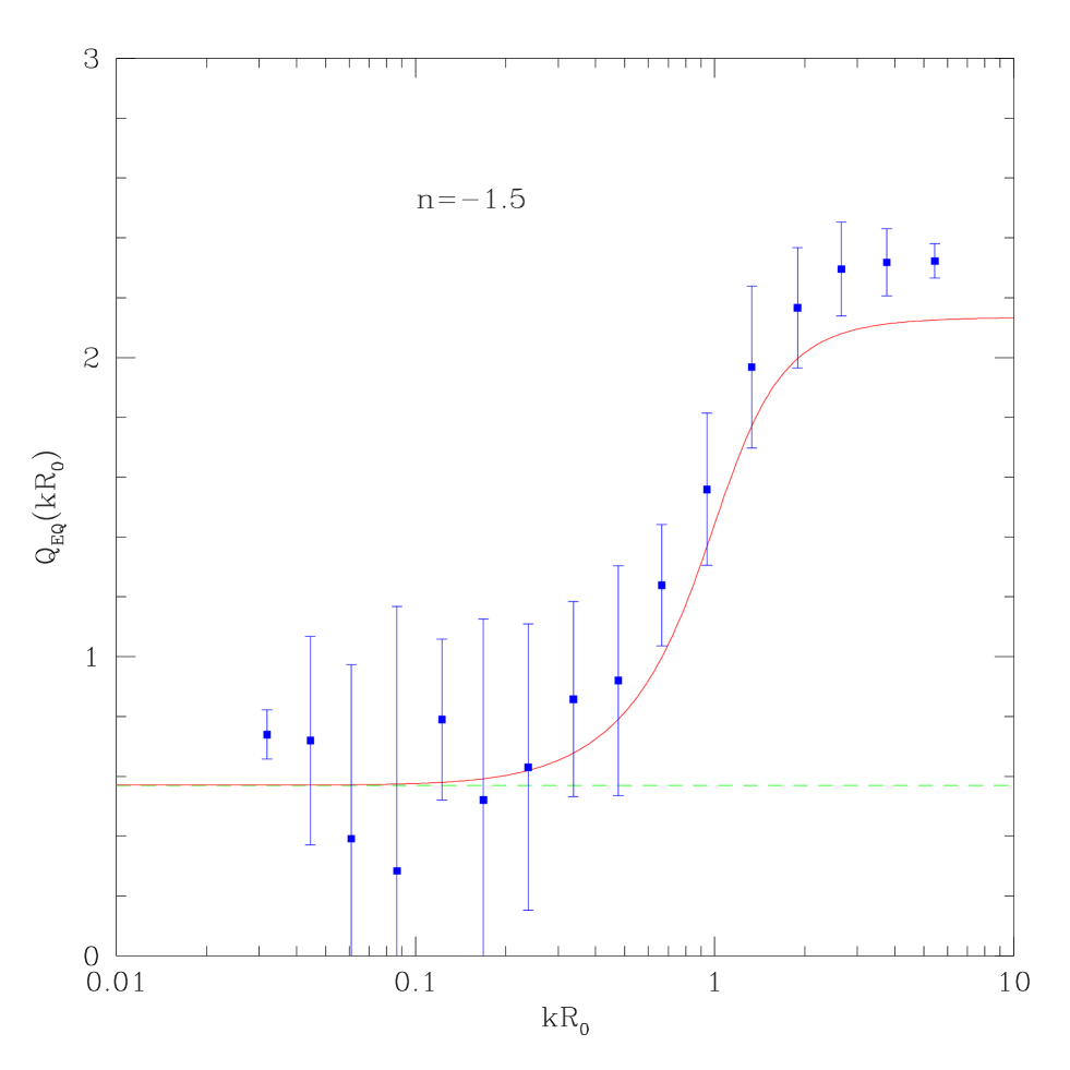
Figure 5: The three-point hierarchical Fourier amplitude $Q_{\rm EQ}$ for equilateral triangle configurations and $n=-1.5$ scale-free initial conditions as a function of scale. Symbols denote measurements in numerical simulations (taken from Scoccimarro et al. (1998), Fig. 9). The solid curve shows the bispectrum fitting formula, Eqs. (16) to (20), and the dashed line corresponds to the prediction of tree-level PT, $Q_{\rm EQ}=4/7$.

Figure 4 shows the fitting formula for the hierarchical three-point amplitude $Q_{3}$ (solid curves) as a function of angle $\theta$ between ${\hbox{\BF k}}_{1}$ and ${\hbox{\BF k}}_{2}$ for configurations with $k_{1}/k_{2}=2$ configurations. These configurations are studied at different scales characterized by the value of $k_{1}R_{0}$. The power spectrum amplitude $\Delta(k)=4\pi k^{3}P(k)$ provides a measure of the degree of non-linearity on these scales. The numerical simulation measurements shown here are taken from Figs. 1, 2, and 3 of SCFFHM. These N-body results correspond to $256^{3}$ PM simulations run by E. Hivon; the bispectrum measurements were done by S. Colombi, according to the scheme outlined in Appendix A of SCFFHM. In order to obtain $Q_{3}$ from Eq. (16) we have used Eq. (8) and used the linear power spectrum $P(k)\propto k^{n}$; due to cancellations between the numerator and denominator, using the non-linear power spectrum (e.g., as given by Peacock & Dodds (1996)) does not change $Q_{3}$ appreciably, though it does affect the bispectrum itself. Figure 5 shows a plot of the evolution of the equilateral hierarchical amplitude $Q_{\rm EQ}$ as a function of scale for $n=-1.5$ scale-free initial conditions. The results in Figs. 4 and 5 were found to be typical of the accuracy of the fitting formula, which is of order $15\%$ for the scale-free models considered in SCFFHM. Generalization of Eqs. (18)-(20) to CDM spectra is under way and will be reported elsewhere.

Note that at intermediate scales, the functions $a(n,k)$, $b(n,k)$, and $c(n,k)$ in Eq. (17) break the scale invariance of $Q$, as required in the one-loop regime. We have chosen the overall scale dependence to be separable, in order to simplify applications of the fitting formula to large-scale structure calculations. For example, the skewness may be interpolated by

$$S_{3}(R)=\frac{30}{7}\ \frac{\sigma_{a}^{4}}{\sigma^{4}}+\frac{4}{7}\ \frac{\sigma_{c}^{4}}{\sigma^{4}}-\frac{\sigma_{b}^{4}}{\sigma^{4}}\ (n+3),$$ (21)

where

$$\sigma_{j}^{2}(R)\equiv\int d^{3}k\ P(k)\ j(n,k)\ W^{2}(kR),$$ (22)

for $j=a,b,c$. In this way, only straightforward one-dimensional numerical integrations are required to calculate $S_{3}$ at any scale $R$, using, e.g., the non-linear power spectrum from Peacock & Dodds (1996). Figure 6 shows an application of this result for $n=-1$ scale-free initial conditions (solid curve), compared to numerical simulation measurements by CBH. Different symbols denote different expansion factors, $a=2.5$ (triangles), $a=6.4$ (squares), and $a=16$ (pentagons), where initial conditions were set at $a=1$. Error bars, not shown for clarity, are of the order of $20\%$ (CBH); thus the results of Eq. (21) are well within the N-body uncertainties. It seems, however, that the fit in Eq. (21) lies consistently above the N-body results. This is to be expected, at least up to $\sigma^{2}\approx 1$, since the numerical simulation measurements are affected by transients from the Zel’dovich approximation used to set up the initial conditions (Scoccimarro 1998). In fact, for the $a=2.5$ output (triangles) in Fig. 6, the $\sigma^{2}\rightarrow 0$ limit including transients corresponds to $S_{3}=2.39$ instead of the tree-level PT value $S_{3}=2.86$ shown by the dashed line.

5 Conclusion

We have proposed a simple ansatz, called Hyperextended Perturbation Theory (HEPT), to calculate clustering amplitudes, such as the hierarchical $S_{p}$ parameters, in the strongly non-linear regime. Based on N-body studies of scale-free and CDM models, the HEPT ansatz appears to be valid for all initial conditions of physical interest and has the advantage that it contains no free parameters. The proposal is based on extrapolating tree-level PT to the non-linear regime by using configurations that correspond to matter flowing parallel to density gradients.

The similarity between the hierarchy of tree-level and strongly non-linear $S_{p}$ parameters was pointed out by Colombi et al. (1997), who noticed that by using the tree-level expressions for the $S_{p}$ with an arbitrary spectral index they could fit the whole hierarchy of $S_{p}$ parameters in the non-linear regime. However, no explanation for such a remarkable coincidence was given. Within the HEPT framework, this arises naturally as a consequence of identifying the most important configurations that drive gravitational collapse. This provides a valuable tool for quantitative understanding of the behavior of higher-order correlations in the non-linear regime, based on simple physics borrowed from perturbation theory. At the same time, we caution that these results are only meant to provide insight into non-linear gravitational clustering: in the real universe, the clustering of luminous galaxies on these scales will be strongly affected by non-gravitational phenomena as well, such as gas dissipation, star formation, shocks, etc.

We have also provided a fitting formula for the evolution of the bispectrum in scale-free models from the weakly to the strongly non-linear regime. This expression interpolates between the perturbative results on large scales and the saturation behavior observed in simulations at small scales. This result should be useful for applications in large-scale structure calculations. For example, using our results to obtain the skewness $S_{3}$ as a function of scale and initial spectrum, one can implement the EPT framework of Colombi et al. (1997) to predict the rest of the one-point cumulants, $S_{p}$, for $p>3$ at any scale.

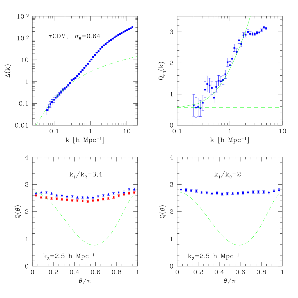
Figure 1: The upper left panel shows the power spectrum, $\Delta(k)=4\pi k^{3}P(k)$, for the $\tau$CDM model ($\sigma_{8}=0.64$). Other panels show the hierarchical three-point Fourier amplitude $Q_{3}$ for equilateral triangles (top right) and for configurations with different $k_{1}/k_{2}$ ratios (bottom) in the non-linear regime (in the lower left, triangles correspond to $k_{1}/k_{2}=3$, squares to $k_{1}/k_{2}=4$). Dashed curves show the predictions of tree-level PT. The solid curve in upper right panel shows the prediction of one-loop PT.

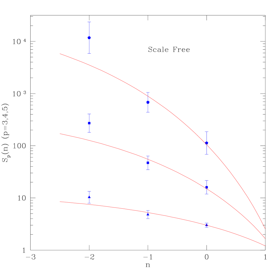
Figure 2: The hierarchical $S_{p}$ parameters: skewness (triangles, $p=3$), kurtosis (squares, $p=4$), and pentosis (pentagons, $p=5$) are shown for scale-free initial conditions in numerical simulations by Colombi, Bouchet & Hernquist (1996). The solid curves denote the predictions of HEPT, Eqs. (12), (13), and (14).

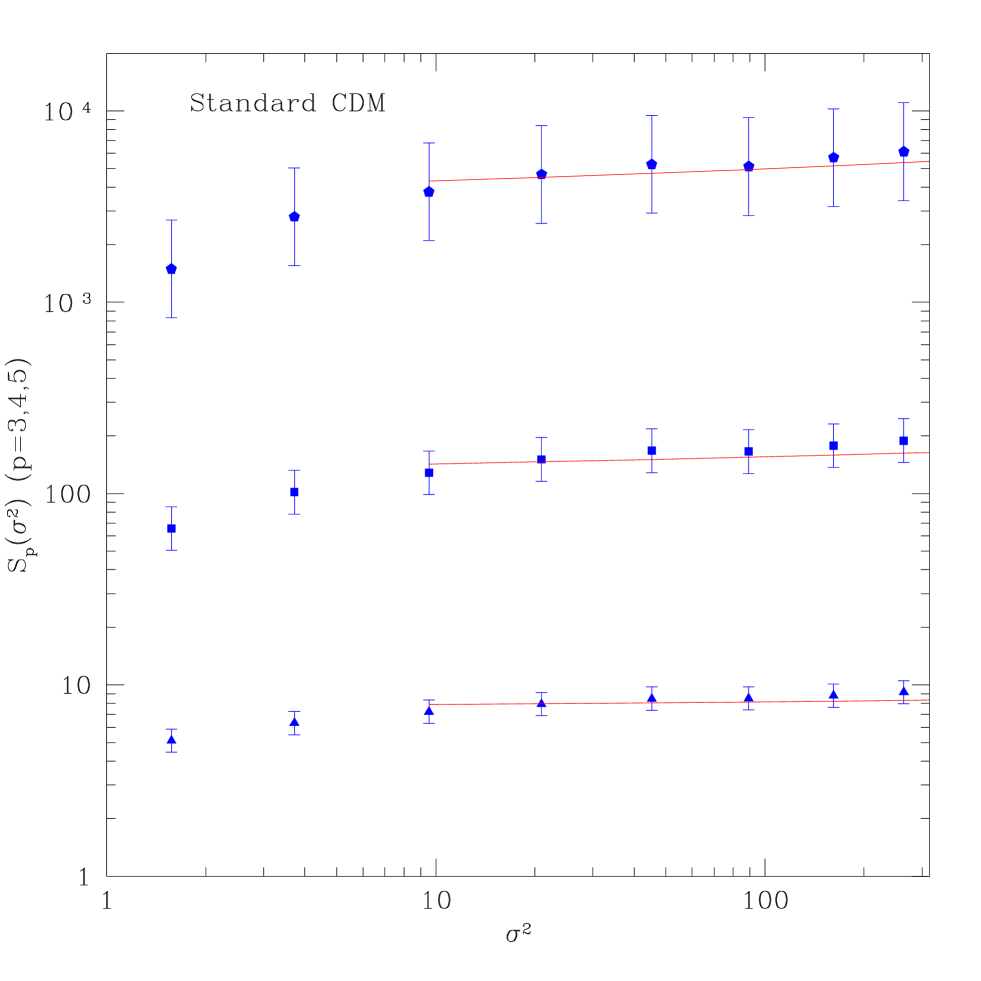
Figure 3: The skewness (triangles), kurtosis (squares), and pentosis (pentagons) parameters for the standard CDM spectrum ($\sigma_{8}=0.34$) from numerical simulations by Colombi, Bouchet, & Schaeffer (1994). The solid curves denote the predictions of HEPT, Eqs. (12), (13) and (14).

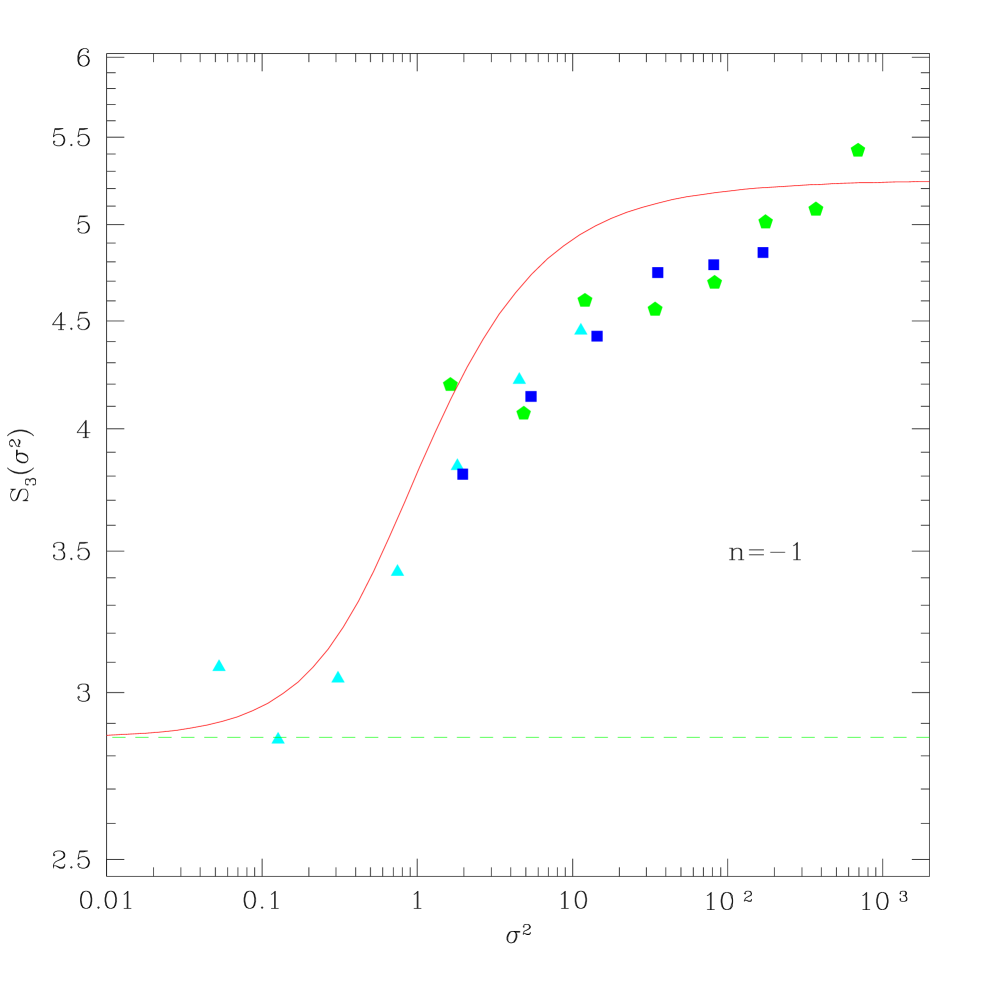
Figure 6: Predictions of our fitting formula for the skewness $S_{3}$ for $n=-1$ scale-free initial conditions as a function of the variance $\sigma^{2}$ for top-hat smoothing. Different symbols denote numerical simulation measurements at different expansion factors, $a=2.5$ (triangles), $a=6.4$ (squares), and $a=16$ (pentagons), where initial conditions were set at $a=1$. Error bars, not shown to avoid clutter, are of the order of $20\%$ (Colombi, Bouchet, & Hernquist (1996)). The solid curve shows the fitting formula of Eq. (21), and the dashed line corresponds to the prediction of tree-level PT, $S_{3}=20/7$. The systematic underestimate of N-body results is likely due to transients from initial conditions (see text).