Topological lens effects in Universes with Non-Euclidean Compact Spatial Sections

Abstract

Universe models with compact spatial sections smaller than the observable universe produce a topological lens effect. Given a catalog of cosmic sources, we estimate the number of topological images in locally hyperbolic and locally elliptic spaces, as a function of the cosmological parameters, of the volume of the spatial sections and of the catalog depth. Next we apply the crystallographic method, aimed to detect a topological signal in the 3D distance histogram between images, to compact hyperbolic models. Numerical calculations in the Weeks manifold allows us to check the absence of crystallographic signature of topology, due to the fact that the number of copies of the fundamental domain in the observable covering space is low and that the points are not moved the same distance by the holonomies of space.

]

I Introduction

The question of whether our universe has a finite spatial extension or not is still an open question related to the topology of the universe (see [1] for a review and [2] for latest developpements). Recently, there has been a large activity to constrain and/or to observe the shape and the size of the universe. Many methods have been proposed to detect its spatial topology using catalogs of discrete sources (clusters of galaxies [3], quasars[4]) and the cosmic microwave background[5, 6, 7, 8]. All the methods rest on a “topological lens” effect which generates multiple images of cosmic sources, as soon as the compact spatial sections have a volume smaller than the observable universe. In the past, the idea of using the topological images was extensively applied to universe models with Euclidean (see e.g. [9, 10, 11, 12]) and hyperbolic (see e.g. [13]) spatial sections . More recently, the crystallographic method [3], which relies on the existence of topological images whatever the underlying geometry, was applied only to locally flat universes, and was able to put a bound on the characteristic size $L$ of Euclidean space to $L\leq 650\,h^{-1}\hbox{Mpc}$ (with $h=H_{0}/100\,\hbox{km/s/Mpc}$, $H_{0}$ being the Hubble constant). The efficiency of the crystallographic method obviously depends on the number of topological images of a given object within the horizon size or within the limits of current catalogs used for the test. The applicability of the method in Euclidean space has also been discussed by Fagundes and Gausmann [14] when the size of the physical space is comparable to the horizon size.

We can naturally wonder if the method applies as well in locally hyperbolic or elliptic manifolds, and if we can get any constraint on the size of space from the existing catalogs of cosmic objects. We keep also in mind the growing weight of observational evidence for a low density universe (see e.g. Spergel in [2]). Thus in this article we focus mainly on universes with locally hyperbolic compact spatial sections [15]. The universe is described by a 4-manifold ${\cal M}$ and a Lorentzian metric ${\bf g}$ and we assume that ${\cal M}$ can be splitted as ${\cal M}=\Sigma\times R$ (see e.g. [16] for the conditions of such a splitting). As any multi-connected closed three-dimensional manifold, $\Sigma$ can be described by its fundamental domain (a polyhedron) and its holonomy group $\Gamma$, which identifies the faces of the polyhedron by pairs [1]. Such hyperbolic manifolds $\Sigma=H^{3}/\Gamma$ have a remarkable property that links topology and geometry : the rigidity theorem [17, 18] implies that geometrical quantities such as the volume, the lengths of its closed geodesics, …, are topological invariants. The volume of the manifold can then be used to classify these manifolds [15]. The volumes of compact hyperbolic manifolds are bounded below [19] by:

$$\hbox{Vol}(\Sigma)\geq\hbox{Vol}_{\rm min}\simeq 0.166,$$ (1)

in units of the curvature radius.

The smallest known compact hyperbolic manifold, likely to produce the greatest topological lens effects, is the Weeks space [20, 21] (see Appendix A for a description), such that

$$\hbox{Vol}=0.94272,\quad r_{+}=0.7525,\quad r_{-}=0.5192,$$ (2)

where $r_{+}$ and $r_{-}$ are respectively the radii of the largest (smallest) geodesic ball that contains (is contained in) the fundamental domain.

The fundamental domain and the holonomy group of the known three–dimensional compact hyperbolic manifolds can be found by using the software SnapPea [22] which gives all the informations needed to compute the topological lens effects, such as the volume, the generators of the holonomy group, the lengths of closed geodesics.

Fagundes [23] already used a universe whose spatial sections had the topology of the Weeks manifold to discuss the controversy about the quasars redshifts. In his paper, he gave an interesting description of the fundamental domain and of the holonomy group. The same author previously studied a 2+1 hyperbolic cosmology [24] and a universe with hyperbolic spatial sections whose fundamental domain was a hyperbolic icosahedron [25] (known as the Best space [26]) to investigate the same problem.

In section II we describe the crystallographic method and the way to implement it, focusing on the interface with SnapPea. In §III, we discuss the applicability of this method in compact hyperbolic universes (§III A) and in compact elliptic universes (§III B) and specially the dependence of the number of images in function of the density parameter and of the cosmological constant. We then give (§IV) the numerical results of simulations in the Weeks manifold, and discuss the influence of the catalog, of the density parameter and of the position of the observer within the fundamental domain.

II The crystallographic method in compact hyperbolic universes

In this section, we describe the crystallographic method and the way to implement it to universes with compact hyperbolic spatial sections. The local geometry of such a universe is described by a Friedmann-Lemaître metric

$$ds^{2}=-dt^{2}+a^{2}(t)\left(d\chi^{2}+\sinh^{2}{\chi}d\Omega^{2}\right).$$ (3)

where $a$ is the scale factor, $t$ the cosmic time and $d\Omega^{2}\equiv d\theta^{2}+\sin^{2}{\theta}d\varphi^{2}$ the infinitesimal solid angle.

A locally hyperbolic three–dimensional manifold can be embedded in four–dimensional Minkowski space by introducing the set of coordinates $(x^{\mu})_{\mu=0..3}$ related to the intrinsic coordinates $(\chi,\theta,\varphi)$ through (see e.g. [28, 29])

$$x_{0} = \cosh{\chi}$$ (4)

$$x_{1} = \sinh{\chi}\sin{\theta}\sin{\varphi}$$ (5)

$$x_{2} = \sinh{\chi}\sin{\theta}\cos{\varphi}$$ (6)

$$x_{3} = \sinh{\chi}\cos{\theta},$$ (7)

so that the three–dimensional hyperboloid $H^{3}$ has the equation

$$-x_{0}^{2}+x_{1}^{2}+x_{2}^{2}+x_{3}^{2}=-1.$$ (8)

[Note that when $a(t)=t$, the line element (3) describes a Milne universe which, using the coordinates transformation $(t^{\prime}=t\cosh\chi,r=t\sinh\chi)$ reduces to the Minkowski line element in spherical coordinates. This can describe a $\Omega=0$ open cosmology (see e.g. [27]).]

With these notations, the comoving spatial distance between two points of comoving coordinates $x$ and $y$ can be computed directly in the Minkowski space by [25]

$$d[x,y]=\arg\cosh{\left[\frac{x^{\mu}y_{\mu}}{\left(x^{\mu}x_{\mu}\right)^{1/2}\left(y^{\mu}y_{\mu}\right)^{1/2}}\right]},$$ (9)

where $x_{\mu}=\eta_{\mu\nu}x^{\nu}$, $\eta_{\mu\nu}$ being the Minkowskian metric. Note that Minkowski space can be mapped onto the interior of an ordinary sphere $S^{2}$ of unit radius by using the Klein coordinates $(X_{i})_{i=1..3}$ [28, 29] defined by

$$X_{i}=x_{i}/x_{0}.$$ (10)

The universal covering space being described, we now choose a topology, i.e. a holonomy group $\Gamma$ such that the spatial sections are ${\Sigma}=H^{3}/\Gamma$. ${\Sigma}$ can be described by its fundamental domain whose $2K$ faces are identified by pairs by the elements of $\Gamma$. $\Gamma$ has $2K$ generators which, in the case of the Weeks manifold ($K=9$) can be obtained from SnapPea and are given in appendix A.

Indeed, the elements of $\Gamma$ are isometries so that

$$\forall x,y\in\Sigma\quad\forall g\in\Gamma,\quad\hbox{dist}[x,y]=\hbox{dist}[g(x),g(y)].$$ (11)

The crystallographic method [3] is based on a property of multi–connected universes according to which each topological image of a given object is linked to each other one by the holonomies of space. Indeed, we do not know these holomies as far as we have not determined the topology, but we know that they are isometries. For instance in locally Euclidean universes, to each holonomy is associated a distance $\lambda$, equal to the length of the translation by which the fundamental domain is moved to produce the tessellation in the covering space. Assume the fundamental domain contains $N$ objects (e.g. galaxy clusters), if we calculate the mutual 3D–distances between every pair of topological images (inside the particle horizon), the distances $\lambda$ will occur $N$ times for each copy of the fundamental domain, and all other distances will be spread in a smooth way between zero and two times the horizon distance. In a histogram plotting the number of pairs versus their 3D separations, the distances $\lambda$ will thus produce peaks. Simulations indeed showed that the pairs between two topological images of the same object drastically emerge from ordinary pairs[3] in the histogram.

Two kind of catalogs of astronomical objects can be thought of to apply this method : the galaxy cluster catalogs, which typically have a redshift depth $z=1$, and the quasars catalogs, which typically extend to $z=3$. Concerning quasars, even if their lifetime is probably too short to be good candidates for producing topological images, they are usually part of systems that have a much larger lifetime [30]. The angular resolution needed is given by the fact that the objects have a peculiar velocity and that they will not be seen at exactly the same position [1]. Note that the crystallographic method, contrary to the “direct” method which would try to recognize topological images of individual objects, is not plagued by the evolution problem, i.e. that topological images of the same object are seen at different stages of its evolution.

III Estimation of the number of topological images in non-Euclidean universes

A Compact hyperbolic universes

To estimate the applicability of the crystallographic method in hyperbolic compact universes, we estimate the number of topological images of a given object up to a redshift $z$. With the metric (3), the Einstein equations reduce to the Friedmann equation

$$H^{2}=\kappa\frac{\rho_{m}}{3}-\frac{K}{a^{2}}+\frac{\Lambda}{3},$$ (12)

$\rho_{m}$ being the matter density, $\Lambda$ the cosmological constant and $\kappa\equiv 8\pi G/c^{4}$. $H$ is the Hubble constant defined by $H\equiv\dot{a}/a$ with $\dot{X}\equiv\partial_{t}X$. We choose the units such that the curvature index is $K=-1$. Introducing $\Omega_{\Lambda}\equiv\Lambda/3H^{2}$, $\Omega_{m}\equiv\kappa\rho_{m}/3H^{2}$ and the redshift $z$ defined by $1+z\equiv a_{0}/a$, (12) can be rewritten as (see e.g. [31])

$$\frac{H^{2}}{H_{0}^{2}}=\Omega_{m0}(1+z)^{3}+\Omega_{\Lambda 0}+(1-\Omega_{m0}-\Omega_{\Lambda 0})(1+z)^{2}.$$ (13)

For that purpose we have used equation (12) evaluated today (i.e. at $t=t_{0}$) and we have assumed that we were in a matter dominated universe so that $\rho_{m}\propto a^{-3}$ [this hypothesis is very good since we restrict ourselves to small redshift].

The radius of the observable region at a redshift $z$ is given by integration of the radial null geodesic equation $d\chi=dt/a$ and reads

$$\chi(z) \equiv \int_{a_{0}}^{a}\frac{da}{a\dot{a}}$$ (14)

$$= \int_{\frac{1}{1+z}}^{1}\frac{\sqrt{1-\Omega_{m0}-\Omega_{\Lambda 0}}dx}{x\sqrt{\Omega_{\Lambda 0}x^{2}+(1-\Omega_{m0}-\Omega_{\Lambda 0})+\frac{\Omega_{m0}}{x}}}.$$ (15)

(15) is integrated numerically and the result can be compared, when $\Omega_{\Lambda}=0$, to the analytic expression (see e.g. [32])

$$\chi(z)=\left[\arg\cosh{\left(1+\frac{2(1-\Omega_{m0})}{\Omega_{m0}}x\right)}\right]^{1}_{\frac{1}{1+z}}.$$ (16)

The number of topological images of a given object at a redshift $z$ can be estimated by computing the ratio between the volume of the geodesic sphere of radius $\chi(z)$ and the volume of the manifold which is a topological invariant. This leads to

$$N(\Omega_{m0},\Omega_{\Lambda 0};z<Z)=\frac{\pi\left(\sinh{2\chi(Z)}-2\chi(Z)\right)}{\hbox{Vol}(\Sigma)}.$$ (17)

It can be easily understood that this under-estimates the number of images.

As seen on figure 1, detecting the topology with clusters of galaxies would require both $\Omega_{\Lambda 0}$ and $\Omega_{m0}$ to be very low. The situation is much better with groups of quasars (figure 2). Figure 3 shows the effect of the two parameters ($\Omega_{\Lambda}$,$\Omega_{m}$) on the number of topological images inside the observable universe. This also provides an estimation of the number of expected matched circles in the circle method [7].

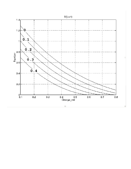
FIG. 1.: Number of topological images in a catalog of clusters up to a redshift $z=1$ in function of $\Omega_{m0}$ and $\Omega_{\Lambda 0}$ in a universe whose spatial sections have the topology of the Weeks manifold. The curves are labeled by the values of $\Omega_{\Lambda 0}$. Topology is detectable only if the number of topological images is greater than unity.

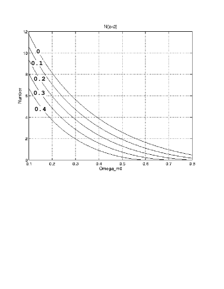
FIG. 2.: The same as Figure 1 in the case of a catalog of quasars extending up to a redshift $z=3$.

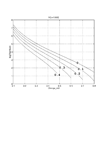
FIG. 3.: Number of topological images within the observable universe (i.e. with $z<1000$) in function of $\Omega_{m0}$ and $\Omega_{\Lambda 0}$. This estimates the number of expected matched circles on the cosmic microwave background.

Given standard values of the cosmological parameters [33], the numbers of pairs involving an object and one of its topological images will be statistically low in compact hyperbolic universes. For instance a cluster catalog will give no signature whatever the parameters and a quasar catalog will typically require the cosmological constant to vanish and the density parameter to be $\Omega_{m0}<0.4$. It can also be seen that the generic effect of the cosmological constant is to make the horizon volume bigger and thus to dilute the number of topological images.

B compact elliptic universes

We proceed as in the previous section but now the spatial sections are of the form $S^{3}/\Gamma$, where the holonomy group $\Gamma$ is either a cyclic group, a dihedral group or the symmetry groups $T,O,I$ respectively of the tetrahedron, octahedron or isocahedron (see [1] for a complete description). The local geometry of the background spacetime is described by a Friedmann-Lemaître universe with the metric

$$ds^{2}=-dt^{2}+a^{2}(t)\left(d\chi^{2}+\sin^{2}{\chi}d\Omega^{2}\right).$$ (18)

In units of the curvature radius (i.e. when $K=+1$), the volume of the spatial sections is given by

$$\hbox{Vol}(S^{3}/\Gamma)=\frac{\hbox{Vol}(S^{3})}{|\Gamma|}=\frac{2\pi^{2}}{|\Gamma|},$$ (19)

where $|\Gamma|$ is the order of the group $\Gamma$ (e.g. $|\Gamma|=12,24,60$ respectively for $T,O,I$) [1, 28]. Since the volume of the sphere of radius $\chi$ is given by

$$\hbox{Vol}(\chi)=\frac{2\chi-\sin{2\chi}}{2\pi},$$ (20)

the number of topological images defined as in §III A, is

$$N(\Omega_{m0},\Omega_{\Lambda 0};z<Z)=\frac{|\Gamma|}{2\pi}\left(2\chi(Z)-\sin{2\chi(Z)}\right).$$ (21)

$\chi(Z)$ is computed as in equation (13-15) by changing the sign of the curvature index $K$ in (12) [note that it does not affect equation (13)] so that

$$\chi(z)=\int_{\frac{1}{1+z}}^{1}\frac{\sqrt{\Omega_{m0}+\Omega_{\Lambda 0}-1}dx}{x\sqrt{\Omega_{\Lambda 0}x^{2}+(1-\Omega_{m0}-\Omega_{\Lambda 0})+\frac{\Omega_{m0}}{x}}}.$$ (22)

When $\Omega_{\Lambda}=0$, this expression can be computed analytically, as in equation (16) [31]

We plot $N/|\Gamma|$ in term of $\Omega_{m0}$ for different values of $\Omega_{\Lambda 0}$. It can be concluded that the topology of an elliptic space can be detected respectively by a catalog of galaxy clusters (see figure 4) only if $|\Gamma|>200$ and if $|\Gamma|>50$ in a catalog of quasars (see figure 5) when $\Omega_{\Lambda}=0$.

A non vanishing cosmological constant improves the situation and holonomy groups of lower order can be considered. Nevertheless, we are still constrained by the fact that the total energy density has to be compatible with the estimated age of the universe.

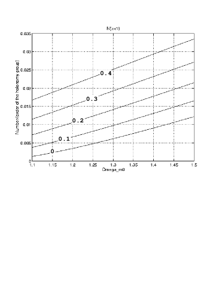
FIG. 4.: Number of topological images in a galaxy cluster catalog up to a redshift $z=1$ in function of $\Omega_{m0}$ and $\Omega_{\Lambda 0}$ in a locally elliptic space.

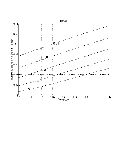
FIG. 5.: Same as figure 4 for a catalog of quasars up to a redshift $z=3$.

IV Numerical results

In our numerical simulations, we concentrate only on compact hyperbolic models. We first generate an idealised catalog, ${\cal C}$, by distributing homogeneously objects in the fundamental domain. A homogeneous distribution is defined by the requirement that the number of objects per unit volume is constant, i.e. by

$$\frac{dN}{dV}=constant,$$ (23)

$dV$ being given by

$$dV = \sinh^{2}{\chi}d\chi\sin\theta d\theta d\varphi$$ (24)

$$= d[\cosh{2\chi}-2\chi]d\cos{\theta}d\varphi,$$ (25)

with $\cos{\theta}\in[-1,1]$ and $\varphi\in[-\pi,\pi]$. We first create a catalog in the smallest sphere containing the fundamental polyhedron. Then, in order to obtain a set ${\cal C}_{1}$, we reject the points lying outside the fundamental domain by checking if they are on the same side of the faces of the fundamental domain than its center. This can easily be achieved when we know the Minkowskian coordinates of the vertices of the polyhedron, which can be obtained from SnapPea (see Appendix A).

We then unfold the catalog by applying the generators of the holonomy group to obtain the set ${\cal C}_{2}$

$${\cal C}_{2}=\left\{\tilde{x},\forall x\in{\cal C}_{1},\quad\tilde{x}=\sum_{g\in\Gamma}g(x);\quad\chi(\tilde{x})\leq\chi_{m}\right\},$$ (26)

where $\chi_{m}$ is the maximal value of the radial coordinate of the set ${\cal C}_{2}$. To generate a catalog with a given depth $z$ in redshift, we truncate ${\cal C}_{2}$ so that

$${\cal C}(z)=\left\{x\in{\cal C}_{2};\quad\hbox{dist}[0,x]\leq\chi(\Omega_{m0},\Omega_{\Lambda 0};z)\right\},$$ (27)

where $\chi(\Omega_{m0},\Omega_{\Lambda 0};z)$ is given by equation (15). This accounts as selecting the objects located within the geodesic ball of radius $\chi(\Omega_{m0},\Omega_{\Lambda 0};z)$ centered onto an observer placed at the centre.

We then compute all the three dimensional separations between all the pairs of ${\cal C}(z)$ and plot the histogram of the number of pairs with a given separation.

Indeed the former procedure applies when the observer stands at the center of the polyhedron $(\chi=0)$. Now, if the observer is at a position, $(\chi_{\oplus}\not=0,\theta_{\oplus}=0,\varphi_{\oplus}=0)$ say, we have to perform a coordinate change to “center” the catalog on the observer before selecting the object as in (27). The Minkowskian coordinates, $x^{\prime}$ say, of a point in the frame centered on the observer are related to the “old” coordinates $x$ (i.e in the frame centered on $\chi=0$) by

$$x^{\prime}={\cal M}_{0\rightarrow\oplus}x\quad{\rm with}\quad{\rm det}({\cal M}_{0\rightarrow\oplus})=1,$$ (28)

where ${\cal M}_{0\rightarrow\oplus}$ is a matrix determined by the fact that the image of the “old” center $\chi=0$ is the observer’s position $x_{\oplus}=(\cosh{\chi_{\oplus}}\equiv\gamma,0,0,\sinh{\chi_{\oplus}}\equiv\beta\gamma)$ so that

$${\cal M}_{0\rightarrow\oplus}=\left(\begin{array}[]{cccc}\gamma&0&0&-\beta\gamma\\ 0&1&0&0\\ 0&0&1&0\\ -\beta\gamma&0&0&\gamma\end{array}\right).$$ (29)

We recognize a Lorentz transformation. The same method applies when $\theta_{\oplus}\not=0$ and $\varphi_{\oplus}\not=0$ but the matrices are not so straightforward, so that we do not consider them here.

The catalog ${\cal C}(z)$ is then constructed as in (27) but using the points ${x^{\prime}}$ instead of $x$, and the procedure of pair computation is not affected.

We now generate some pair histograms in a universe whose spatial sections have the topology of the Weeks manifold using $N=1000$ objects in the fundamental domain. In figure (6) we assume that $\Omega_{\Lambda}=0$, $\Omega_{m0}=0.2$, that the observer stands at the center of the polyhedron ($\chi=0$) and that he uses a galaxy cluster catalog of depth $z=1$. We then study the dependence on $\Omega_{m0}$ (see figure 7 where $\Omega_{m0}=0.5$), on the position of the observer (see figure 8 where the observer stands near a face) and on the catalog depth (see figure 9 where we assume that the observer is using a quasar catalog of depth $z=3$).

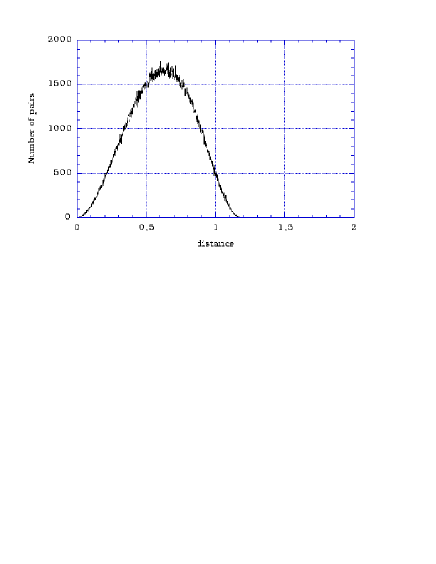
FIG. 6.: Pair histogram for a galaxy cluster catalog ($z=1$) measured by an observer centered in $\chi=0$ in a hyperbolic universe whose spatial sections have the topology of the Weeks manifold and $\Omega_{m0}=0.2$; $\Omega_{\Lambda}=0$.

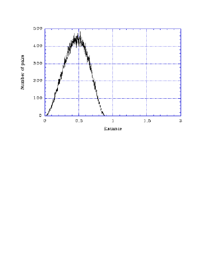
FIG. 7.: Pair histogram for a galaxy cluster catalog ($z=1$) measured by an observer centered in $\chi=0$ in an universe whose spatial sections have the topology of the Weeks manifold and $\Omega_{m0}=0.5$.

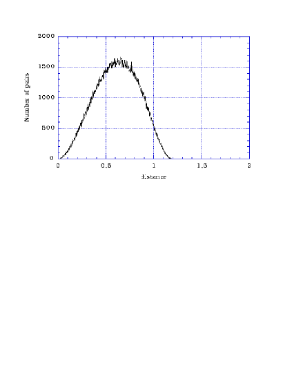
FIG. 8.: Pair histogram for a galaxy cluster catalog ($z=1$) measured by an observer located near a face of the Weeks fundamental domain. Its Klein coordinates are $x=(0,0,\tanh{0.5})$ and $\Omega_{m0}=0.2$.

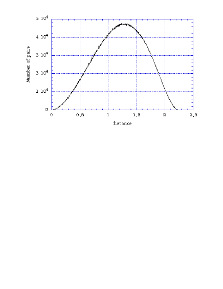
FIG. 9.: Pair histogram for a quasar catalog ($z=3$) measured by an observer centered in $\chi=0$ in an universe whose spatial sections have the topology of the Weeks manifold and $\Omega_{m0}=0.2$.

As a matter of fact, we do not observe any peaks in these histograms, contrarily to the case of locally Euclidean universes. Let us try to understand why. Two kinds of pairs can give birth to peaks (see figure 10):

1. Type I pairs of the form $\{g(x),g(y)\}$, since $\hbox{dist}[g(x),g(y)]=\hbox{dist}[x,y]$ for all points and all elements $g$ of $\Gamma$.

2. Type II pairs of the form $\{x,g(x)\}$ if $\hbox{dist}[x,g(x)]=\hbox{dist}[y,g(y)]$ for at least some points and elements $g$ of $\Gamma$.

Type I pairs are always present, whatever the topology. Their number roughly equals the number of copies of the fundamental domain within the catalog’s limits. Type II pairs produce peaks when the separation distance between topological images is independent of the location of the source.

In compact locally Euclidean universes, type I and type II pairs are both present. The reason is that the 3-torus has the very special property that the separation distance of gg-pairs (i.e. any pair of images comprising an original and one of its ghosts, or two ghosts of the same object) is independent of the location of the source. In other Euclidean spaces the spectrum of gg-pair distances varies with the location of the source. However all closed Euclidean 3-manifolds have the 3-torus as a covering space, so for each such manifold there will be some distances which are independent of the location of the source. As a consequence, the topological signal expected in the histogram from type I and type II pairs clearly stands out, as was shown in the simulations of [3].

In compact hyperbolic manifolds, $\hbox{dist}[x,g(x)]$ always depends on the position $x$ of the source [15]. This fact is clearly illustrated by the numerical calculation of figure 11. Thus type II pairs cannot appear (see figure 10). Moreover, as shown in §III A, the number of type I pairs is too low to generate significant peaks in the distance histogram. Hence the crystallographic method fails.

The small number of Type I pairs in hyperbolic manifolds is due to the property that the volume of the manifold is fixed once the topology is determined (the rigidity theorem) contrary to Euclidean spaces where the characteristic sizes and the volume of the fundamental polyhedron can be choosen at will (since $K=0$ the geometry does not impose any characteristic size).

In elliptic spaces, distances are position-independent whenever the holonomy is a Clifford translation [34]. A Clifford translation is an isometry $g$ such that the displacement function $\hbox{dist}(x,g(x))$ is constant. This is precisely what is required to get type II pairs in the histogram. All finite groups of Clifford translations of spheres are the cyclic group, the binary dihedral, tetrahedral, octahedral and icosahedral groups [28]. Next (theorem 7.6.7 in [28]): $S^{3}/\Gamma$ is a Riemannian homogeneous elliptic space if and only if $\Gamma$ is a group of Clifford translations of $S^{3}$. Given the classification of three–dimensional spherical space forms (see [1], §7), we deduce that all homogeneous elliptic spaces usable for cosmology, such as lens spaces $L(p)=S^{3}/Z_{p}$ or the Poincaré dodecahedral space, satisfy this property. The covering transformations which take a source to its nearest neighbours are Clifford translations (although the transformations to more distant neighbours might not be), and type II pairs can be produced.

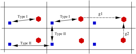
FIG. 10.: The difference between type I and type II pairs on the example of the two dimensional torus (the translations $g_{1}$, $g_{2}$ $g_{1}^{-1}$ and $g_{2}^{-1}$ are the generators of its holonomy group). Type I pairs are the ones between the ghosts of two distinct objects and type II pairs are the ones between two topological images of the same object (hexagon or square).

FIG. 11.: The function $\hbox{dist}[x,g_{1}(x)]$ for all the points located within the fundamental domain of Weeks manifold and on the disk ${\varphi=0}$ for the generator $g_{1}$ given in Appendix A. This illustrates the fact that this function depends on $x$ in a locally hyperbolic manifold, contrary to Euclidean manifolds.

V conclusion

In this article, we generalised the crystallographic method based on the existence of topological images, to universes with non-Euclidean compact spatial sections.

The analysis was performed by using the smallest known compact hyperbolic manifold, where we expect to have the greatest number of topological images. It turns out that we do not observe, contrary to Euclidean universes, any peaks in the pair 3D separation histogram.

The absence of peaks is due to combined effects, of the mathematics and of the cosmological parameters.

1. Locally hyperbolic manifolds are such that $\hbox{dist}[x,g_{n}(x)]$ depends on $x$, so that there is no amplification for the type II pairs $\{x,g_{n}(x)\}$, whereas $\hbox{dist}[x,g_{n}(x)]=\hbox{dist}[y,g_{n}(y)]$ in the Euclidean case. This suppresses the peaks.

2. The peaks associated to the isometries (i.e. such that $\forall g\in\Gamma,\quad\hbox{dist}[g(x),g(y)]=\hbox{dist}[x,y]$) must remain. But, given the cosmological parameters, we have shown in §III A that the number of topological images is too low to create such peaks associated to type I pairs.

In elliptic universes, we have studied the influence of the cosmological parameters. As in the hyperbolic case, type I pairs can be observed for very small universes only and, as in the Euclidean case, type II pairs may be present, due to the fact that the holonomies are Clifford translations. However, such universes are not favored by the present estimates of the cosmological parameters [33].

We conclude that in practice, the crystallographic method will be able to detect the topology only if the universe is locally Euclidean. Such universes have the interesting property that the characteristic sizes of their fundamental domain are decoupled from the cosmological parameters and thus from the Hubble radius. Whatever the underlying geometry, discrete sources such as quasars, X-ray galaxy clusters or infrared galaxies can still help to investigate the cosmic topology by looking for multiple images of individual objects.

Acknolewdgments

We are grateful to J. Weeks and H. Fagundes for their precious comments.

Appendix A : Description of the Weeks manifold

We considered the Weeks manifold [closed census m003(-3,1)]. Its fundamental polyhedron has 18 faces and 26 vertices (see figure 12). All the following quantities are needed to perform our computation and can be obtained from the software SnapPea. The volume of the manifold, in units of the curvature radius, is $0.94272$.

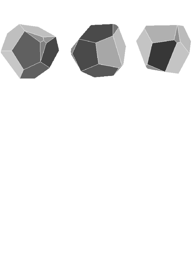
FIG. 12.: Three views of the fundamental domain of the Weeks manifold.

The Klein coordinates (10) of the 26 vertices are

label	$X_{1}\quad\,$	$X_{2}\quad\,$	$X_{3}\quad\,$
0	0.10797407	0.34689848	-0.41772745
1	-0.00056561	-0.36314169	-0.51501423
2	0.03670097	-0.29313316	-0.54565764
3	-0.08402116	-0.35849225	-0.49943971
4	-0.23493634	0.01568564	-0.59147636
5	-0.08019087	0.60971881	0.08263574
6	0.00049690	0.31902895	0.45245272
7	-0.42135580	-0.01132323	0.46844736
8	-0.44370265	0.45474638	-0.04023802
9	-0.03061224	0.62921121	0.01637099
10	-0.06244403	0.61432068	-0.06105007
11	0.52204774	0.13760656	-0.30585432
12	-0.51128589	0.15380739	-0.31614284
13	-0.50817234	-0.21892234	-0.01808485
14	0.04566464	-0.41129238	-0.46235223
15	-0.18945313	-0.58387452	-0.16877044
16	-0.34964269	0.00034506	0.51260720
17	-0.43363513	-0.08848249	0.43491114
18	-0.11977854	-0.34363564	0.52235338
19	-0.01122014	-0.58564972	0.20470658
20	0.56409719	0.28438251	0.07878044
21	0.43096130	0.11398724	0.43161967
22	0.45298033	0.03203520	0.43691467
23	0.49689789	-0.00018511	0.37162982
24	0.39981755	-0.37241380	0.08914633
25	0.42311163	-0.25223127	-0.40328816

The 18 faces are then defined by their vertices as

faces	Number of	label of	label of	label of	label of	label of
	vertices	vertex 1	vertex 2	vertex 3	vertex 4	vertex 5
I	5	23	24	25	11	20
II	5	2	4	0	11	25
III	5	22	18	19	24	23
IV	5	10	0	4	12	8
V	5	8	7	16	6	5
VI	5	15	13	12	4	3
VII	5	17	13	15	19	18
VIII	5	14	25	24	19	15
IX	5	18	22	21	6	16
X	5	9	20	11	0	10
XI	5	7	8	12	13	17
XII	5	5	6	21	20	9
XIII	4	3	4	2	1
XIV	4	20	21	22	23
XV	4	7	17	18	16
XVI	4	1	2	25	14
XVII	4	1	14	15	3
XVIII	4	10	8	5	9

The 18 generators of the holonomy group can then be written as

$$g_{1}=\left(\begin{array}[]{rrrr}1.58926252069783&-0.40490373463745&-0.18520828837947&1.15217455938197\\ 1.19813100468664&-0.37867518857251&-0.43845341527127&1.44909682512520\\ -0.29994054013040&0.58749594014885&-0.79530849910863&-0.33510780230833\\ -0.01652657525663&0.82182763167926&0.45776096815586&0.33959883323000\end{array}\right)$$

$$g_{2}=\left(\begin{array}[]{rrrr}1.58926252069784&0.58852165407720&-0.78772550995989&-0.74758688012532\\ 0.60542090101752&0.63256516975419&-0.95802870162689&0.22040140712305\\ -0.74661392026174&-0.95121865744570&0.02947692798603&0.80730819540762\\ 0.77575031187707&-0.20347508215704&-0.83774912510678&-0.92658666119331\end{array}\right)$$

$$g_{3}=\left(\begin{array}[]{rrrr}1.58926252069784&0.90966168251236&0.52649891309985&0.64889897331428\\ -0.39527310953786&-0.96583883836601&-0.09504624064542&0.46299285260867\\ 0.83783613378036&0.46865953388686&1.11407913829435&0.49107565810403\\ -0.81703435760262&-0.82158259245920&0.16430152540933&-0.98262515437950\end{array}\right)$$

$$g_{4}=\left(\begin{array}[]{rrrr}1.58926252069784&-0.50251081201258&1.10144921603985&0.24504666492427\\ -0.80335677967765&0.05959497029949&-0.93768098628153&-0.87326108520599\\ -0.85819691489983&0.41642334058451&-1.15485297933977&0.47896570051526\\ 0.37930370351109&-1.03709071788392&0.01610402406107&0.26087315458913\end{array}\right)$$

$$g_{5}=\left(\begin{array}[]{rrrr}1.58926252069784&-0.11125231907787&-0.10906253703873&-1.22535041690502\\ 0.61314085066332&-0.72730066360826&-0.62733910551353&-0.67336549819589\\ 0.97779233966538&0.49501806133898&-0.13277443919182&-1.30130931248255\\ -0.44015428821540&0.48822939502184&-0.77505563153628&0.59553053934699\end{array}\right)$$

$$g_{6}=\left(\begin{array}[]{rrrr}1.58926252069784&-0.48013536446388&-0.94330313872012&-0.63671389176518\\ -1.21801166215147&0.63453136165388&1.27966469214643&0.66586833224629\\ 0.12199830361655&0.75940754853765&-0.15821652454111&-0.64276845961162\\ 0.16528570559051&-0.50119865773022&0.47670391078232&-0.74085940056587\end{array}\right)$$

$$g_{7}=\left(\begin{array}[]{rrrr}2.07713761580105&-1.55800356296413&-0.47129628725962&-0.81547862165852\\ -0.34790844003080&0.59158539050820&-0.84366445697397&0.24351035382656\\ -0.55790510170459&0.95617333032507&0.27707820937007&-0.56587837100861\\ -1.69770500671437&1.47075980034853&0.65846650660136&1.13379440781211\end{array}\right)$$

$$g_{8}=\left(\begin{array}[]{rrrr}2.07713761580106&-0.62403517630796&0.95362111998219&1.41974910925485\\ -0.85113707827869&0.92242574522307&0.12808289744563&-0.92582927257265\\ -0.52567197801091&-0.52156865254264&0.00566611122130&-1.00213026315664\\ 1.52109674922046&-0.51625263825403&1.37584734147421&1.07436615124600\end{array}\right)$$

$$g_{9}=\left(\begin{array}[]{rrrr}2.07713761580107&0.70433686017330&-1.67848312773007&0.03323631000097\\ -0.28072927025369&0.14834866484720&0.42816244471325&0.93460072638127\\ -1.44346161316703&-0.14613011383240&1.71843229305311&-0.33048127437171\\ -1.07336402171483&-1.20529211233965&0.82521087317360&0.13567704979006\end{array}\right)$$

The nine other matrices are defined by $g_{k+9}=g_{k}^{-1}$ and any element $g\in\Gamma$ can be written as

$$g=\prod_{i\in I}g_{n_{i}};\qquad n_{i}\in\{1,..,18\}.$$

REFERENCES

- [1] M. Lachièze-Rey and J.-P. Luminet, Phys. Rep. 254, 135 (1995).
- [2] Proceedings of the workshop Cosmology and topology, Cleveland 25-27 october 1997, Class. Quant. Grav. 15(1998).
- [3] R. Lehoucq, M. Lachièze-Rey and J-P. Luminet, Astron. Astrophys. 313, 339 (1996).
- [4] B.F. Roukema, Month. Not. R. Astron. Soc. 283, 1147 (1996); B.F. Roukema and A.C. Edge, Month. Not. R. Astron. Soc. 292, 105 (1997).
- [5] D. Stevens, D. Scott and J. Silk, Phys. Rev. Lett. 71, 20 (1993).
- [6] A. de Oliveira Costa, G.F. Smoot and A.A. Starobinsky, Astrophys. J. 468, 457 (1996).
- [7] N.J. Cornish, D.N. Spergel and G.D. Starkman, Phys. Rev. D57, 5982 (1998); ibid., Proc.Nat.Acad.Sci. 95, 82 (1998); ibid. Class. Quant. Grav. 15, (1998).
- [8] J.P. Uzan, Phys. Rev. D58, 087301 (1998); ibid., Class. Quant. Grav. 15, 2711 (1998).
- [9] L.Z. Fang and H. Sato, Comm. Theoret. Phys. (China) 2, 1055 (1983).
- [10] M. Demianski and M. Lapucha, Month. Not. R. Astron. Soc. 224, 527 (1987).
- [11] H.V. Fagundes and W.F. Wichoski, Astrophys. J. 322, L5 (1987).
- [12] G.F.R. Ellis, Gen. Rel. Grav. 2, 7 (1971).
- [13] J.R. Gott III, Month. Not. R. Astron. Soc. 193, 153 (1980).
- [14] H.V. Fagundes and E. Gaussman, astro-ph/9704259
- [15] W.P. Thurston, The topology and geometry of three manifolds, Princeton Lecture Note (1979); Three Dimensional Geometry and Topology, ed. S. Levy, Princeton University Press (1997).
- [16] S. Hawking and G.F.R. Ellis Large scale structure of spacetime, Cambridge university Press (1973).
- [17] G.D. Mostow, Ann. Math. Studies 78, Princeton University Press (1973).
- [18] G. Prasad, Invent. Math. 21, 255 (1973).
- [19] D. Gabai, G.R. Meyerhoff and N. Thurston, MSRI preprint 1996-058 (1996).
- [20] J. Weeks, PhD Thesis, Princeton University (1985).
- [21] S.V. Matveev and A.T. Fomenko, Russian Math. Surveys 43, 3 (1988).
- [22] J. Weeks : http://www.geom.umn.edu:80/software.
- [23] H.V. Fagundes, Phys. Rev. Lett. 70, 1579 (1993).
- [24] H.V. Fagundes, Astrophys. J. 291, 450 (1985).
- [25] H.V. Fagundes, Astrophys. J. 338, 618 (1989); Astrophys. J. 349, 678 (1960).
- [26] L.A. Best, Canadian J. Math. 23, 451 (1971).
- [27] C.W. Misner, K.S. Thorne and J.A. Wheeler, Gravitation, San Francisco, Freeman (1973).
- [28] J.A. Wolf, Spaces of constant curvature, fifth edition, Publish or Perish Inc., Wilmington USA (1984).
- [29] H.S.M. Coxeter, Non Euclidean geometry, University of Toronto Press (1965).
- [30] G. Paál, Acta. Phys. Acad. Hungaricae 30, 51 (1971).
- [31] P.J.E Peebles, Principles of Physical Cosmology, Princeton University Press (1993).
- [32] I.S. Gradstheyn and I.M. Ryzhik, Table of integrals series and products, ed. Academic N.Y. (1980).
- [33] Proceedings of the “XXIIIrd rencontres de Moriond : Fundamental Parameters in Cosmology”, Eds. Trân Thanh Vân (1998).
- [34] J. Weeks, private communication.