The influence of geometry and topology on axisymmetric mean-field dynamos

Abstract

We study the changes in the dynamical behaviour of axisymmetric spherical mean-field dynamo models produced by changes in their geometry and topology, by considering a two parameter family of models, ranging from a full sphere to spherical shell, torus and disc–like configurations, within a unified framework. We find that the two parameter space of the family of models considered here separates into at least three different regions with distinct characteristics for the onset of dynamo action. In two of these regions, the most easily excited fields are oscillatory, in one case with dipolar symmetry, and in the other with quadrupolar, whereas in the third region the most easily excited field is steady and quadrupolar. In the nonlinear regime, we find that topological changes can alter significantly the dynamical behaviour, whilst modest changes in geometry can produce qualitative changes, particularly for thin disc–like configurations. This is of potential importance, since the exact shapes of astrophysical bodies, especially accretion discs and galaxies, are usually not precisely known.

1 Introduction

The magnetic fields observed in stars, accretion discs and galaxies are generally considered to be generated by magnetohydrodynamic dynamo action. The complexity of the physics of such dynamos has meant that a fully self-consistent model is beyond the range of the computational resources currently available, although important attempts have been made to understand turbulent dynamos in stars (Nordlund et al. 1992, Brandenburg et al. 1996) and accretion discs (Brandenburg et al. 1995, Hawley et al. 1996), for example. Such studies have had to be restricted to the geometry of a Cartesian box, thus they are in essence local dynamos. However, magnetic fields in astrophysical objects are observed to exhibit large scale structure, related to the shape of the object, and thus can only be captured fully by global dynamo models. In some cases it has been possible to show that, for fully three-dimensional turbulence simulations, the dependence of the results (parity, time dependence, cycle period, etc.) on global properties including boundary conditions is remarkably similar to that of the corresponding mean-field dynamo models (Brandenburg 1999). This lends some support to the validity of mean-field theory, which is used in the following.

Mean field dynamo models, which attempt to capture such geometric features, have been employed extensively in order to study various aspects of the dynamics of solar, stellar and galactic dynamos (see for example, Steenbeck & Krause 1969, Roberts & Stix 1972). Often the dimensionality of the underlying partial differential equations has been reduced by assuming axisymmetry. As the presence of strong differential rotation tends to destroy non-axisymmetric fields (e.g. Rädler 1986), this restriction has some astrophysical justification, but nevertheless some galaxies and types of stars are known to have non-axisymmetric fields and so this simplification cannot be universally valid.

In addition to producing solutions with pure and mixed parities (Brandenburg et al. 1989a,b), these studies have also revealed new features such as solutions with both chaotic behaviour (see for example Jones et al. 1985 in a severely truncated system, Brooke & Moss 1994, Torkelsson & Brandenburg 1994b, Tavakol et al. 1995) and intermittent modes of behaviour (see e.g. Brooke & Moss 1995; Tobias & Weiss, 1997; Tworkowski et al. 1998, Covas et al. 1998a).

An important shortcoming of these models is that they involve severe approximations, which essentially fall into two broad categories. There are those concerning the underlying physics, such as approximations involved in the parameterisation of the turbulent processes in solar and stellar convective zones (which are not known precisely), and there are the simplifications assumed in modelling the phenomenological features of these systems, such as the details of their geometries. These shortcomings are often ignored, the assumption being that changing the details of these models should not change their behaviours qualitatively. A priori, however, there are no reasons why this should be so and it is therefore important that this assumption should be checked.

Recently, an attempt was made to study the robustness of axisymmetric mean-field models in spheres and spherical shells with respect to changes in the functional form of the $\alpha$ effect (Tavakol et al. 1995) and also by considering the $\alpha$–quenching to be dynamic (Covas et al. 1998a). Here we shall employ the usual algebraic $\alpha$–quenching and focus on the second feature discussed above, namely the assumptions regarding the topology and geometry of these models. This is important for two reasons. Firstly, these are the two important features differentiating the astrophysical situations in which such dynamos are thought to be operative. Thus spherical and spherical shell models are considered in connection with solar and stellar variability (with the sphere or shell representing convectively unstable regions of stars), whereas disc (Torkelsson & Brandenburg 1994a,b, 1995) and torus (Brooke & Moss 1994; 1995) models are considered in connection with modelling accretion discs and galaxies. Secondly, the geometries of these models are often only approximations to the true shapes of the astrophysical systems, and so it is important to know the sensitivity of the dynamo solutions to modest changes in geometry. This is particularly true for dynamo models in accretion discs and galaxies.

In this paper we study the qualitative nature of the dynamical behaviour of axisymmetric mean-field dynamo models as a function of changes in their topology, following transitions from sphere to shell to torus, and as a function of changes in their geometry resulting from alteration of the shapes of the dynamo region, whilst retaining the topology. We consider these changes within a unified framework, using the same numerical code with the same boundary conditions, to solve the same dynamo equations. In the context of disc-like models, we also consider changes in the rotation law.

The models considered here include geometric features such as curvature, which are naturally present in astrophysical systems. There have also been studies of more idealized models in Cartesian geometry, and of low order models, which aim to describe generic features of axisymmetric dynamo solutions (e.g. Weiss, Cattaneo & Jones 1984, Jennings et al. 1990, Jennings & Weiss 1991, Jennings 1991, Tobias et al. 1995). It is of interest to determine whether such features persist across changes in geometry and topology and in the highly nonlinear regimes considered here. We shall briefly return to this issue below in the light of our findings.

In section 2 we briefly introduce the equations for the axisymmetric mean-field dynamo models together with the relevant boundary conditions. Section 3 contains a discussion of our results and finally section 4 contains our conclusions.

2 The model

The standard mean-field dynamo equation (cf. Krause & Rädler 1980) is of the form

$$\frac{\partial\@vec{B}}{\partial t}=\nabla\times\left(\@vec{u}\times\@vec{B}+\alpha\@vec{B}-\eta_{t}\nabla\times\@vec{B}\right),$$ (1)

where $\@vec{B}$ and $\@vec{u}$ are the mean magnetic field and the mean velocity respectively. The quantities $\alpha$ (the $\alpha$ effect) and the turbulent magnetic diffusivity, $\eta_{t}$, appear in the process of the parameterisation of the second order correlations between the velocity and magnetic field fluctuations ($\@vec{u}^{\prime}$ and $\@vec{B}^{\prime}$). For the sake of simplicity, and to facilitate comparison with previous work, we shall ignore anisotropies and take $\alpha$ and $\eta_{t}$ to be scalars. We assume that ${\bf u}={\bf\Omega}\times{\bf r}=u_{\phi}\hat{\phi}$. Nondimensionalization of the equations in terms of a length $R$ and a time $R^{2}/\eta_{t}$ produces the two usual dynamo parameters $C_{\alpha}=\alpha_{0}R/\eta_{t}$ and $C_{\omega}=\Omega_{0}R^{2}/\eta_{t}$, where $\alpha_{0}$ and $\Omega_{0}$ are typical values of $\alpha$ and $|{\bf\Omega}|$. For the sake of comparison with existing results (e.g., Covas et al. 1998a), we set $|C_{\omega}|=10^{4}$ throughout (except briefly, in one particular case). We use spherical polar coordinates $(r,\theta,\phi)$ and consider axisymmetric solutions only. In order to satisfy the condition $\nabla\cdot{\bf B}=0$ we solve Eq. (1) by splitting the field into meridional and azimuthal components, ${\bf B}={\bf B}_{p}+{\bf B}_{\phi}$, and expressing these components in terms of scalar field functions, so that ${\bf B}_{p}=\nabla\times a\hat{\mbox{\boldmath$\phi$}}$, ${\bf B}_{\phi}=b\hat{\mbox{\boldmath$\phi$}}$.

We consider the usual algebraic form of $\alpha$–quenching namely

$$\alpha_{a}=\frac{\alpha_{0}\cos\theta}{1+\@vec{B}^{2}},$$ (2)

with $\alpha_{0}={\rm constant}$. This form has been adopted in numerous studies.

In our calculations we consider two types of rotation laws, one with constant shear and the other with approximately rigid rotation close to the rotation axis and tending to Keplerian rotation at larger radii. Hereafter we refer to the latter as a “generalized Keplerian” rotation law. The first constant shear profile has been used extensively in studies in many different geometries. We recognise that helioseismological evidence indicates that the rotational profile of the sun gives a shear in a very concentrated region. Our main aim is to allow comparison with a range of published models, hence we chose this simple and widely used form. The second profile has been extensively used in studies of accretion discs. In that it gives a differential rotation that decreases with radius it might be considered to give a generic representation of the rotation in a galactic disc, although rotation profiles in galaxies are certainly not Keplerian.

For the rotation profiles that we will consider here, we take

$$\@vec{u}=\Omega\varpi\hat{\mbox{\boldmath$\phi$}},$$ (3)

where $\varpi=r\sin\theta$ is the distance from the rotation axis. For the first profile mentioned above, we shall, consistent with Brandenburg et al. (1989a), take $\Omega=\Omega_{0}r$, where $\Omega_{0}$ is constant, and for the second profile, we shall take

$$\Omega=\Omega_{0}\left[1+\left(\frac{\varpi}{\varpi_{0}}\right)^{qn}\right]^{-1/n},$$ (4)

where $q=3/2$ for accretion discs. In conformity with Torkelsson & Brandenburg (1994a), we take $\varpi_{0}$ to be $0.3$ and $n=10$. Relation (4) approximates solid body rotation for small $\varpi$ and approaches Keplerian rotation for $\varpi\gg\varpi_{0}$. Note that for this profile $\partial\Omega/\partial r<0$ when $C_{\omega}>0$, whilst for profile (3) with constant shear the signs are reversed, i.e. $\partial\Omega/\partial r>0$ when $C_{\omega}>0$.

The models we shall consider here are all constructed from a complete sphere of radius $R$. We can remove an inner concentric sphere of radius $r_{0}$ (in order to go smoothly from a sphere to a spherical shell). The change from a sphere or a spherical shell to a torus- or disc-like configuration is produced by excising a cone of semi-angle $\theta_{0}$ about the rotation axis, from the north and south polar regions. The configuration is illustrated in Fig. 1, where the dynamo region is produced by revolving the meridian section shown about the vertical dotted rotation axis through the origin $O$.

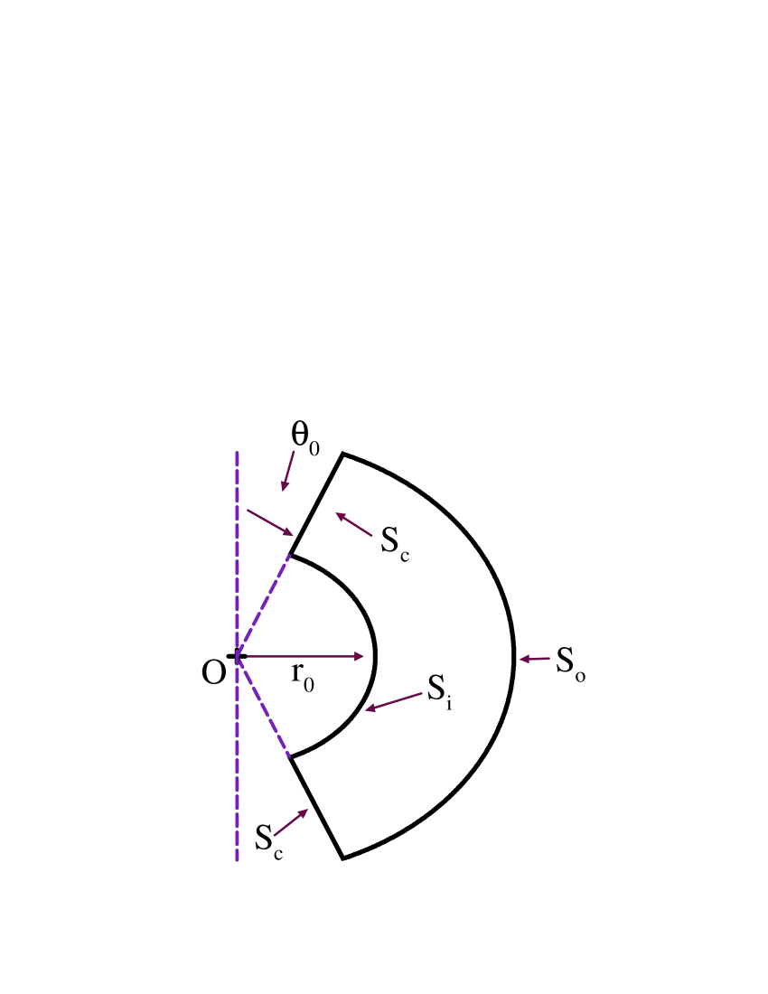
Figure 1: A schematic representation of the dynamo region produced by the cuts characterised by the model parameters $r_{0}$ and $\theta_{0}$.

In order to solve the dynamo equations, boundary conditions need to be imposed on the surfaces of the dynamo region created by removing the cones (denoted by $S_{c}$), on the inner surface $r=r_{0}$ (denoted by $S_{i}$), and also on the outer curved boundary (denoted by $S_{o}$), as depicted in Fig. 1.

We adopt a perfect conductor boundary condition,

$$a=0,\quad{{\partial(rb)}\over{\partial r}}=\alpha{{\partial(ra)}\over{\partial r}}\quad\mbox{on}\quad S_{i}.$$ (5)

Other choices are possible (see, e.g., Tworkowski et al. 1998), but this has been used commonly in earlier investigations.

On $S_{o}$ a vacuum boundary condition has often been used. However this, although appealing, is actually quite arbitrary as, for example, there is no evidence that the solar poloidal field is curl-free immediately above the surface. When $\theta_{0}>0$, implementing an essentially non-local vacuum boundary condition is not straightforward, and so we have chosen a plausible local condition. Other authors have previously taken a radial field condition, $\partial(ar)/\partial r=0$, (e.g. Gilman & Miller 1981). We used

$$\partial a/\partial r=0,b=0,$$ (6)

which results in a poloidal field on $S_{o}$ which is typically near to radial over most of the boundary. We stress that, in the absence of a detailed model of processes above a stellar surface, all choices of boundary condition on $S_{o}$ are more-or-less arbitrary, within general restrictions of plausibility.

If a perfect conductor boundary condition is used on the surfaces $S_{c}$ then as $\theta_{0}\rightarrow 0$ the model does not tend to that used for the full sphere, where $a=b=0$ on the axis. Thus we set

$$a=b=0\quad\mbox{on}\quad S_{c},$$ (7)

to ensure continuity of behaviour as $\theta_{0}\rightarrow 0$; again other choices are possible.

In the following, as is customary, we shall discuss the behaviour of the solutions by monitoring the total magnetic energy, $E={1\over 2\mu_{0}}\int\@vec{B}^{2}dV$, taken over the dynamo region given by $r_{0}\leq r\leq R$ and $\theta_{0}\leq\theta\leq\pi-\theta_{0}$. We split $E$ into two parts, $E=E^{(A)}+E^{(S)}$, where $E^{(A)}$ and $E^{(S)}$ are respectively the energies of those parts of the field whose toroidal field is antisymmetric and symmetric about the equator. The overall parity $P$ is given by $P=[E^{(S)}-E^{(A)}]/E$ (Brandenburg et al. 1989a), so $P=-1$ denotes an antisymmetric (dipole-like) pure parity solution and $P=+1$ a symmetric (quadrupole-like) pure parity solution.

For the numerical results reported in the following sections, we used a modified version of the axisymmetric dynamo code of Brandenburg et al. (1989a). We took a grid size of $41\,\times\,81$ mesh points in the dynamo region. To test the robustness of the code we verified that no qualitative changes were produced by employing a finer grid, different temporal step length (we used a step length of $10^{-4}R^{2}/\eta_{t}$ in the results presented in this paper). We considered a family of models ranging from a full sphere through spherical shells to torus- and disc-like configurations.

3 Results

We present the results of our comparative studies of dynamo solutions in regions that are produced by variations of $r_{0}$ and $\theta_{0}$ in the ranges $0\leq r_{0}<1$ (in dimensionless units) and $0\leq\theta_{0}<\pi/2$ respectively. In particular, we took the following values:

$$r_{0} = 0,\leavevmode\nobreak\ 0.2,\leavevmode\nobreak\ 0.5,\leavevmode\nobreak\ 0.7$$ (8)

$$\theta_{0} = 0,\leavevmode\nobreak\ 4.5^{\circ},\leavevmode\nobreak\ 22.5^{\circ},\leavevmode\nobreak\ 45^{\circ},\leavevmode\nobreak\ 75^{\circ}$$ (9)

To present our results, we use the following notation in the figures: the prefix “steady” denotes a constant energy, whilst “A” and “S” on their own respectively represent pure antisymmetric (dipolar) ($P=-1$) and symmetric (quadrupolar) ($P=+1$) solutions with periodically oscillating energy, “OM” represents solutions which possess periodic oscillations in both parity and energy, and “C” and “I” denote chaotic and intermittent behaviours respectively. By intermittent behaviour we loosely mean irregular switchings between two or more different dynamical regimes characterised by different statistics. (For a precise characterisation of this type of behaviour in some dynamo models see Covas et al. 1998a.) We should add here that the computational cost of our calculations limited the resolution to which we were able to search the parameter space. Consequently all our results regarding the sequence of parity changes are subject to this limitation.

Since many previous authors have discussed behaviour at the onset of dynamo action, we shall present our results in two subsections. First we present our results concerning the onset of dynamo action as we go from a sphere through spherical shells to torus- and disc-like structures, and then we consider the dynamical behaviour for each configuration as the dynamo number is increased. Our detailed results are presented in Table 1 and Figs. 2 to 15.

3.1 The onset of dynamo action

We summarise our onset results by considering the two types of deformation of the basic sphere in turn. Starting with the case where an inner sphere is removed, giving a spherical shell, we note that Roberts (1972) found numerically (but for different boundary conditions) that for an $\alpha\omega$ dynamo with a negative dynamo number, the most easily excited mode has dipole-like symmetry for $r_{0}<0.7$, whereas for $r_{0}\geq 0.7$ the most easily excited mode has quadrupole-like symmetry. Our corresponding results are summarised in Fig. 2. In particular, the top row of this figure, summarizing the behaviour of a sphere and spherical shells without polar cones removed, agrees qualitatively with the results of Roberts (1972).

Figure 2: Schematic representation of the dynamo regions and their corresponding onset parity with $C_{\omega}=-10^{4}$ and a constant rotational shear profile.

Figure 3: Schematic representation of the dynamo regions and their corresponding onset parity. The top and bottom panels are for constant shear and generalized Keplerian rotational profiles respectively.

The next three rows in this figure correspond to the removal of cones of semi-angles $\theta_{0}=4.5^{\circ},22.5^{\circ}$ and $45^{\circ}$ respectively. These results indicate that despite the removal of the polar cones, the onset behaviour still remains the same as that given in Roberts (1972). In this way we may say that the onset results for spheres are quite robust with respect to the polar cuts considered here.

Table 1: Values of $C_{\alpha}$ for the onset of dynamo action as a function of the shell radius $r_{0}$ and the cut angle $\theta_{0}$ with $C_{\omega}=-10^{4}$. The row labeled $*$ is produced using the generalized Keplerian rotation profile given by Eq. (4) with $C_{\omega}=-10^{4}$. Here $SS$ indicates a Steady S state.

$\theta$	$r_{0}=0.0$	$r_{0}=0.2$	$r_{0}=0.5$	$r_{0}=0.7$
$0$	0.45 A	0.38 A	0.31 A	0.42 S
$4.5^{\circ}$	0.45 A	0.38 A	0.32 A	0.42 S
$22.5^{\circ}$	0.70 A	0.60 A	0.42 A	0.50 S
$45^{\circ}$	1.7 A	1.3 A	0.9 A	1.0 S
$48^{\circ}$	1.86 A	1.48 A	1.04 A	1.07 S
$49^{\circ}$	1.98 A	1.58 A	1.10 A	1.113 A
$50^{\circ}$	2.1 A	1.679 A	1.15 A	1.17 A
$55^{\circ}$	3.0 A	2.37 A	1.56 A	1.493 A
$60^{\circ}$	4.45 A	3.545 A	2.27 A	1.98 A
$65^{\circ}$	7.2 A	5.72 A	3.57 A	2.77 A
$67^{\circ}$	9.5 A	7.1 A	4.4 A	3.24 A
$70^{\circ}$	11 SS	8.05 SS	3.09 SS	4.295 A
$75^{\circ}$	13.0 SS	10.1 SS	5.8 SS	7.6 A
$75^{\circ}*$	4.0 SA	3.7 SA	3.5 SA	11.5 SA

To compare our results further with those from in previous studies, for example of dynamo action in tori by Brooke & Moss (1994, 1995) and in discs by Torkelsson & Brandenburg (1994a,b, 1995), we also studied the case of a large polar cut angle ($\theta_{0}=75^{\circ}$), with both constant shear and generalized Keplerian rotation profiles, and these results are summarized in Fig. 3. Note that, as commented after Eq. (4), with the generalized Keplerian rotation law (4), $C_{\omega}>0$ corresponds loosely to the constant shear law with $C_{\omega}<0$. However equal values of $|C_{\omega}|$ do not imply equal values of the rotational shear.

As can be seen from a comparison of Figs. 2 and 3, the onset behaviour in these models changes from oscillatory to steady solutions as the cut angle $\theta_{0}$ increases. Such a change in behaviour has also been found in oblate spheroidal geometry as a sphere flattens to a disc-like configuration (Stix 1975, Soward 1992a,b and Walker & Barenghi 1994). According to these authors, the crucial factor in the change from oscillatory to steady behaviour is the aspect ratio of the spheroids, defined as the ratio of the minor to the major axis. They speculated that this was because dynamo waves were restricted from propagating in the vertical direction (i.e. parallel to the minor axis). In this context it is interesting to note that in our case the only oscillating solution for $\theta_{0}$ = $75^{\circ}$ occurs when $r_{0}=0.7$ and the above aspect ratio is $O(1)$, as for a sphere.

In Table 1 we summarise the values of $C_{\alpha}$ corresponding to the onset of dynamo action in each configuration. Except for the case with generalized Keplerian rotation law, this shows that for a fixed $r_{0}$ the values of $C_{\alpha}$ at the onset of dynamo action increase as the cut angle $\theta_{0}$ increases for almost all configurations as the shells get thicker.

We should also note that the steep increase in the onset value of $C_{\alpha}$, as we go from $\theta_{0}=45^{\circ}$ to $\theta_{0}=75^{\circ}$, may be related to the transition from shell–like to disc–like configurations. Table 1 in conjunction with Figs. 2 and 3 confirm that in the constant shear case configurations with smaller polar cut angles follow the linear results due to Roberts (1972), while those with larger cut angles ($\theta_{0}\ga 49^{\circ}$) do not, thus suggesting the possible existence of a transition as the cut angle is increased.

For the disc–like configurations (with $\theta_{0}\ga 70^{\circ}$), the onset of dynamo action is to a steady state when $r_{0}<0.7$, when the symmetry is determined by the sign of $\frac{\partial\Omega}{\partial r}$. If this is positive, that is for the constant shear with $C_{\omega}=+10^{4}$ and for the generalized Keplerian rotation profile with $C_{\omega}=-10^{4}$, the onset modes are antisymmetric. For the negative case the onset mode is always symmetric.

3.2 Nonlinear regime

We present our results in the nonlinear regime in three stages. First we consider the transition from the full sphere to a spherical shell, then from a full sphere to that with axial cones removed and finally we study a full sphere with both an inner core and axial cones removed simultaneously. Our detailed results are presented in Figs. 4 – 8, corresponding to five different values of $\theta_{0}$. Each contains four panels for each of the values of $r_{0}$ considered, the panels from top to bottom corresponding to $r_{0}$ values of $0.7,0.5,0.2$ and $0.0$ respectively. We have concentrated mostly on the more usual case of negative dynamo number ($C_{\omega}=-10^{4}$), but for comparison we also consider, for large $\theta_{0}$, the case of a positive dynamo number ($C_{\omega}=+10^{4}$; see Fig. 9), as well as the case with generalized Keplerian differential rotation, which is relevant for accretion discs (Figs. 10–12).

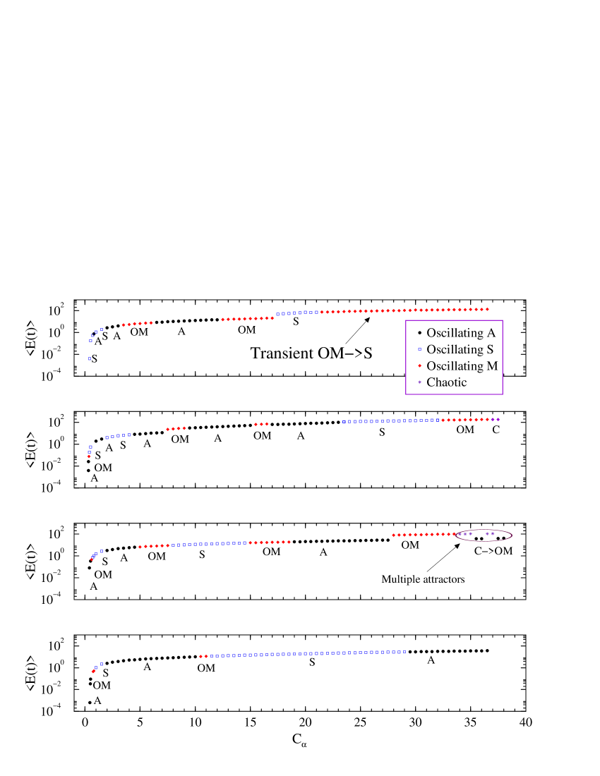
Figure 4: Partial bifurcation diagram, showing the energy in the stable solution, for the case of complete spherical shells ($\theta_{0}=0$), with constant (negative) shear, $C_{\omega}=-10^{4}$. For oscillatory modes, the mean energy is plotted. Here and in following figures, the panels from top to bottom correspond to $r_{0}$ values $0.7,0.5,0.2$ and $0.0$ respectively.

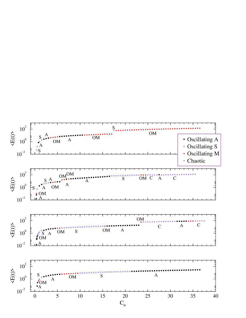
Figure 5: Partial bifurcation diagram, as Fig. 4, for the case of a polar cut with a very small angle $\theta_{0}=4.5^{\circ}$ and with constant (negative) shear, $C_{\omega}=-10^{4}$.

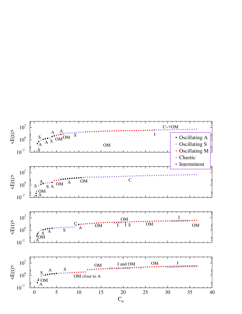
Figure 6: Partial bifurcation diagram, as Fig. 4, for the case $\theta_{0}=22.5^{\circ}$ with constant (negative) shear, $C_{\omega}=-10^{4}$.

Before discussing our results in detail we emphasise that the sequence of parity changes reported below are those that we found to within the resolution of the $C_{\alpha}$ parameter employed here. It is therefore important to bear in mind that unless there is a clear theoretical reason for believing in the presence of a particular sequence of parity changes in the nonlinear regimes, it is always possible to miss finer details of such sequences for any given finite resolution in $C_{\alpha}$. Our standard step in $C_{\alpha}$ is 0.5, but on occasion this was very much reduced (see, e.g., Fig. 13). In addition, although we have attempted to integrate over times long enough to eliminate any transient effects, nonetheless, it is not possible to always rule out the presence of very long-lived transients. With these qualifications we proceed to discuss our results in more detail.

The results concerning the transition from a full sphere to spherical shells are shown in Fig. 4. This shows that the transitions, from the onset of dynamo action into the nonlinear regimes as $C_{\alpha}$ increases, are the same for the full sphere and the two thickest shells (i.e. $r_{0}=0.0,0.2,0.5$). All possess the same initial sequence of parity changes given by

$$A,OM,S,A.$$ (10)

The only difference is that, as the shells become thinner ($r_{0}$ increases), the sequence is compressed to a narrower interval of $C_{\alpha}$. For the thinnest shell ($r_{0}=0.7$), however, the initial sequence is

$$S,A,S,A.$$ (11)

When a polar cone is removed ($\theta_{0}>0$), the initial sequence of parity changes is the same for the full sphere and the two thickest shells for $\theta_{0}\leq 45^{\circ}$. The behaviour for the thinnest shell ($r_{0}=0.7$) and the largest polar cut angle ($\theta_{0}=75^{\circ}$) differ. We also observe that the removal of the polar cones causes more changeable and varied behaviour, as does the removal of the inner cores, providing that the first bifurcation is to an oscillating solution.

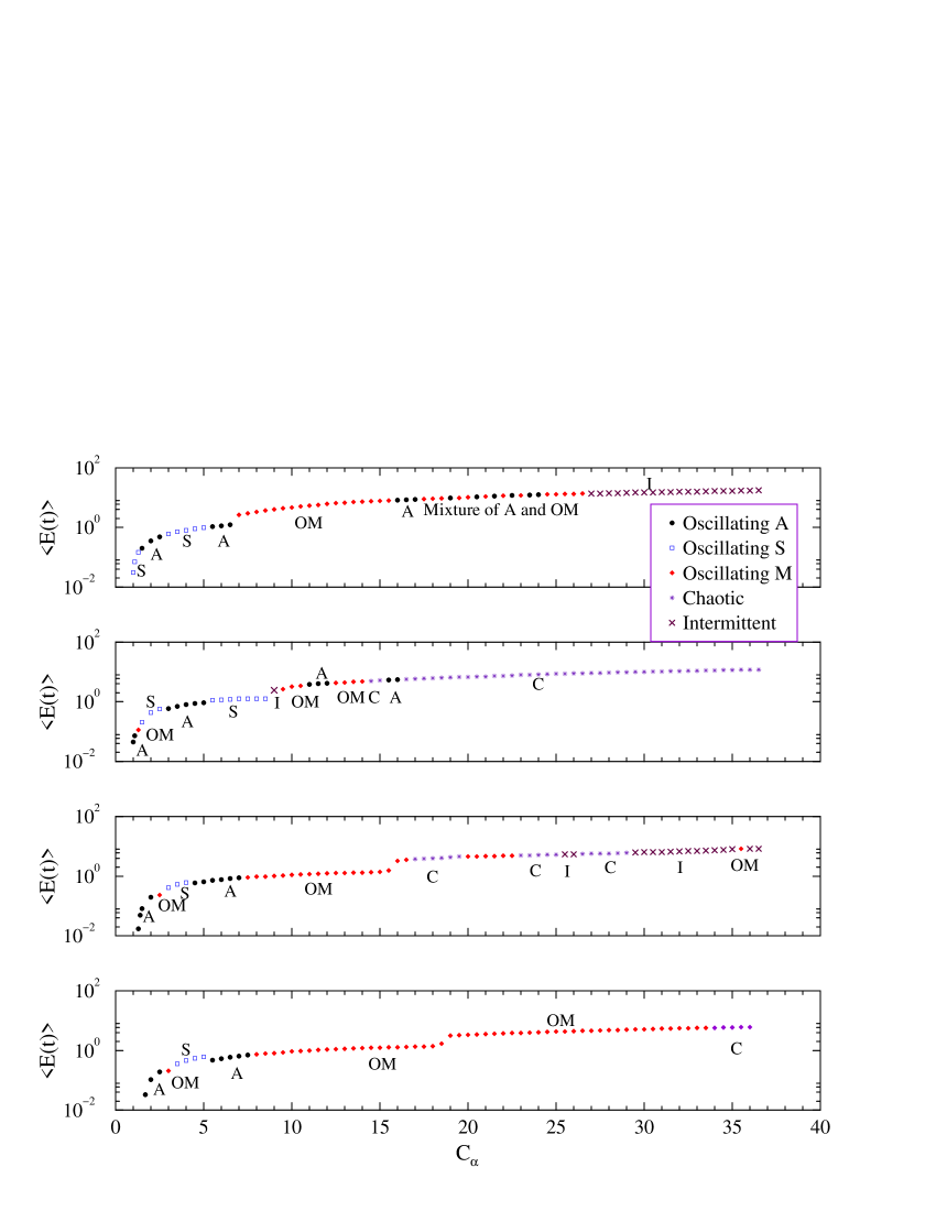
Figure 7: Partial bifurcation diagram, as Fig. 4, for the case $\theta_{0}=45^{\circ}$, with constant (negative) shear, $C_{\omega}=-10^{4}$.

Figures 5 to 7 show that there are similarities in the initial sequences of parity changes as $\theta_{0}$ changes. The configurations with $\theta_{0}=4.5^{\circ},22.5^{\circ}$ and $45^{\circ}$ and $r_{0}=0.0,0.2$ and $0.5$ all have the same initial sequence, namely,

$$A,OM,S,A,$$ (12)

whilst configurations with $r_{0}=0.7$ and these same angles have the sequence

$$S,A,S,A.$$ (13)

These two initial sequences agree with the corresponding ones in the full sphere case ($\theta_{0}=0^{\circ}$). Differences in the bifurcation sequences tend to appear at larger values of $C_{\alpha}$ where the dynamo becomes more non–linear. Also at these higher values of $C_{\alpha}$, more exotic behaviours such as intermittency and chaos can appear, for example for $\theta_{0}=0^{\circ}$ and $4.5^{\circ}$ with $r_{0}=0.2$ and $0.5$, $\theta_{0}=22.5^{\circ}$ with $r_{0}=0.2,0.5$ and $0.7$, and $\theta_{0}=45^{\circ}$ for all values of $r_{0}$ considered here, whilst chaotic and intermittent behaviour only occurs for $\theta_{0}=75^{\circ}$ when $r_{0}=0.7$.

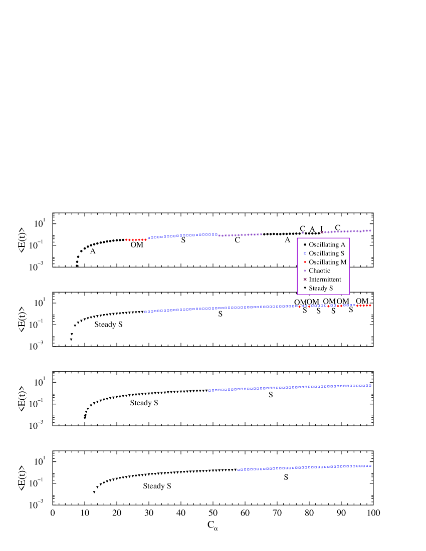
Figure 8: Partial bifurcation diagram, as Fig. 4, for the case of a large polar cut angle, $\theta_{0}=75^{\circ}$, with constant (negative) shear, $C_{\omega}=-10^{4}$.

When $\theta_{0}=75^{\circ}$ (Fig. 8) the behaviour is totally different. The steady quadrupole mode ($S$) remains stable for a very large range of values of $C_{\alpha}$. At some point an oscillatory $S$ mode takes over. For $r_{0}=0.5$ $OM$ modes appear and only for $r_{0}=0.7$ are oscillatory modes observed for all values of $C_{\alpha}$ studied.

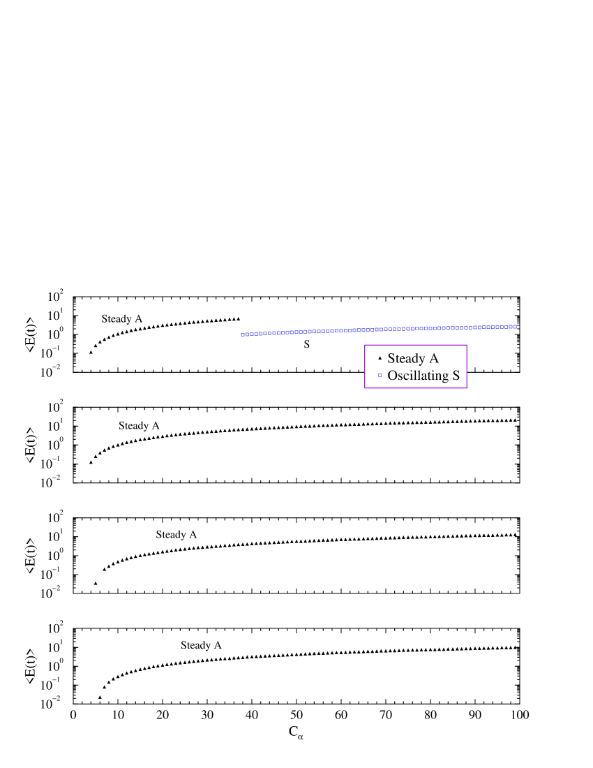
Figure 9: Partial bifurcation diagram, as Fig. 4, for the case of a large polar cut angle, $\theta_{0}=75^{\circ}$, with constant (positive) shear, $C_{\omega}=+10^{4}$.

We also studied the effects of changing the sign of $C_{\omega}$ on our results and this is shown in Fig. 9. As can be seen, a steady $A$ mode is first excited for all $r_{0}$. The general behaviour is also less complex and more uniform, particularly if we compare the panel corresponding to $r_{0}=0.7$ for both signs of $C_{\omega}$.

The effects of changing the rotation law to the generalized Keplerian rotation law are depicted in Fig. 10 and, as can be seen, the steady $S$ mode and the subsequent oscillatory $S$ mode are stable for all values of $C_{\alpha}$ considered. Only in the case $r_{0}=0.7$ is new behaviour seen, in that there is an interval ($C_{\alpha}\approx 15$) where only the trivial solution with zero magnetic field exists. Such a gap in the bifurcation diagram has been found earlier in connection with torus and accretion disc dynamos (e.g. Brooke & Moss 1995, Torkelsson & Brandenburg 1994b, see also Ruzmaikin et al. 1980 and Stepinski & Levy 1991 for linear results). Immediately after this gap an antisymmetric mode appears. The existence of this gap does not appear to be a peculiarity associated with the particular value of $C_{\omega}$ we used, as we also found it when $C_{\omega}=2.7\times 10^{4}$, a value chosen to give the same value of the rotational shear at the mean radius of the shell ($r=0.85$) as the constant shear model with $C_{\omega}=-10^{4}$, shown in Fig. 8. We show these results in Fig. 11. It is clear from comparing Fig. 10 and Fig. 11 that the bifurcation sequence is sensitive to the value of $C_{\omega}$, but the gap in which no field is excited remains.

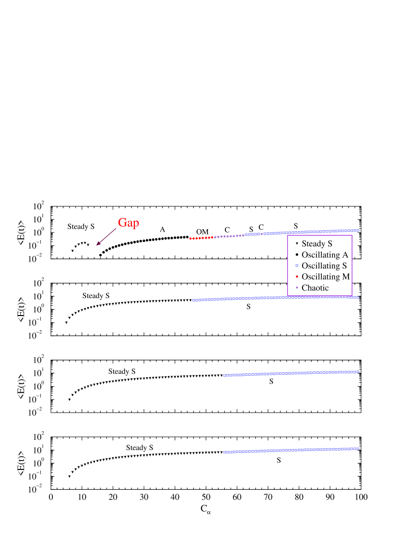
Figure 10: Partial bifurcation diagram, as Fig. 4, for the case of a large polar cut angle, $\theta_{0}=75^{\circ}$, with the generalized Keplerian rotation law, $C_{\omega}=+10^{4}$ ($\partial\Omega/\partial r<0$), $\varpi_{0}=0.3$.

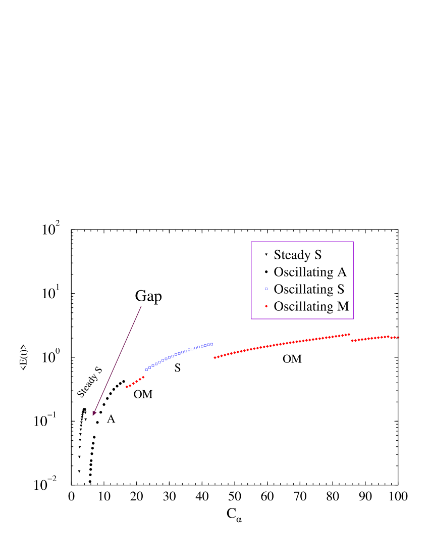
Figure 11: Partial bifurcation diagram, as Fig. 4, for the case of a large polar cut angle, $\theta_{0}=75^{\circ}$, with the generalized Keplerian rotation law, $C_{\omega}=+2.7\times 10^{4}$ ($\partial\Omega/\partial r<0$), $\varpi_{0}=0.3$.

When the sign of the generalized Keplerian rotational shear is reversed (Fig. 12), a steady $A$ mode is again first excited, similar to the case of linear shear. Only for $r_{0}=0.7$ is the behaviour slightly different in that there is a $S$ mode that appears for $C_{\alpha}\approx 22$.

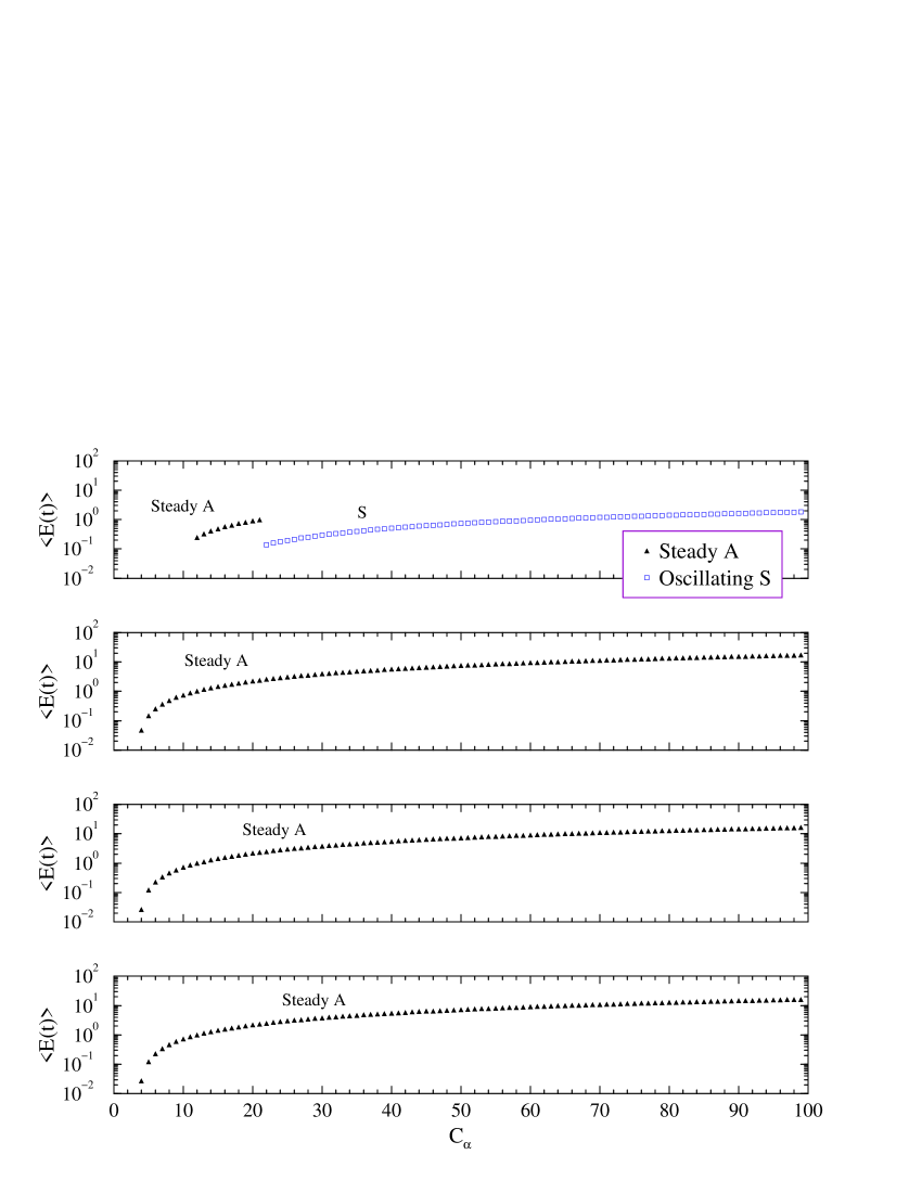
Figure 12: Partial bifurcation diagram, as Fig. 4, for the case of a large polar cut angle, $\theta_{0}=75^{\circ}$, with negative generalized Keplerian rotation law, $C_{\omega}=-10^{4}$ ($\partial\Omega/\partial r>0$), $\varpi_{0}=0.3$.

In the above figures, the nature of the solutions (and thus the symbols shown) are all determined only to within the numerical resolutions chosen and for the length of of time during which solutions were followed and thus in which transients could decay. In particular, near the bifurcation points (as in the case of transitions from pure parity A to S (or vice versa)), we find as expected extremely long transients (at times of more than hundreds of diffusion times). Bearing all this in mind, we do find some evidence which suggests that the conjecture by Jennings & Weiss (1991), according to which transitions from one pure parity to the opposite are mediated by a mixed parity regime, may not always hold. An example of this type of transition is given in Fig. 13, where we have used an exceptionally fine resolution in $C_{\alpha}$. In this case we found after some hundreds of diffusion times that with $C_{\alpha}=4.2868$ and $C_{\alpha}=4.2869$ the parity became $P=+0.9999633$ and $P=-0.9999967$ respectively. A conclusive resolution of this question requires a more substantial study, and we intend to return to this point in a future publication.

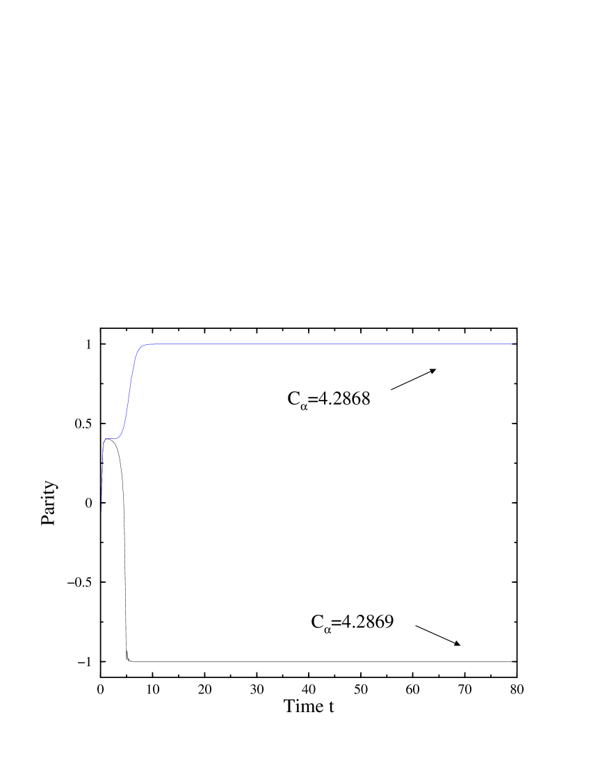
Figure 13: Parity versus time diagram for two runs with same initial conditions except the value of $C_{\alpha}$. The other parameters used were $C_{\omega}=-10^{4}$, $r_{0}=0.2$, $\theta_{0}=45^{\circ}$, with a constant shear rotation profile.

Our results also indicate that overall the behaviour appears to be more complicated in shells than in the full sphere dynamo models, a feature also observed in Covas et al. 1998a.

Also, the nonlinear solutions in configurations which correspond most closely to a thick torus, i.e. $\theta_{0}=22.5^{\circ}$, $r_{0}$ = 0.2, 0.5 and also $\theta=45^{\circ}$, $r_{0}=0.5$, display chaotic behaviour at the lowest values of $C_{\alpha}$. This corresponds with the findings of Brooke & Moss (1994, 1995), that chaotic behaviour was excited at modestly supercritical dynamo numbers in tori, whereas chaotic behaviour only occurred at highly supercritical dynamo numbers in disc and shell configurations.

To obtain an overview of the behaviour of the two parameter family of models considered here, we recall that Table 1 suggests the presence of three different regions with distinct onset behaviours in the parameter space $(r_{0},\theta_{0})$. In the constant shear rotation law case two of these regions possess oscillatory dipolar and quadrupolar onset symmetries respectively and in the third the most readily excited field is steady and quadrupolar. These regions could also be interpreted from a different point of view by considering the behaviour observed in previous dynamo models. Viewed in this way, there are at least two transitions in the $(r_{0},\theta_{0})$ parameter space. The first corresponds to a transition from a region which is consistent with Roberts’ (1972) results (characterised by an $A$ onset mode for $r_{0}<0.7$ and by an $S$ onset mode with $r_{0}\geq 0.7$) to one that does not (i.e. one with antisymmetric onset modes for all $r_{0}$). The second transition is from a disc–like regime in which steady modes are commonly found to one in which they are absent. In order to elucidate this second transition we have made two studies of the parameter space at a finer resolution, by fixing $r_{0}$ and varying $\theta_{0}$ and vice versa. These results are depicted in Figs. 14 and 15 respectively at fixed values of $C_{\alpha}$. (We note that changing the value of $C_{\alpha}$ does not qualitatively change our conclusions.) Those results indicate the presence of two sharp transitions in mean energy and/or parity at around $\theta_{0}\sim 70^{\circ}$ for $r_{0}\sim 0.5$ and $\theta_{0}\sim 75^{\circ}$ for $r_{0}\sim 0.6$. These features are also corroborated by the time series of energy and parity.

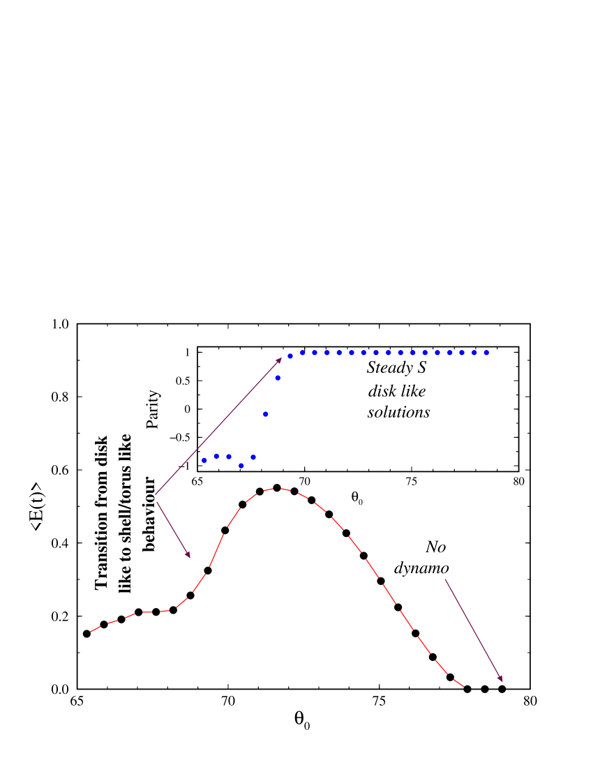
Figure 14: Transition from sphere/shell to disc-like behaviour for a constant shear profile as a function of $\theta_{0}$ for $C_{\alpha}=10$, $r_{0}=0.5$, $C_{\omega}=-10^{4}$. The inset gives the corresponding behaviour of the parity.

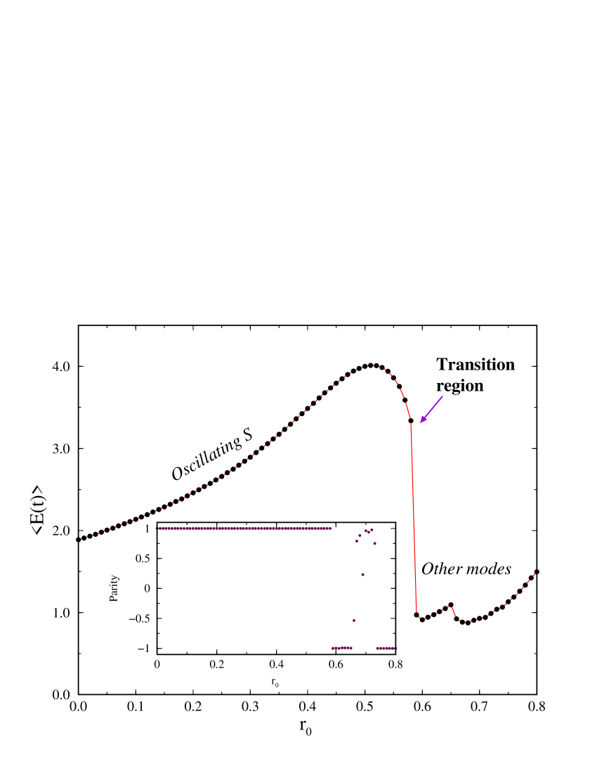
Figure 15: Transition from disc-like to planar like behaviour for a constant shear profile as a function of $r_{0}$ for $C_{\alpha}=60$, $\theta_{0}=75^{\circ}$, $C_{\omega}=-10^{4}$. The inset gives the corresponding behaviour of the parity.

Finally, we have also examined the behaviour of our solutions as a function of the aspect ratio, which we defined as

$$A=\frac{2(1-r_{0})}{(1+r_{0})(\pi-2\theta_{0})}.$$ (14)

With this definition, the smallest aspect ratio corresponds to the configuration with $r_{0}=0.7$ and $\theta_{0}=0$ ($A=0.11$), and the largest to that with $r_{0}=0$ and $\theta_{0}=75^{\circ}$ ($A=3.82$). We find that at large values of $C_{\alpha}$, for example $C_{\alpha}>30$, the averaged energy $\langle E(t)\rangle$ per unit volume of the dynamo region is largest for the configuration with the smallest aspect ratio, and vice versa. In addition, for these values of $C_{\alpha}$, we find that the average energy per unit volume decreases as $\theta_{0}$ increases (i.e. the cuts get larger) and as $r_{0}$ decreases (i.e. the shells get thicker).

4 Conclusions

We have made a comparative study of the dynamical behaviour of a two parameter family of axisymmetric mean-field dynamo models, ranging from a full sphere to shells to torus- and disc-like configurations, within a unified numerical framework. We have found overall agreement with previous studies of axisymmetric mean-field dynamos for spheres, shells, tori and discs. More precisely we find the following:

1. Our results show that changes in both topology and geometry affect the dynamical properties of our models, although these two factors are inevitably interlinked. Specifically, we have three topologically distinct configurations, sphere-like, shell-like and torus-like. Each of these topological configurations can undergo a continuous sequence of geometric changes, from flat objects where the vertical extent is much less than the horizontal, to objects where the vertical and horizontal extents are similar. Our principal findings are that torus-like topologies seem to produce more complex behaviour and that, within a given topological configuration, modest changes in geometry can give rise to different bifurcation sequences. These findings may have considerable astrophysical significance, in that the actual shapes of galaxies and accretion discs often do not conform to the simple geometric shapes used in many studies of mean-field dynamos. Also, since our study concerns the geometry and topology of the dynamo-active region, restrictions of the dynamo-active region in stellar convection zones may have important consequences for the behaviour of the dynamo and these should be taken into consideration when comparing the predictions of dynamo models with observed magnetic behaviour in astrophysical objects.

2. We confirm that the full sphere and shell results of Roberts (1972), concerning the symmetry of the onset modes, are robust with respect to changes in the outer boundary condition, and we extend them to the configurations with very small to medium polar cut angles. Steady modes are found for the largest polar cut angles, agreeing with results from oblate spheroidal geometry. These modes are robust under a change in the rotation law, as found by Walker & Barenghi (1994), except in the case where the configuration resembles a thin torus rather than a disc. In this case an oscillating dipolar solution occurs at onset for a constant shear rotation law, but a steady quadrupolar solution is found with a generalized Keplerian law. In the latter case the steady solution disappears at higher values of $C_{\alpha}$ and there is a gap before an oscillating antisymmetric solution appears. Such a gap was previously observed with a generalized Keplerian rotational profile in both disc (Torkelsson & Brandenburg 1994b) and torus geometry (Brooke & Moss 1995). Stepinski & Levy (1991) also found a similar gap in linear theory. It should be noted that the presence of a gap does depend on the nature of the nonlinearity: it is absent if magnetic buoyancy is the dominant nonlinearity (Torkelsson & Brandenburg 1994a). Our results here indicate the steady solution is also fragile with respect to changes in the rotation law.

3. For the largest polar cut angle, we find evidence for a different mode of behaviour in the thinnest shell ($r_{0}=0.7$) from that found in the thicker shells and full sphere, namely a more complicated behaviour with denser bifurcation sequences, including chaotic and intermittent solutions. Apart from the thinnest shells ($r_{0}=0.7$) the dynamics is qualitatively the same for each sign of the shear. This is consistent with the observation that the thinnest shell approximates a setting in which curvature plays a smaller role.

4. We note a consistent finding in our results, that dynamo-active regions corresponding topologically and geometrically to a torus exhibit chaotic behaviour at lower dynamo numbers compared to spherical, shell-like or disc-like configurations. This concurs with the results of Brooke & Moss (1994,1995), who found transition to chaotic behaviour for a dynamo in a toroidal volume at dynamo numbers that were approximately three times supercritical. Given that the solar (and possibly some stellar) magnetic cycle exhibits irregularity on a variety of time scales, and that many authors have speculated that such behaviour is a manifestation of deterministic chaos, this result may have some astrophysical significance. It therefore seems worthwhile to investigate such dynamos, with a variety of rotational profiles, possibly corresponding to different types of stars, and using different forms of nonlinearity to saturate the field. Since it is the restriction of the dynamo active volume to a toroidal configuration that appears to be important, these dynamos could be considered as embedded in convective shells representing the outer regions of stars.

- (1) Brandenburg, A., 1999, in: Theory of Black Hole Accretion Discs, eds. M. A. Abramowicz, G. Björnsson & J. E. Pringle, Cambridge University Press
- (2) Brandenburg, A., Krause, F., Meinel, R., Moss, D. & Tuominen, I., 1989a, A&A 213, 411
- (3) Brandenburg, A., Moss, D. & Tuominen, I., 1989b, Geophys. Astrophys. Fluid Dyn. 40, 129
- (4) Brandenburg, A., Nordlund, Å., Stein, R. F., Torkelsson, U., 1995, ApJ 446, 741
- (5) Brandenburg, A., Jennings, R. L., Nordlund, Å., Rieutord, M., Stein, R. F., Tuominen, I., 1996, JFM 306, 325
- (6) Brooke J. M. & Moss D., 1994, MNRAS 266, 733
- (7) Brooke, J. M. & Moss, D., 1995, A&A 303, 307
- (8) Covas, E., Tavakol, R., Tworkowski, A. & Brandenburg, A., 1998a, A&A 329, 350
- (9) Covas, E., Tavakol, R., Ashwin, P., Tworkowski, A. & Brooke, J. M., 1998b, submitted to PRL
- (10) Gilman, P.A. & Miller, J., 1981, ApJ Suppl. 46, 211
- (11) Hawley, J.F., Gammie, C.F., & Balbus, S.A., 1996, ApJ 464, 690
- (12) Jennings, R.L., 1991, Geophys. Astrophys. Fluid Dyn. 57, 147
- (13) Jennings, R.L., Weiss, N.O., 1991, MNRAS 252, 249
- (14) Jennings, R.L., Brandenburg, A., Moss, D. & Tuominen, I., 1990, A&A 230, 463
- (15) Jones, C.A., Weiss, N.O., Cattaneo, F., 1985, Physica 14D, 161
- (16) Kitchatinov, L.L., 1987, Geophys. Astrophys. Fluid Dyn. 38, 273
- (17) Krause, F. & Rädler, K.-H., 1980, Mean-Field Magnetohydrodynamics and Dynamo Theory, Pergamon Press, Oxford
- (18) Nordlund, Å., Brandenburg, A., Jennings, R. L., Rieutord, M., Ruokolainen, J., Stein, R.F., Tuominen, I., 1992, ApJ 392, 647
- (19) Rädler, K.-H. 1986, Plasma Physics, ESA SP-251, 569
- (20) Roberts, P. H., 1972, Phil. Trans. Roy. Soc. A272, 663
- (21) Roberts, P.H., Stix, M., 1972, A&A 18, 453
- (22) Ruzmaikin A. A., Sokoloff D. D., Turchaninov V., 1980, Sov. Astron. 24, 182
- (23) Soward, A., 1992a, Geophys. Astrophys. Fluid Dyn., 64, 163
- (24) Soward, A., 1992b, Geophys. Astrophys. Fluid Dyn., 64, 201
- (25) Steenbeck, M., Krause, F., 1969, Astron. Nachr. 291, 49
- (26) Stepinski T.F., Levy E.H., 1991, ApJ 379, 343
- (27) Stix, M., 1975, A&A 42, 85
- (28) Tavakol, R.K., Tworkowski, A.S., Brandenburg, A., Moss, D. & Tuominen, I., 1995, A&A 296, 269
- (29) Tobias, S.M., Weiss, N.O., Kirk, V., 1995, MNRAS 273, 1150
- (30) Torkelsson, U. & Brandenburg, A., 1994a, A&A 283, 677
- (31) Torkelsson, U. & Brandenburg, A., 1994b, A&A 292, 341
- (32) Torkelsson, U. & Brandenburg, A., 1995, Chaos, Solitons & Fractals 5, 1975
- (33) Tworkowski, A., Tavakol, R., Brandenburg, A., Brooke, J. M., Moss, D. & Tuominen, I., 1998, MNRAS 296, 287.
- (34) Walker, M.R., Barenghi, C.F., 1994, Geophys. Astrophys. Fluid Dyn., 76, 265
- (35) Weiss, N.O., Cattaneo, F., Jones, C.A., 1984, Geophys. Astrophys. Fluid Dyn. 30, 305
- (36) Zeldovich, Ya.B., Ruzmaikin, A.A. & Sokoloff, D.D., 1983: Magnetic Fields in Astrophysics, Gordon and Breach, New York.