Selection Effects at 21cm

Abstract

Surveys in the 21cm line of neutral hydrogen are testing the completeness of the catalogs of nearby galaxies. The remarkable observational fact is that the potential wells that confine gas to sufficient density that it can remain neutral in the face of ionizing radiation also provide sites for star formation, so that there are no known cases of neutral intergalactic clouds without associated star light.

Kapteyn Astronomical Institute, P.O. Box 800, 9700 AV Groningen, The Netherlands

1. Introduction

Invisible hydrogen clouds are common place in the vicinity of galaxies. This “low surface brightness” material lies in tidal debris from galaxy interactions (cf. Haynes et al 1979, van der Hulst 1979, Yun et al 1994, Putnam et al 1998), in the extended HI disks that facilitate kinematical studies (cf Broeils & van Woerden 1994), in outlying gas rings around galaxies and pairs of galaxies (Schneider 1989, van Driel et al 1988), in the high velocity clouds around the Milky Way (Wakker and van Woerden 1998), and in a number of other structures for which the nature of the extended LSB gas is less clear (cf. Fisher & Tully 1976, Simkin et al 1987, Giovanelli & Haynes 1989).

Despite vigorous searching, no examples of isolated neutral hydrogen clouds of a truly intergalactic nature have been discovered, and, in fact, for some years, the upper limit to the baryon content of intergalactic clouds with HI masses in the range comparable to normal galaxies has been known to be cosmologically insignificant (Fisher & Tully 1981). This finding is in sharp contrast to the recognition that the ionized intergalactic medium may form an important, perhaps dominant, reservoir of the Universe’s baryons (Rauch et al 1997, Shull et al 1996).

What selection effects influence and limit the neutral hydrogen picture of the nearby universe? What properties could neutral gaseous systems have that would allow them to escape detection in the surveys that have been made so far?

2. Selection Effect ‘0’: the need for neutrals

Clearly, a easy way to hide hydrogen from observers at 21cm wavelength is to ionize it. However, even ionized clouds will have some neutral fraction, and in principle, long integrations with sensitive receivers could detect the 21cm emission from predominantly ionized clouds. The optical depth in the 21cm line of a cloud with neutral $H^{o}$ column density $N_{HI}$, velocity width $\Delta V$ (FWMH) and excitation temperature $T_{spin}$ is

$$\tau_{21}\approx\left(\frac{N_{HI}}{2{\times}10^{21}\;{\rm cm}^{-2}}\right)\left(\frac{10\;{\rm km\;s}^{-1}}{\Delta V}\right)\left(\frac{100\;{\rm K}}{T_{spin}}\right)$$ (1)

Under the conditions for which emission is normally observed from HI clouds (i.e., the excitation temperature is significantly above the temperature provided by the background radiation flux ($T_{spin}\gg 2.7\;{\rm K}$) and $\tau_{21}\ll 1$), the brightness temperature of the emergent radiation from a cloud of neutral $H^{o}$ column density $N_{HI}$ is

$$T_{B}\approx\tau_{21}T_{spin}\approx\left(\frac{N_{HI}}{2{\times}10^{19}\;{\rm cm}^{-2}}\right)\left(\frac{10\;{\rm km\;s}^{-1}}{\Delta V}\right)\;{\rm K}$$ (2)

Under these conditions, the integration time required for a radio telescope to detect a cloud (with $\Delta V\approx 20\;{\rm km\;s}^{-1}$) that fills the telescope beam is approximately one second for $N_{HI}=2{\times}10^{19}$, two minutes for $N_{HI}=2{\times}10^{18}$, and three hours for $N_{HI}=2{\times}10^{17}\;{\rm cm}^{-2}$. The latter column density is of interest because clouds with $N_{HI}\leq 3{\times}10^{17}\;{\rm cm}^{-2}$ are optically thin for wavelengths shortward of the Lyman limit ($\tau_{LL}\leq 1$) and are therefore vulnerable to ionizing radiation with the expectation that the hydrogen within them will be predominantly ionized. For example, it has long been expected that photoionization will cause the outer edges of gaseous galaxy disks to show abrupt declines in the column density of neutral atoms (Sunyaev 1969, Maloney 1993, Corbelli & Salpeter 1993); deep integrations in the outskirts of galaxies and in the intergalactic medium at large, may detect local analogs of the highest column density clouds in the Lyman-$\alpha$ forest and Lyman-limit population identified through quasar absorption-line studies (cf. Hoffman et al 1993, Charlton et al 1994).

Even neutral gas can be hidden from 21 cm emission-line surveys if the excitation temperature $T_{spin}$ is low, as might occur if the gas density is so low that $T_{spin}$ is not coupled to the gas kinetic temperature $T_{k}$ or if $T_{k}$ is intrinsically low. As indicated by Eq. 1, such low $T_{spin}$ clouds would be good absorbers, which should appear in absorption against background continuum sources (cf. Corbelli & Schneider 1990). Of course, in instances when the 21 cm line is optically thick, application of Eq. 2 will underestimate the column density and the HI cloud masses (cf. Dickey et al 1994, Braun 1995, Braun 1997).

3. Selection effect 1: ‘optical selection’ of targets

An historically important selection effect is that the vast majority of extragalactic 21cm line observations have been made with telescopes pointed directly at optically selected objects. Only within the past decade has it become technically feasible to make “optically blind” surveys of sufficiently large volumes of space with adequate sensitivity to recover the known galaxy population, let alone identify new populations of intergalactic clouds or gas-rich LSB galaxies. However, if there were such populations containing HI masses comparable to those in ordinary galaxies and comparable in spatial number density, then the historically important attempts (Shostok 1977, Materne et al 1979, Lo & Sargent 1979, Haynes & Roberts) would have discovered them. The lack of detections in these surveys, combined with the absence of serendipitous detections in the studies targeted on optically selected galaxies, led Fisher and Tully (1981) to conclude that the mass in intergalactic HI clouds in the range $10^{7}$ to $10^{10}M_{\odot}$ could only be a small fraction of the total mass in galaxies, and thus can only contribute a tiny fraction of the total cosmological mass density. Briggs (1990) performed an update of this sort of analysis to conclude that the amount of the HI mass contained in un-identified new populations is only a few percent of HI mass contained in catalogued galaxies over this same mass range.

There have been a few surprises during this period of extensive observation of optically selected targets, including discoveries of uncatalogued HI-rich clouds of undetectably low optical surface brightness (cf. Fisher & Tully 1976, Schneider 1989, Giovanelli & Haynes 1989). However, in every case, the neutral gas is clearly associated in position and redshift velocity with optically visible galaxies, implying that the gravitational potential belonging to the optical galaxy is responsible for the confinement of the hydrogen to sufficient density that it remains neutral.

Similar conclusions result from the recent blind surveys that have been successful at compiling samples of HI-selected galaxies and recovering the known late-type galaxy population (cf. Szomoru et al 1994, Henning 1995, Zwaan et al 1997, Spitzak & Schneider 1998, Kraan-Korteweg et al 1998). All the confirmed HI detections from these surveys are found to be associated with optical emission from star light, provided that the objects are located at sufficiently high galactic latitude that they are not heavily obscured and are not located close to a bright foreground star. This finding lends credence to the idea that a reasonably complete picture of the neutral gas content of the nearby universe can be obtained from a study of the HI gas in the large optically galaxy samples (cf. Rao & Briggs 1993, Briggs 1997).

4. Selection effects for spectroscopic features

Surveys that require the detection of spectroscopic emission features differ in several respects from flux- or magnitude-limited surveys. These differences are illustrated in Fig. 1 and discussed in the following paragraphs.

Until recently, the limitations to radio spectrometer bandwidth and the number of available spectral channels within the spectrometer have often caused surveys to be limited in redshift depth, since they were unable to cover large redshift ranges efficiently. Most of these surveys have sufficient sensitivity to detect large HI masses of $M_{HI}>10^{10}$M_⊙ beyond this restricted survey depth. At the low mass extreme $M_{HI}<10^{7}$M_⊙ nearly all surveys are limited in depth by sensitivity, since integration times become very long to detect these tiny masses at distances of order 10 Mpc or more.

Figure 1.: 21cm Line Detection Sensitivity. Right: The volume probed by a radio telescope beam depends on the beam solid angle $\Omega_{b}$ and the depth $d_{c}$ to which a given HI mass can be detected. For large masses, the detection volume is often limited by the spectrometer bandwidth. Left top: In the “sensitivity limited regime” applicable for small HI masses, the survey volume also depends on velocity width $\Delta V$ shown here for $\Delta V=$ 30, 100 and 300 km s^-1. Left middle: The quantity $({\rm survey\;volume})^{-1}$ specifies a sensitivity function to objects whose space density is $\Phi(M_{HI})$, here given as number per volume per decade of mass. In the low-mass (sensitivity-limited) regime, including the trend of increasing rotation speed with mass implies a sensitivity function $\propto M_{HI}^{-5/4}$ rather than the $M_{HI}^{-3/2}$ dependence for a purely “flux limited” survey. Left bottom: Number of detections expected in bins of 0.2 Dex.

The velocity width of spectral features also influences the detection efficiencies. If two galaxies with the same HI mass $M_{HI}$ are compared, the one with the narrower profile will be easier to detect; the narrower profile could be detected to greater distance. If all galaxies had the same velocity spread, then the limiting distance to which each galaxy could be detected $d_{c}$ would be $\propto M_{HI}^{1/2}$, according to the inverse square law, and the volume within which each could be detected would be proportional to $M_{HI}^{3/2}$. The noise level in flux density, $\sigma$, in a spectrum that has been optimally smoothed to match the profile is $\sigma=\sigma_{o}\sqrt{\Delta v_{o}/\Delta V}$ for a spectrum originally recorded with channel spacing (resolution) of $\Delta v_{o}$ for which the noise level is $\sigma_{o}$. The HI mass for a spectral feature of strength $S_{Jy}$ is computed from the integral over the profile, $M_{HI}=2\times 10^{5}d_{Mpc}^{2}\int S_{Jy}dV_{km/s}M_{\odot}$. Thus, the minimum detectable HI mass is $M_{HI}\propto 5\sigma\Delta Vd^{2}\propto d^{2}\sqrt{\Delta V}$, if the minimum detectable profile is modeled as a rectangle of height in flux density $\Delta S=5\sigma$ and width $\Delta V$. A sort of HI Tully-Fisher relation (cf. Briggs & Rao 1993) has $\Delta V\propto M_{HI}^{1/3}\sin i$ for galaxies with inclination $i$ relative to the plane of the sky, leading to the result that $d_{c}\propto M_{HI}^{5/12}\sin^{-1/4}i$. Note that the $\sin^{-1/4}i$ factor is substantially different from unity for a only small fraction of a randomly oriented sample. The net result is that the survey volume in which a HI mass would be detected is more closely $volume\propto M_{HI}^{5/4}$ in the sensitivity-limited regime. Fig. 1 illustrates the difference in survey volumes for profiles of width 30, 100 and 300 km s^-1. These volumes are translated into survey “sensitivity functions” ($\propto 1/volume$) in units of Mpc^-3 for comparison with HI mass functions; if a survey finds no masses of $10^{7}M_{\odot}$ in a volume of 1 Mpc³, then an estimate of the upper limit to the density of $10^{7}M_{\odot}$ objects is $\sim$1 Mpc^-3.

Figure 1 (left middle panel) illustrates a typical survey mass sensitivity in comparison to an HI mass function $\Phi(M_{HI})$ plotted as number of objects per Mpc^-3 per decade of mass. For mass ranges where the survey sensitivity function lies below the mass function, it become probable that the survey will detect galaxies of that mass. The shaded area represents the mass range where detections should occur in the number as indicated in the lower plot, where detections are binned in 0.2 decade bins. In the regions below ${\sim}10^{7.3}$ and above ${\sim}10^{10.1}$, this survey would probably obtain no detections but could place upper limits on the space density of galaxies in these mass ranges.

The knowledge of the space density of tiny HI-rich extragalactic objects has remained highly uncertain because of the difficulty in surveying a sufficiently large volume with adequate sensitivity to detect them. A further complication is that the small masses have narrow velocity widths without the distinctive double horned profiles that characterize large spiral galaxies with flat rotation curves; this means that low mass systems can be more easily confused with radio interference.

The poor diffraction-limited angular resolution provided by most single-dish radio telescopes gives rise to confusion problems, and many detections in blind surveys may be multiple galaxy systems. Small galaxies in close proximity to large ones can easily be missed, if their redshift velocities fall within the range spanned by the emission profiles of bright, dominant galaxies.

4.1. Computation of the HI-mass function

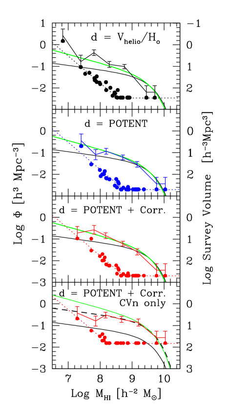
Figure 2.: HI-mass function for the Canis Venatici survey volume (Kraan-Korteweg et al 1998), normalized to number of objects per decade of mass. The smooth solid curve is the analytic form derived by Zwaan et al (1997) with a slope of $\alpha=-1.2$, the grey line has a slope of $\alpha=-1.4$ (Banks et al 1998). The bottom panel shows the result restricted to the CVn-group regions ($<$1200 km s^-1), and the dashed curve represents the Zwaan et al HI-mass function multiplied by a factor of 4.5. The dotted line in each panel gives an indication of the volume probed as a function of mass (see right vertical axis); the points give 1/V_max for each of the galaxies in the sample, taking into account the different velocity widths.

A number of subtle effects enter when the space density of gas-rich galaxies, the HI-mass function, is constructed. These problems are especially acute for the small HI masses, which can only be detected in blind surveys if the objects are very close by. Some of these problems, including the effects of peculiar velocities, deviations from pure Hubble flow, and large-scale fluctuations in density, are illustrated in Fig. 2, which presents the recent Nançay optically-blind, 21cm line survey of the Canis Venatici region. First, the top panel shows the number density of galaxies as computed using distances, HI masses, and sensitivity volumes based on conversion of heliocentric velocities to distance $V_{hel}/H_{o}$. The mass functions are binned into half-decade bins, but are scaled to give number of objects per decade. The value for each decade is computed from the sum $\Sigma\;1/V_{max}$, where V_max is the volume of the survey in which a galaxy with the properties $M_{HI}$ and $\Delta V$ could have been detected. A steeply rising, low mass tail results from this calculation due to one galaxy, UGC 7131, which is is treated in this naive calculation as a very nearby, but low mass object. Placed at the greater distance implied by independent distance measurement (Makarova et al 1998), it becomes more massive, and it finds its place among other galaxies of greater velocity width and higher HI mass in the higher mass bins, as shown in the lower panels.

An improved calculation based on POTENT distances, which include local deviations from uniform Hubble expansion (Bertschinger et al 1990), is displayed in the second panel. In the third panel, four galaxies from the Nançay sample with independent distance measurements have been plotted according to their revised distances. In the 4th panel we have restricted our sample to include only the overdense foreground region that contains the CVn and Coma groups, i.e. the volume within $V_{hel}<$1200 km s^-1 and about 1/2 the RA coverage (about half the solid angle) of the full survey. Large HI-mass galaxies can be detected throughout the volume we surveyed, but small galaxies can be detected only in the front part of our volume. The volume normalization factors, which are used to compute the mass function, are sensitivity limited for the small masses to only the front part of our survey volume. For the large masses, the V_max’s include the whole volume, including the volume where the numbers of galaxies are much less. Hence, when restricting the “survey volume” we get a fairer comparison of the number of little galaxies to the number of big ones.

In all four panels the solid line represents the HI-mass function with a slope of $\alpha=-1.2$ as derived by Zwaan et al (1997), whereas the grey line represents an HI-mass function with a slope of $\alpha=-1.4$ as deduced by Banks et al (1998) for a survey in the CenA-group region. Restricting our volume to the dense foreground region including “only” the CVn and Coma groups, we find that the Zwaan et al HI-mass function with a scaling factor of 4.5 to account for the local overdensity (dashed line in the bottom panel) gives an excellent fit to the data.

Clearly the computation of mass functions for tiny dwarfs will remain vulnerable to subtleties, due to the small volumes in which they can be detected and the accompanying uncertainties in distance.

5. Conclusion: physical selection

The largest reservoirs of HI gas in the nearby universe are found in large galaxies. The bulk of the HI associated with low optical surface brightness falls in the outskirts of large galaxies. Apparently an additional consequence of the gravitational confinement that preserves gas neutrality is the production of stars, since no cases of free-floating HI clouds away from galaxies have been found. Deep integrations in the 21cm line over long sightlines should eventually detect the highest column density clouds of the ionized Lyman-$\alpha$ forest.

References

Banks, G.D., Disney, M.J., Knezek, P., et al 1998, in prep

Bertschinger, E. et al 1990, ApJ, 364, 370

Braun, R. 1997, ApJ, 484, 637

Braun, R. 1995, BAAS, 187, 6501

Briggs, F.H., & Rao, S. 1993, ApJ, 417, 494

Briggs, F.H. 1997, ApJ, 484, 618

Broeils, A.H., van Woerden, H. 1994, A&AS, 107, 129

Charlton, J.C., Salpeter, E.E., & Linder, S.M. 1994, ApJ, 430, L29

Corbelli, E., & Salpeter, E.E. 1993, ApJ, 419, 104

Corbelli, E., & Schneider, S.S. 1990, ApJ, 356, 14

Dickey, J.M., Mebold, U., Marx, M., et al 1994, A&A, 289, 357

Fisher, J.R., & Tully, R.B. 1976, A&A, 53, 397

Fisher, J.R., & Tully, R.B. 1981, ApJ, 243, L23

Giovanelli, R. & Haynes, M.P. 1989, ApJ, 346, L5

Haynes, M.P., & Roberts, M.S. 1979, ApJ, 227, 767

Haynes, M.P., Giovanelli, R., & Roberts, M.S. 1979, ApJ, 229, 83

Henning, P.A. 1995, ApJ, 450, 578

Hoffman, G.L., Lu, N.Y., Salpeter, E.E., et al 1993, AJ, 106,39

Kraan-Korteweg, R.C., van Driel, W., Briggs, F.H., Binggeli, B., & Mostefaoui, T.I. 1998, A&A, in press

Lo, K.Y., & Sargent, W.L.W. 1979, ApJ, 227, 756

Maloney, P. 1993, ApJ, 414, 41

Materne, J., Huchtmeier, W.K., & Hulsbosch, A.N.M. 1979, MNRAS, 18, 563

Putnam, M.E. Gibson, B.K., Staveley-Smith, L., et al 1998, Nature, 394, 742

Rao, S.M., & Briggs, F.H. 1993, ApJ, 419, 515

Rauch, M., et al 1997, ApJ, 489, 7

Schneider, S.E. 1989 , ApJ, 343, 94

Shostok, G.S. 1977, A&A, 54, 919

Shull, J.M., Stocke, J.T., & Penton, S. 1996, AJ, 111, 72

Simkin, S.M., Su, H-J., van Gorkom, J., Hibbard, J. 1987, Sci, 235, 1367

Spitzak, J., & Schneider, S.E. 1998, ApJS, in press

Sunyaev, R.A. 1969, Astrophys.Lett., 3, 33

Szomoru, A., Guhathakurta, P., van Gorkom, J.H., Knapen, J.H., Weinberg, D.H., & Fruchter, A.S. 1994, AJ, 108, 491

van der Hulst, J.M. 1979, A&A, 75, 97

van Driel, W., van Woerden, H., Schwarz, U.J., & Gallagher, J.S. 1988, A&A, 191, 201

Wakker, B.P., & van Woerden, H., 1997, ARA&A, 35, 217

Yun, M.S., Ho, P.T.P., & Lo, K.Y. 1994, Nature, 372, 530

Zwaan, M.A., Briggs, F.H., Sprayberry, D., & Sorar, E. 1997, ApJ, 490, 173