QSO Absorption Line Systems

It is difficult to describe in a few pages the numerous specific techniques used to study absorption lines seen in QSO spectra and to review even rapidly the field of research based on their observation and analysis. What follows is therefore a pale introduction to the invaluable contribution of these studies to our knowledge of the gaseous component of the Universe and its cosmological evolution. A rich bibliography is given which, although not complete, will be hopefully useful for further investigations. Emphasis will be laid on the impact of this field on the question of the formation and evolution of galaxies.

1 INTRODUCTION

Although steady progress is made towards detecting faint objects in emission, the high-redshift objects detected this way up to now are drawn from a particular population of powerful emitters (e.g. [88]). On the contrary, absorption may reveal standard objects such as a normal galaxy or intergalactic gaseous clouds close enough to the line of sight to QSOs all over the range of accessible redshifts from zero to the highest QSO redshift $z$ = 4.897 [78]. A typical spectrum is shown in Fig. LABEL:Fig1. Absorption line systems observed in QSO spectra are generally classified into three categories:

(1) The metal-line systems in which a large number of elements, in different ionization stages, is observed, from C i to C iv or O i to O vi. The Lyman limit systems (LLS) are optically thick at the H i Lyman limit (912 Å) and have therefore H i column densities $N$(H i) $>$ 2$\times$10¹⁷ cm^-2. They are closely related, at any redshift, to galaxies. The latter have been detected by direct imaging and follow-up spectroscopy at low and intermediate redshift[4, 30, 86]. Studying their number density and physical properties (kinematics, ionization state, abundances) is then a unique tool to trace galaxy formation. Among these systems, the rare damped systems, characterized by a very large H i column density ($N$(H i) $>$ 2$\times$10²⁰ cm^-2) are often considered to be associated with galactic disks or protogalactic disks[98].

(2) The Ly$\alpha$ lines with no metal lines detected at the same redshift, are of intergalactic origin at high redshift (e.g. [76]) but could somehow be associated with galaxies at low redshift[43]. Information about these systems (column density, Doppler parameter, kinematics, clustering) is derived from line-profile fitting. The latter requires high-resolution high-quality spectra that are difficult to obtain on 4m-class telescopes. Recent studies of absorptions coincident in redshift in the spectra of gravitationally lensed QSO images [79] or QSO pairs (e.g. [22]) have shown that the mean radius of the absorbers is surprizingly large (up to 500 kpc). The idea that the Ly$\alpha$ gas could trace the potential wells of dark matter [10] and reveal its characteristical filamentary structure has been successfully investigated using $N$-body simulations [58, 64].

(3) The broad absorption line (BAL) systems are characterized by impressive absorption troughs from different ions of low and high excitation, extending from 0 up to 60000 km s^-1 outflow velocity relative to the QSO emission redshift. It is widely accepted that the gas is very close to the centre of the QSO host-galaxy and may be part of the broad emission line region ([96, 92], see also [33]). They thus are intimately related to the AGN phenomenon. Although AGN activity is an important factor of galaxy formation, the role of BAL systems in galaxy formation is unclear at the moment. This is the bad reason why they are not described in this lecture.

2 ABSORPTION LINES

In this Section, we summarize a few basic and classical results on the formation and characteristics of absorption lines, that are important to keep in mind when discussing the scientific issues presented in the following Sections.

2.1 Definitions

An absorption line has an equivalent width $w_{\rm obs}$ in Å  defined as:

$$w_{\rm obs}=\int{I_{\rm c}-I\over I_{\rm c}}d\lambda=\int(1-e^{-\tau(\lambda)})d\lambda$$ (1)

where $I$ is the observed spectral intensity, $I_{\rm c}$ the interpolation of the absorption-free continuum over the absorption feature and $\tau(\lambda)$ the optical depth. It is apparent from Eq.(1) that the observed equivalent width does not depend on the spectral resolution. For redshifted absorption lines, $w_{\rm obs}$ = $w_{\rm rest}$$\times$(1+$z_{\rm abs}$).

If we assume that the absorbing atoms have a gaussian velocity distribution of mean $v_{\rm o}$ relative to the referential $R$, then it is possible to estimate the optical depth in Eq.(1) as seen by an observer in $R$. An atom with velocity $v$ absorbs a photon of frequency $\nu$ in $R$ with a cross-section $\sigma$($\nu^{\prime}$) where $\nu^{\prime}$ = $\nu$/(1-$v/c$), $v$ taken to be positive for an atom that goes away from the observer and,

$$\tau(\nu)=N{1\over{\sqrt{\pi}}b}\int^{+\infty}_{-\infty}\sigma(\nu^{\prime})e^{-{(v-v_{\rm o})^{2}\over b^{2}}}dv$$ (2)

where $N$ is the column density, the total number of atoms per surface unity integrated over the gaussian distribution centered at $v_{\rm o}$ on the line of sight; $b$ is the Doppler parameter, $b$ = $v_{\rm rms}$${\sqrt{2}}$ = $FWHM$/2${\sqrt{Ln2}}$; $FWHM$ is the full width at half maximum. When the velocity field is not turbulent, the Doppler parameter is related to the temperature of the gas by

$$b_{\rm th}={\sqrt{2kT\over m}}=12.8{\rm(km\;s^{-1})}{\sqrt{T_{4}\over M}}$$ (3)

where $m$ is the mass of an atom, $M$ its mass number and $T_{4}$ = T/10⁴ K. In case the turbulence can be modelled as a gaussian velocity distribution with quadratic mean velocity ${\sqrt{3\over 2}}V$ and mean velocity 2$V/{\sqrt{\pi}}$, then $b_{\rm tot}^{2}$ = $b_{\rm th}^{2}$ + $V^{2}$.

The cross-section for the absorption in an atomic transition is characterized by an absolute (classical) value, modulated by the oscillator strength $f$ and a frequency dependence which is a consequence of the finite life-time of the upper level:

$$\sigma=f\times{1\over 4\pi\epsilon_{\rm o}}{\pi e^{2}\over m_{\rm e}c}\times{1\over\pi}{{\gamma\over 4\pi}\over(\nu-\nu_{\rm o})^{2}+({\gamma\over 4\pi})^{2}}$$ (4)

where the usual notations for the fundamental physical constants have been used and $\gamma$ is the total damping constant (de-excitation rate of the upper level). Eq.(2) reduces to

$$\tau(\lambda)=1.498\times 10^{-2}{Nf\lambda\over b}H(a,u)$$ (5)

with

$$H(a,u)={a\over\pi}\int^{+\infty}_{-\infty}{e^{-y^{2}}\over(u-y)^{2}+a^{2}}dy;\;a={\lambda\gamma\over 4\pi b};\;u=-{c\over b}\left((1+{v\over c})-{\lambda\over\lambda_{\rm o}}\right)$$ (6)

$H(a,u)$ is called the Voigt function which is a convolution of a gaussian function and a lorentzian function.

The optical depth at the center of the line is:

$$\tau_{\rm o}=1.497\times 10^{-15}{N{\rm(cm^{-2})}f\lambda_{\rm o}{\rm(\AA)}\over b{\rm(km\;s^{-1})}}$$ (7)

More details can be found in e.g. [56].

2.2 The Voigt Profile

Under the assumption that the velocity distribution of the atoms is described by a Gaussian function, the overall shape of the optical depth $\tau$ over the absorption line is a Voigt function. The core of the Voigt function is gaussian and the far wings are lorentzian. The absorption feature itself, which is simply $e^{-\tau}$, is called a Voigt profile. The different regimes are illustrated on Fig. 2.

The absorption of photons with wavelength $\lambda$1, or on a velocity scale $V_{1}$ = $c(\lambda_{1}-\lambda_{0})/\lambda_{0}$, is due to a continuous sum of contributions by the atoms with different velocities. The probability that atoms 1 of velocity 0 absorb the photons $\lambda_{1}$ is given by the value of the lorentzian at $V_{1}$. Since $V_{1}$ is close to the center of the absorption line, it is apparent that atoms 2 of velocity $V_{1}$ will dominate the absorption because the variations of the lorentzian is much faster than the variations of the gaussian from 0 to $V_{1}$. The variations of the optical depth in the core of the line will thus be governed by the gaussian function. In contrast, the absorption of photons with wavelength $\lambda_{2}$, or on a velocity scale $V_{2}$ = $c(\lambda_{2}-\lambda_{0})/\lambda_{0}$, is dominated by atoms with velocity 0. Indeed, far from the center of the line, the variations of the gaussian function are much faster than the variations of the lorentzian. The number of atoms with velocity $V_{2}$ is negligible. If absorption is seen at $\lambda_{2}$, this is due to the non-negligible probability of an atom 1 to absorb a photon with wavelength $\lambda_{2}$. Of course, the total column density must be large for the optical depth to be non negligible in the wing. Thus when using the sketch of Fig. 2, it must be noticed that the transition between both regimes is very sharp around $u$ $\sim$ $\pm$3.2 (see Eq.6) which corresponds to more than twice the FWHM. This is why the damping wings are prominent only for strong lines.

Fig. 2.—: Illustration of the formation of the Voigt profile: over the profile, the optical depth has a gaussian shape in the core of the absorption line and lorentzian shape in the extended wings (see the text). The functions have arbitrary widths and are normalized to one at the maximum.

Of course the assumption of a gaussian velocity distribution can be questioned. Under other assumptions, the absorption profile can be significantly different from a Voigt profile. This is particularly important when discussing the characteristics of the absorptions derived from line profile fitting (see [41, 47, 48]).

2.3 The Curve of Growth

Fig. 3.—: Curve of growth: logarithm of the equivalent width ($w$ in Å) versus logarithm of the column density ($N$ in cm^-2) for different values of the Doppler parameter ($b$ in km s^-1). The curves are calculated for H i Ly$\alpha$1215. The three characteristic regimes are illustrated (see the text).

From Eqs.(2)(6)(1) one can calculate the curve of growth which is the relation between the equivalent width of a line and the column density for different values of the Doppler parameter. The curve of growth for the H i Ly$\alpha$ transition is plotted on Fig. 3 for $b$ = 5, 10, 20 and 30 km s^-1.

There are three distinct regimes:

$\bullet$ When the column density is small ($\tau_{\rm o}$ $<$ 0.1), the absorption line is optically thin and the equivalent width does not depend on $b$. This is the linear part of the curve of growth, where the determination of $N$ from $w$ is easy and reliable. For any transition,

$$N{\rm(cm^{-2})}=1.13\times 10^{20}{w_{\rm r}{\rm(\AA)}\over\lambda^{2}{\rm(\AA)}f}$$ (8)

Fig. 3 shows that for H i$\lambda$1215, a log $N$ = 13 line is partially saturated whatever the $b$ value is.

$\bullet$ The logarithmic or flat-part of the curve of growth is characterized by the large dependence of $N$ on $b$ at a given $w$. In this regime, the determination of $b$ and $N$ are very uncertain except when several lines of the same ion are used. Equivalent width and optical depth at the center of the line (see Eq.7) are related by:

$${w\over\lambda_{\rm o}}=2{b\over c}{\sqrt{Ln(\tau_{\rm o})}}$$ (9)

$\bullet$ The absorption lines that are on the saturated part of the curve of growth are characterized by prominent damping wings. The equivalent width does not depend on $b$ and the column density determination from measurement of $w$ or fitting the wings is very accurate. In that case (see Eqs.6 and 7),

$${w\over\lambda_{\rm o}}=2.64{b{\sqrt{a}}\over c}\times{\sqrt{\tau}_{\rm o}}$$ (10)

For H i$\lambda$1215, $\gamma$ = 6.265$\times$10⁸ s^-1 [56] and:

$$N{\rm(cm^{-2})}=1.88\times 10^{18}w_{\rm rest}^{2}{\rm(\AA)}$$ (11)

Fig. 3 shows clearly that, for realistic values of $b$, the H i$\lambda$1215 transition is in this regime for log $N$ $>$ 19. The definition of damped systems as absorbers with log $N$(H i) $>$ 20.3 is artificial and was introduced to search for damped candidates in low spectral resolution data (see [97]). Indeed, for such column densities, the absorption line has $w_{\rm obs}$ $>$ 15 Å  at $z$ $>$ 2. The probability that such a feature be the result of blending of weaker lines is small. For smaller column densities, the probability for such confusion is much higher.

The values of $\lambda$ and $f$ are given for illustration for a few transitions in Table 1. A more complete list can be found in [57][94][77].

Note that most of the transitions are from the true ground state. Exceptions are found (i) when the excited levels of the ground-state are populated by pumping from the true ground-state by the background radiation (C i^∗$\lambda\lambda$1560,1656, e.g. [82], this leads to determinations of the CMB temperature at high $z$; C ii^∗$\lambda$1334, e.g. [46], is used to derive limits on the electronic density) and (ii) in a few associated or BAL absorption systems in which the density is high enough for upper levels to be populated by collisional excitation (e.g. [96]).

Table 1. A few strong atomic transitions
Ion	$\lambda_{\rm o}$	f	log($\lambda_{\rm o}$f)	log($\lambda_{\rm o}^{2}$f)
	(Å)
O vi	1031.927	0.130	2.128	5.141
O vi	1037.616	0.0648	1.828	4.844
H i	1215.670	0.4162	2.704	5.789
O i	1302.169	0.0486	1.801	4.916
C ii	1334.532	0.118	2.197	5.323
Si iv	1393.755	0.528	2.867	6.011
Si iv	1402.770	0.262	2.565	5.712
C iv	1548.202	0.194	2.448	5.667
C iv	1550.774	0.097	2.177	5.368
Mg ii	2796.352	0.592	3.219	6.666
Mg ii	2803.531	0.295	2.918	6.365

The column density and Doppler parameter for an ion can be formaly determined if two transitions from the same lower level are observed on the flat part of the curve of growth. Indeed from Eqs.(9) and (7) it is easy to extract $N$ and $b$. This is the doublet method which has been extensively used because doublets are numerous and easily observed (see Table 1). Of course the parameters are better determined when more than two lines from the same level are used.

2.4 Fitting the Lines

In practice however the problem is complicated by the structure of the absorber. Most often, an absorption feature is a blend of several components. Indeed when the line of sight passes for example through a galactic halo, it can intercept several clouds. The relative projected velocities of the clouds are usually not very large (typically $\Delta V$ $<$ 150 km s^-1) compared to the width of the lines (5 to 50 km s^-1 or larger) and the number of clouds can be large (more than ten). Column densities and Doppler parameters for each component are derived from line profile fitting, using the maximum of transitions. This is illustrated on Fig. 4 for H i. The fit of a single absorption feature with several components is most often not unique; the different solutions can yield column densities differing by an order of magnitude. When several transitions from the same ion are used, as the transitions in the Lyman series for H i, better significance is achieved. Stronger constraints can be put on models by using several ions. Indeed metal lines are narrower than H i lines and column densities are usually smaller for metals than for H i, so that metal absorption features are relatively less sensitive to blending effects (see Fig. 5). However it must be assumed that the decomposition in components is the same for the different ions. Hence, it is usually a good assumption to consider that H i, O i, Si ii, C ii, Al ii and Fe ii on the one hand, and C iv and Si iv on the other arise in the same phase and can be fitted together (see Fig. 5).

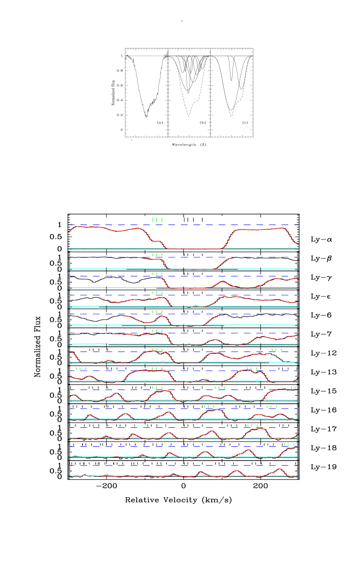
Fig. 4.—: Upper panel: The fit of a single absorption line (here H i$\lambda$1215; from Fernandez-Soto et al. [26]) is by no means unique; to constrain the model, several transitions are used, either from the same ion (in the lower panel all the H i transitions in the Lyman series are used; from Burles & Tytler [8]; note that the model is overplotted to the data) or from different ions assumed to arise in the same phase.

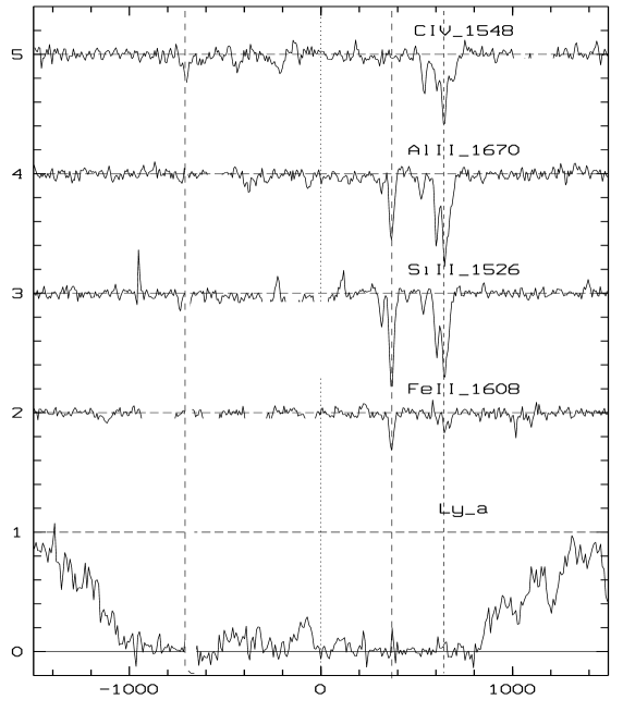
Fig. 5.—: Absorption lines in the $z_{\rm abs}$ = 3.1825 system toward PKS 2000–330 plotted on a relative velocity scale. Parts of the spectrum have been removed when absorption lines from other systems were present. It is apparent that (i) the metal lines are much narrower than the H i line; note however that metallicity in the system is quite low, of the order of 1/100 of solar; (ii) the number of components needed to fit the H i line is much larger than for the metal lines; (iii) the position of three metal components have been marked by dashed vertical lines; it can be seen that the velocity coincidence is very good between Si ii, Al ii and Fe ii.

Several procedures using $\chi^{2}$ minimization techniques are available to perform Voigt profile fitting of the absorption features. The most popular are FITLYMAN implemented in MIDAS the ESO image processing package (Fontana & Ballester [27]) and VPFIT (Carswell et al. [9]). To visualize the lines XVOIGT is also very convenient (Mar [51]). Most of the models overplotted on the figures have been created with the latter procedure.

3 THE LY$\alpha$ FOREST

The numerous H i lines seen in the Ly$\alpha$ forest correspond to the imprint left by the intergalactic medium in the QSO spectrum. The whole redshift interval from zero to the highest QSO emission redshift has been observed. A review of the recent works and ideas on this subject can be found in [73]. In the following, a few important observations and interpretations are highlighted.

3.1 Evolution of the Number Density of Lines

The redshift evolution of the number of Ly$\alpha$ lines per unit redshift is usually fitted by a power law,

$$N(z)=N_{\rm o}(1+z)^{\gamma}$$ (12)

Note that $N_{\rm o}$ depends on the equivalent width; weak lines are more numerous than strong lines (see next Section). The observed exponent $\gamma$ can be compared with that expected if the forest is due to a non-evolving population:

$${\gamma}=2-{1\over 2}[3\Omega_{\rm o}(1+z)^{3}-2K_{\rm o}(1+z)^{2}]\times[\Omega_{\rm o}(1+z)^{3}-K_{\rm o}(1+z)^{2}+{\Lambda\over 3H_{\rm o}^{2}}]^{-1}$$ (13)

with standard notations and with $K_{\rm o}$ = $\Omega_{\rm o}$+${\Lambda\over 3H_{\rm o}^{2}}$–1 (see [28]). For a model without a cosmological constant,

$${\gamma}=(1+q_{\rm o}z-q_{\rm o})(1+2q_{\rm o}z)^{-1}$$ (14)

In the absence of evolution, the exponent is equal to 1.0 for $q_{\rm o}$ = 0 and 0.5 for $q_{\rm o}$ = 0.5 at $z$ = 2. Observations show that the Ly$\alpha$ forest evolves strongly at high redshift ([40]; $\gamma$ $\sim$ 2.5 at $z$ $\sim$ 2); that weak lines evolve more slowly than stronger one; and that there is a break at $z$ $\sim$ 1.5 in the cosmological evolution of the number density of lines (see Fig. 6, [38]).

Fig. 6.—: Logarithm of the number density of Ly$\alpha$ lines versus redshift from Jannuzi et al. [38]. The break at $z$ $\sim$ 1.5 is apparent.

3.2 Column Density Distribution

The column density distribution for all absorption systems (the Ly$\alpha$ forest corresponds only to the smallest column densities) at $z$ $\sim$ 2.8 is shown on Fig. 7. The best fit for the forest is a power-law d${}^{2}n$/d$N$d$z$ $\propto$ $N^{-1.5}$. There is a deficit of lines at $N$ $\sim$ 10¹⁵ cm^-2 and a flatening of the distribution for the damped systems [40, 66]. These features have been interpreted as a consequence of the structure of the intergalactic medium and of different ionization effects [12, 25, 63]. It has been shown from this distribution that the Ly$\alpha$ forest at high redshift contains most of the baryons in the Universe [66], a result that has been confirmed by other methods [70, 52]. This suggests that at high redshift, the intergalactic medium is the reservoir of baryons for galaxy formation.

Fig. 7.—: H i column density distribution at $z$ $\sim$ 2.8 from Hu et al. [35] and Petitjean et al. [66]. There is a deficit of lines at $N$ $\sim$ 10¹⁵ cm^-2.

3.3 Physical Conditions

The density of the gas must be very small. Indeed from coincident absorptions along adjacent lines of sight (see below, e.g. [3, 21]), it can be shown that the gas in the Ly$\alpha$ forest is fairly uniform on scales of $\sim$1 kpc. This implies that for a typical column density of $N$(H i) = 10¹⁴ cm^-2, the H i density is smaller than 3$\times$10^-8 cm^-3. Even for an ionization correction factor corresponding to highly ionized gas, $n$(HII)/$n$(HI) = 10⁴, the total density is smaller than 3$\times$10^-4 cm^-3.

The intergalactic gas is exposed to the effect of the UV-background which is the radiation field produced by QSOs and early galaxies at high redshift. It is possible to estimate the flux at the Lyman limit using the observed number of sources (e.g. [53, 72]), $J_{912}$ $>$ 2.3$\times$10^-22 erg/s/cm²/Hz/sr at $z$ $\sim$ 2.5 if the shape of the ionizing spectrum is taken as in [31]. With the above orders of magnitude the ionization parameter is $U$ = 0.02 and the gas is indeed completely ionized.

The presence of metals in the Ly$\alpha$ forest is an important clue towards understanding how and where the first objects in the universe formed. It has been known for long that the amount of metals is small. However given the small column densities involved, the question could not be satisfactorily answered before the advent of the 10m-class telescopes. Using Keck data, it has been shown recently that C iv absorption is seen in all the systems with log $N$(H i) $>$ 15 and in half of the systems with log $N$(H i) $>$ 14.3 [16, 93, 81]. A lower limit on the metallicity, $Z$ $>$ 10^-3 $Z_{\odot}$ ($H_{\rm o}$ = 65, $q_{\rm o}$ = 0.02), is derived after difficult ionization corrections [80]. The production of this amount of metals would induce enough photons to completely pre-ionized the IGM [55]. However, it is much lower than the predictions of metal production by a first generation of Type II supernovae [55]. The presence of metals in systems with smaller column densities is still controversial [17, 50].

Another way to estimate the ionizing UV-background is to use the proximity effect which is the observed decrease of the number of absorption lines at a given equivalent width limit in the vicinity of the QSO. This is interpreted as a consequence of the enhanced ionizing flux due to the emission by the quasar. The radius of influence of the quasar emission can thus be derived from observations. This is the distance from the QSO at which the depleted number density of lines reaches to the background value. At this point, to a first approximation, the flux from the background is comparable to the flux from the quasar [1]. However this determination assumes that (i) the number density of clouds can be extrapolated toward the quasar (this may be wrong if the density of clouds increases in the potential wells of the QSO), (ii) the luminosity of the QSO is known from direct observation (questionable if variability occurs), (iii) the redshift of the quasar is known (discrepancies between different lines are the rule, [23]). From this it is easy to understand that the typical value of $J_{912}$ $\sim$ 10^-21 erg/s/cm²/Hz/sr derived from these studies is highly uncertain. The uncertainties are discussed in [2, 29] and in more detail in [15].

3.4 Clustering Properties

The two-point correlation function $\xi$ has been studied by several authors with contradictory conclusions, probably because the number of lines of sight was not large enough. Cristiani et al. [18] use 1600 lines and show that there is a strong signal on scales $\Delta v$ $<$ 200 km s^-1 which increases for increasing column densities. However, it is difficult to disentangle the large scale clustering signal from the effects of the internal structure in an absorber [26]. Indeed, the column density through a system increases because the number of subcomponents increases; each component beeing the signature of an individual cloud in an extended halo [62]. This is why observers have tried to measure directly the dimensions of absorbing clouds. For this, they use pairs or groups of quasars with small angular separations on the sky. Correlation of absorption features along the different lines of sight indicates that the characteristic size of the absorbers is larger than the projected separation of the lines of sight. In the spectra of multiple images of lensed quasars with separations of the order of a few arcsec [79, 37], the Ly$\alpha$ forests appear nearly identical, implying that the absorbing objects have large sizes ($>$50 kpc). For larger separations between lines of sight, the correlation between the two forests decreases; however after random coincidences are removed, an excess of common redshift absorption exists even for separations as large as 500 $h^{-1}$ kpc [20]. This suggests very large dimensions or at least that the clouds are closely correlated on these scales. The data available up to now have been critically analyzed by D’Odorico et al. [22] who concluded that the absorbers have typical sizes of the order of $R$ $\sim$ 350$\pm$100$h^{-1}$ kpc. The number of suitable groups of quasars is too small at present to constrain the structure of the Ly$\alpha$ complexes. However, it is easy to see that the method is very powerful to study the correlation of baryonic matter at high redshift. The number of observable pairs should increase dramatically with the advent of 10m-class telescopes. It is also conceivable, although ambitious, to probe the 3D-distribution of the gas in a small field by increasing the density of lines of sight. To this aim, quasars with magnitude 22 should be observed at intermediate resolution. The large amount of telescope time needed requires multi-object spectroscopy capabilities on 10m-class telescopes [60]. If a hundred lines of sight could be observed in one square degree, the probability distribution function of the matter density could be investigated at high redshift. This would be a unique way to study how galaxy formation is related to the distribution and dynamics of the underlying matter field (see [59, 19] and next Section). The method is illustrated in Fig. 8.

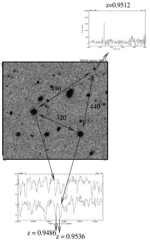
Fig. 8.—: Observation of a quasar pair [65]: Q1026–0025A ($z_{\rm em}$ = 1.438; situated in the bottom right corner of the image) and B ($z_{\rm em}$ = 1.526; 36 arcsec or 320$h^{-1}_{50}$ kpc away from A in the north-east direction). North is at the top, east to the left. Ly$\alpha$ absorptions are seen at $z_{\rm abs}$ = 0.9486 and 0.9536 in the HST spectrum of A and at $z_{\rm abs}$ = 0.9486 in B. A galaxy is detected with the NTT (ESO-La Silla) at redshift $z_{\rm em}$ = 0.9512 at a projected distance of $\sim$ 450 kpc from the two absorbers. Using 10m-class telescopes, it will be possible to observe $m$ $\sim$ 22 magnitude quasar at intermediate resolution. The aim is to increase the density of lines of sight in order to study the 3D spatial distribution of the gas and to correlate this distribution with the galaxies in the field.

3.5 Simulations

Most models of the Ly$\alpha$ forest assume that the intergalactic medium is populated by diffuse clouds, either gravitationally or pressure confined, and possibly embedded in a pervasive medium (e.g. [6, 76, 74, 36]). A more attractive picture arised recently from large-scale dark-matter $N$-body simulations including a description of the baryonic component: either full hydrodynamic calculations [10, 34, 54, 101] limited however to $z$ $\sim$ 2, or an approximate treatment that can follow evolution down to $z$ = 0 [64, 58, 75, 5]. The simulations show that, to a very good approximation, the properties of the Ly$\alpha$ forest can be understood if the gas traces the gravitational potential of the dark matter. In this picture, part of the gas is located inside filaments where star formation can occur very early in small haloes that subsequently merge to build up galaxies. It is thus not surprizing to observe metal lines from this gas. The remaining part of the gas either is loosely associated with the filaments and has $N$(H i) $>$ 10¹⁴ cm^-2, or is located in the underdense regions and has $N$(H i) $<$ 10¹⁴ cm^-2. Much of the Ly$\alpha$ forest arises in this gas and it is still to be demonstrated that it contains metals [17, 50]. To clarify these issues, it is important to follow the evolution of the Ly$\alpha$ gas over a wide redshift interval down to the current epoch ($z$ = 0), distinguishing between gas closely associated with the filamentary structures of the dark matter and the dilute gas mainly located in the underdense regions.

The simulations are successful at reproducing the global properties of the Ly$\alpha$ forest and its evolution (see Fig. 9). They have favored the emergence of a consistent picture in which not only the intergalactic medium is the baryonic reservoir for galaxy formation, but also galaxy formation strongly influences the evolution of the IGM through metal enrichment and ionizing radiation emission. More information on the 3D spatial distribution of the gas should be gathered from observation of multiple lines of sight to add constraints to these models (see previous Section).

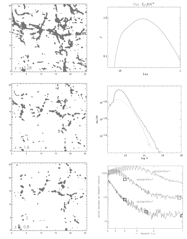
Fig. 9.—: Left handside panels: 25$\times$25$\times$2 Mpc³ slice through the simulation box at $z$ = 3.28, 1.6 and 0.8; contours delineate regions where $N$(H i) $>$ 10¹⁴ cm^-2. Right handside panels: Evolution of the ionizing UV-background flux (calculated from the amount of gas cooling below 5000 K in the simulation); H i column density distribution at $z$ $\sim$ 2; number density of lines with $N$(H i) $>$ 10¹², 10¹³ and 10¹⁴ cm^-2 versus redshift (observational points are overplotted as squares; note the low redshift points from [90]). The simulation is from Riediger et al. [75].

4 METAL LINE SYSTEMS AND GALAXIES

Detailed studies of the kinematics and metallicities of metal line systems (see e.g. [84, 85, 61, 62]) are unique for understanding the structure and evolution of galactic haloes. Indeed the connection between apparently normal galaxies and strong metal absorption line systems has been explored in some detail recently [4, 87, 30]. The fields of quasars known to have metal absorption line systems at $z_{\rm abs}$ are searched for galaxies at redshift $z_{\rm em}$ $\sim$ $z_{\rm abs}$. Up to $z$ $\sim$ 1, there is always such a galaxy within $\sim$ 10 arcsec from the line of sight to the quasar.

At intermediate redshift ($z$ $\sim$ 0.7) Mg ii systems with equivalent width $w_{\rm r}$ $>$ 0.3 Å  are primarily associated with large $R$ $\sim$ 35$h^{-1}$ kpc haloes of a population of luminous ($\sim$$L_{\rm B}^{*}$) galaxies which appear not to evolve significantly over the observed redshift range. The origin, structure and evolution of these large galactic haloes play an important role for the formation and evolution of galaxies, as there is a close interaction between the disk where most of the stars form and the halo that acts as a reservoir of gas.

The most striking result of these studies is that the only interlopers (galaxies that are close to the line of sight but do not induce absorption in the QSO spectrum) have $L_{\rm K}$ $<$ 0.05 $L^{*}_{\rm K}$. At intermediate redshift, the most important criterion for selecting absorbing galaxies seems therefore to be mass rather than star-formation rate. However, it has been shown that the spectral energy distribution of absorbing galaxies is bluer at higher redshift and that the mean equivalent width of [OII]$\lambda$3727 increases by 40% between $z$ $\sim$ 0.4 and $z$ $\sim$ 0.9 [30]. This suggests that star-formation activity is also an important factor for the presence of large haloes. In any case it seems that the structure of haloes is highly perturbed. In particular, it has been shown that the kinematics of the absorption systems is not correlated with the impact parameter ([13] and Fig. 10). Simple disk or halo models are rejected [11].

It is also still unclear which galaxies are associated with weak ($w_{\rm r}$(Mg ii) $<$ 0.3 Å) metal absorption systems. The characteristic radius of haloes can be estimated from the incidence rate of absorption, assuming that every galaxy is surrounded by a spherical halo with filling factor unity, and that the relation between luminosity and halo radius derived from Mg ii galaxy detection can be extrapolated to small equivalent width. The detection limit for weak metal lines has been pushed to very low values with 10m-class telescopes. Mg ii systems are expected to trace the gas with highest density. The number of Mg ii systems per unit redshift at 0.4 $<$ $z$ $<$ 1.4 with $W_{\rm r}$ $>$ 0.02 Å  is d$N$/d$z$ = 1.74$\pm$0.10 [14]. This is four times larger than the number of Lyman limit systems and corresponds to 5% of the number of Ly$\alpha$ forest lines with $W_{\rm r}$ $>$ 0.1 Å. This implies a halo radius of the order of 63$h^{-1}$ kpc for $L^{*}$ galaxies. This suggests that either normal galaxies are surrounded by huge haloes or that weak systems are associated with a population of dwarf galaxies.

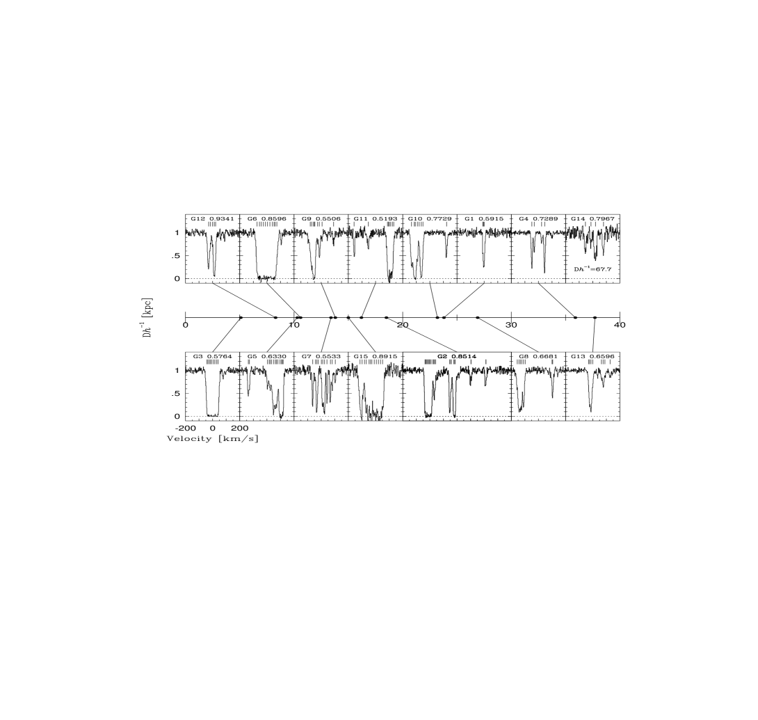
Fig. 10.—: The Mg ii absorption line profiles for ten systems are plotted versus the impact parameter of the field-galaxy closest to the line of sight at the same redshift as the absorber. It is apparent that there is no correlation between the absorption profile and the impact parameter. Although this comparison is very crude since the absorbing galaxies have neither the same luminosity nor the same star-formation rate, this nonetheless suggests that galactic haloes have highly perturbed structures (from Churchill et al. [13]).

5 DAMPED SYSTEMS

Damped Ly$\alpha$ (hereafter DLA) systems are defined as systems with hydrogen column density $N$(H i) $>$ 2$\times$10²⁰ cm^-2. This definition is artificial since damped wings appear for lower column densities ($N$(H i) $>$ 10¹⁹ cm^-2; see Section 2.3 and Fig. 3). It has been introduced assuming that these lines should be characteristic of galactic disks at high redshift [97]. Another reason is that damped Ly$\alpha$ surveys were performed at low resolution. The equivalent width $w_{\rm obs}$($z$ $\sim$ 2.5) $>$ 17.5 Å  for $N$(H i) $>$ 10²⁰ cm^-2. The probability that such a strong absorption feature is the result of blending is small (see Table 3 of [97]). It is clear that this definition may introduce a systematic bias in the discussion of what is the nature of these systems and it would be most valuable to compare the properties of systems with 19 $<$ log $N$(H i) $<$ 20.3 and log $N$(H i) $>$ 20.3.

For log $N$(H i) $>$ 19, the optical depth at the Lyman limit is large enough so that hydrogen is neutral. The gas is either cold ($T$ $<$ 1000 K) and contains molecules (e.g. [83]) or warm ($T$ $\sim$ 10⁴ K) for the highest or lowest column densities respectively [63]. As a consequence of the shape of the column density distribution, d²$n$/d$N$d$z$ $\propto$ $N^{-\beta}$ with $\beta$ $\sim$ 1.5, most of the mass is in the systems of highest column densities. The number density of the latter decreases with time presumably as a consequence of star-formation ([97, 42]; see however [91]). Indeed, the cosmic density of neutral hydrogen in DLA absorbers at $z$ $\sim$ 3 is similar to that of stars at the present time [99, 89].

Metallicities and dust content have been derived from zinc and chromium observations [67, 68]. The [Zn/Cr] ratio is an indicator of the presence of dust if it is assumed, that, as in our Galaxy, zinc traces the gaseous abundances whereas chromium is heavily depleted into dust grains (see [49] and [69] for a critical discussion of this assumption). The typical dust-to-gas ratio determined this way is about 1/30 of that in the Milky-Way [68, 95]. This amount of dust could bias the observed number density of DLA systems [24, 7]. Metallicities are of the order of a tenth solar and tend to decrease from $z$ $\sim$ 2 to $z$ $>$ 3 ([69, 7] and Fig. 11). At any redshift however, the scatter is large and it may be hazardous to draw premature conclusions from the small samples available.

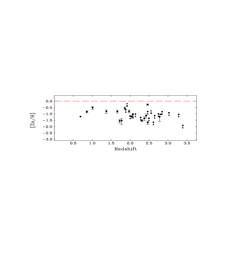
Fig. 11.—: Zinc metallicity (relative to solar) in damped systems versus redshift (from Pettini et al. [69]).

Recently, Prochaska & Wolfe [71] have used Keck spectra of 17 DLA absorbers to investigate the kinematics of the neutral gas from unsaturated low-excitation transitions such as Si ii$\lambda$1808. They show that the absorption profiles are inconsistent with models of galactic haloes with random motions, spherically infalling gas and slowly rotating hot disks. The CDM model [39] is rejected as it produces disks with rotation velocities too small to account for the large observed velocity broadening of the absorption lines. Models of thick disks ($h$ $\sim$ 0.3$R$, where $h$ is the vertical scale and $R$ the radius) with large rotational velocity ($v$ $\sim$ 225 km s^-1) can reproduce the data. In a subsequent paper however, Haehnelt et al. [32] use hydrodynamic simulations in the framework of a standard CDM cosmogony to demonstrate that the absorption profiles can be reproduced by a mixture of rotational and random motions in merging protogalactic clumps. The typical virial velocity of the haloes is about 100 km s^-1.

The issue of whether DLA systems originate in thick disks has been questioned previously. In particular, the metallicity distribution of DLA systems is inconsistent with that of stars in the thick disk of our Galaxy ([69]; see however [100]). Arguments in favor of DLA systems being associated with dwarf galaxies have been reviewed by Vladilo [95]. However, it has been shown recently that DLA systems at intermediate redshift are associated with galaxies of very different morphologies [44]. This strongly suggests that the objects associated with high-redshift DLA absorbers are progenitors of present-day galaxies of all kinds (see [45]).

6 CONCLUSION

The amount of information derived from studies of QSO absorption line systems has increased tremendously during the last few years. This largely results from the improvements in instrumental sensitivity, and spectral resolution and the extension of the accessible wavelength range. Coupled with the development of sophisticated $N$-body simulations, this progress has favored the emergence of a consistent picture in which not only the intergalactic medium is the baryonic reservoir for galaxy formation but also galaxy formation strongly influences the evolution of the IGM through metal enrichment and ionizing radiation emission.

One of the most exciting projects for the next few years may be to probe the 3D spatial distribution of the gas at high redshift. A number of large surveys are underway or planed, which will provide a large number of bright ($m_{\rm V}$ $<$ 19) quasars for investigation of large scales. A few small fields will be searched for deeper samples of quasars ($m_{\rm V}$ $<$ 23). If a hundred lines of sight can be observed in one square degree, the probability distribution function of the matter density could be investigated at high redshift. This would be a unique way to study how galaxy formation is related to the distribution and dynamics of the underlying matter field.

References

- [1] Bajtlik S., Duncan R.C., Ostriker J.P., 1988, ApJ 327, 570.
- [2] Bechtold J., 1994, ApJS 91, 1.
- [3] Bechtold J., Crotts A.P.S., Duncan R.C., Fang Y., 1994, ApJ 437, L83.
- [4] Bergeron J., Boissé, P., 1991, A&A 243, 344.
- [5] Bi HongGuang, Davidsen A.F., 1997, ApJ 479, 523.
- [6] Black J.H., 1981, MNRAS 197, 553.
- [7] Boissé P., Le Brun V., Bergeron J., Deharveng J.M., 1998, A&A 333, 841.
- [8] Burles S., Tytler D., 1998, ApJ 499, 699.
- [9] Carswell R.F., Webb J.K., Cooke A.J., Irwin M.J., 1992, VPFIT Manual (program and manual available from rfc@ast.cam.ac.uk).
- [10] Cen R., Miralda-Escudé J., Ostriker J.P., Rauch M., 1994, ApJ 437, L9.
- [11] Charlton J.C., Churchill C.W., 1998, ApJ 499, 181.
- [12] Charlton J.C., Salpeter E.E., Linder S.M., 1994, ApJ 430, 29.
- [13] Churchill C.W., et al., 1996, ApJ 471, 164.
- [14] Churchill C.W., et al., 1998, astro-ph/9807131.
- [15] Cooke A.J., Espey B., Carswell R.F., 1997, MNRAS 284, 552.
- [16] Cowie L.L., Songaila A., Kim T-S, Hu E.M., 1995, AJ 109, 1522.
- [17] Cowie L.L., Songaila A., 1998, Nature 394, 44.
- [18] Cristiani S., et al., 1997, MNRAS 285, 209.
- [19] Croft R.A.C., Weinberg D.H., Katz N., Hernquist L., 1998, ApJ 495, 44.
- [20] Crotts A.P.S., Fang Y., 1998, ApJ 502, 16.
- [21] Dinshaw N., Weymann R.J., Impey C.D., Foltz C.B., Morris S.L., Ake T., 1998, ApJ 494, 567.
- [22] D’Odorico V., et al., 1998, A&A 339, 678.
- [23] Espey B.R., 1993. ApJ 411, L59.
- [24] Fall S.M., Pei Y.C., 1993, ApJ 402, 479.
- [25] Fardal M.A., Giroux M.L., Shull J.M., 1998, AJ 115, 2206.
- [26] Fernandez-Soto A., et al., 1996, ApJ 460, L85.
- [27] Fontana A., Ballester P., 1995, The Messenger 80, 37.
- [28] Fukugita M., Lahav O., 1991, MNRAS 253, 17P.
- [29] Giallongo E., Fontana A., Cristiani S., D’Odorico S., 1998, astro-ph/9809258.
- [30] Guillemin P., Bergeron J., 1997, A&A 328,499.
- [31] Haardt F., Madau P., 1996, ApJ 461, 20.
- [32] Haehnelt M.G., Steinmetz M., Rauch M., 1998, ApJ 495, 647.
- [33] Hamann F., 1997, ApJS 109, 279.
- [34] Hernquist L., Katz N., Weinberg D.H., Miralda-Escudé J., 1996, ApJ 457, L51.
- [35] Hu E.M., Kim T-S, Cowie L.L., Songaila A., Rauch M., 1995, AJ 110, 1526.
- [36] Ikeuchi S., Ostriker J.P., 1986, ApJ 301, 522.
- [37] Impey C.D., Foltz C.B., Petry C.E., Browne I.W.A., Patnaik A.R., 1996, ApJ 462, L53.
- [38] Jannuzi B., et al., 1998, ApJS 118, 1.
- [39] Kauffmann G., 1996, MNRAS 281, 475.
- [40] Kim T.S., Hu E.M., Cowie L.L., Songaila A., 1997, AJ 114, 1.
- [41] Kulkarni V.P., Fall S.M., 1995, ApJ 453, 55.
- [42] Lanzetta K.M., Wolfe A.M., Turnshek D.A., 1995, ApJ 440, 435.
- [43] Lanzetta K.M., 1998, in Evolution and Structure of the IGM, XIII IAP colloquium, eds P. Petitjean & S. Charlot, Editions Frontières, p. 213.
- [44] Le Brun V., Bergeron J., Boissé P., Deharveng J.M., 1997, A&A 321, 733.
- [45] Ledoux C., Petitjean P., Bergeron J., Wampler E.J., Srianand R., 1998, A&A 337, 51.
- [46] Lespine Y., Petitjean P., 1997, A&A 317, 416.
- [47] Levshakov S.A., Kegel W.H., 1997, MNRAS 288, 787.
- [48] Levshakov S.A., Kegel W.H., Takahara F., 1998, ApJ 499, L1.
- [49] Lu L., Sargent W.L.W., Barlow T.A., Churchill C.W., Vogt S.S., 1996, ApJS 107, 475.
- [50] Lu L., Sargent W.L.W., Barlow T.A., Rauch M., 1998, astro-ph/9802189.
- [51] Mar D., 1994, Xvoigt User’s Guide, mar@physics.su.oz.au.
- [52] Meiksin A., Madau P., 1993, ApJ 412, 34.
- [53] Miralda-Escudé J., Ostriker J.P., 1990, ApJ 350, 1.
- [54] Miralda-Escudé J., Cen R., Ostriker J.P., Rauch M., 1996, ApJ 471, 582.
- [55] Miralda-Escudé J., Rees M.J., 1997, ApJ 478, L57.
- [56] Morton D.C., Smith W.H., 1973, ApJS 26, 333.
- [57] Morton D.C., York D.G., Jenkins E.B., 1988, ApJS 68, 449.
- [58] Mücket J.P., Petitjean P., Kates R., Riediger R., 1996, A&A 308, 17.
- [59] Nusser A., Haehnelt M., 1998, astro-ph/9806109.
- [60] Petitjean P., 1997, in The Early Universe with the VLT, ed. J. Bergeron, ESO Workshop, Springer, p.266.
- [61] Petitjean P., Bergeron J., 1990, A&A 231, 309.
- [62] Petitjean P., Bergeron J., 1994, A&A 283, 759.
- [63] Petitjean P., Bergeron J., Puget J.L., 1992, A&A 265, 375.
- [64] Petitjean P., Mücket J.P., Kates R.E., 1995, A&A 295, L9.
- [65] Petitjean P., et al., 1998, A&A 334, L45.
- [66] Petitjean P., Webb J.K., Rauch M., Carswell R.F., Lanzetta K., 1993, MNRAS 262, 499.
- [67] Pettini M., Smith L.J., Hunstead R.W., King D.L., 1994, ApJ 426, 79.
- [68] Pettini M., King D.L., Smith L.J., Hunstead R.W., 1997a, ApJ 478, 536.
- [69] Pettini M., Smith L.J., King D.L., Hunstead R.W., 1997b, ApJ 486, 665.
- [70] Press W.H., Rybicki G.B., 1993, ApJ 418, 585.
- [71] Prochaska J.X., Wolfe A.M., 1997, ApJ 474, 140.
- [72] Rauch M., et al., 1997, ApJ 489, 7.
- [73] Rauch M., 1998, ARA&A Vol. 36, astro-ph/9806286.
- [74] Rees M.J., 1986, MNRAS 218, 25P.
- [75] Riediger R., Petitjean P., Mücket J.P., 1998, A&A 329, 30.
- [76] Sargent W.L.W., Young P.J., Boksenberg A., Tytler D., 1980, ApJS 42, 41.
- [77] Savage B.D., Sembach K.R., 1996, ARA&A 34, 279.
- [78] Schneider D.P., Schmidt M., Gunn J.E., 1991, AJ 102, 837.
- [79] Smette A., et al., 1995, A&AS 113, 199.
- [80] Songaila A., 1998, astro-ph/9803010.
- [81] Songaila A., Cowie L.L., 1996, AJ 112, 335.
- [82] Songaila A., et al., 1994, Nature 371, 43.
- [83] Srianand R., Petitjean P., 1998, A&A 335, 33.
- [84] Steidel C.C., 1990, ApJS 72, 1.
- [85] Steidel C.C., 1990, ApJS 74, 37.
- [86] Steidel C.C., 1993, J.M. Shull and H.A. Thronson Jr. (eds) Proc. of the Third Tetons Summer School,The Environment and Evolution of Galaxies, Kluwer, Dordrecht, p. 263.
- [87] Steidel et al. 1994 ApJ 437, L75.
- [88] Steidel C.C., 1998, ApJ 492, 428.
- [89] Storrie-Lombardi L.J., McMahon R.G., Irwin M.J., 1996, MNRAS 283, L79.
- [90] Tripp T.M., Lu L., Savage B.D., 1998, astro-ph/9806036.
- [91] Turnshek D.A., 1998, in Evolution and Structure of the IGM, XIII IAP colloquium, eds P. Petitjean & S. Charlot, Editions Frontières, p. 263.
- [92] Turnshek D.A., et al., 1996, ApJ 463, 110.
- [93] Tytler D., et al., 1995, in QSO Asorption Lines, ESO Workshop, G. Meylan (ed.), Heidelberg, Springer, p. 289.
- [94] Verner D.A., Barthel P.D., Tytler D., 1994, A&AS 108, 287
- [95] Vladilo G., 1998, ApJ 493, 583.
- [96] Wampler E.J., Chugai N.N., Petitjean P., 1995, ApJ 443, 586.
- [97] Wolfe A.M., et al., 1986, ApJS 61, 249.
- [98] Wolfe A., 1988. In Blades J.C., Turnshek D.A., Norman C.A. (eds) Proc. Workshop, QSO Absorbing Lines: Probing the Universe. Cambridge University Press, Cambridge, p. 297.
- [99] Wolfe A.M., 1995, in QSO Absorption Lines, ed. G. Meylan (Berlin: Springer), 13.
- [100] Wolfe A.M., Prochaska J.X., 1998, ApJ 494, L15.
- [101] Zhang Y., Meiksin A., Anninos P., Norman M.L., 1998, ApJ 495, 63.