A New Approximation Of ECM Frequencies

Abstract

We investigate wave amplification through the Electron Cyclotron Maser mechanism. We derive a semi-analytic approximation formula giving the frequencies at which the absorption coefficient is negative. The coefficients still need to be computed to obtain the largest, and therefore the dominant, coefficient.

1 Introduction

The observation of millisecond microwave spikes from the Sun has been interpreted as gyrosynchrotron maser emission since the late 1970‘s (Wu ; Holman ). The spikes exhibit a duration of a few milliseconds to some tens of milliseconds, and a narrow bandwidth ($\approx 1\%$ or a few MHz). The characteristic high brightness temperature ($10^{15-18}\ K$) deduced for the spikes strongly suggests maser action (BenzBook ).

Several papers have explored the possibilities of cyclotron maser. Melrose and Dulk (D+M ) have used the semi-relativistic approximation to derive approximate formulae for the frequency of the largest growth rate, and for the growth rate. Winglee (Winglee ) approximated the effects of the ambient plasma temperature on the maser emission. Aschwanden (Aschwanden a , Aschwanden b ) followed the diffusion of electrons into the loss-cone as a result of the maser emission, and therefore the self-consistent closure of the loss-cone as the energy is transferred to the maser. Kuncic and Robinson (Kuncic ) performed ray-tracing in a model loop with dipole field, and concluded that maser emission can escape from lower levels.

Some papers have also attempted to derive analytical approximate formulae for the frequencies of the maser. Dulk and Melrose (D+M ) concluded that the maser emission is at, or near, $90$ degrees to the magnetic field and the maximum growth rate they find is very near the cyclotron frequency, or at the second harmonic. Hewitt and Melrose (Hewitt ) derive the conditions for solutions and the number of solutions, but not the frequencies themselves.

All previous studies concentrated on the growth rate of the amplified wave, we use the absorption coefficient approach of Ramaty (R ) and calculate the frequencies at which the absorption coefficient is negative.

2 Gyrosynchrotron Absorption

In studies of microwave emission from solar flares it is customary to assume that the plasma is composed a non-thermal population of energetic elecrons, and a thermal population of much higher density, but much lower energy. The thermal plasma is assumed to determines the propagation of waves. This plasma can be described by the cold plasma approximation using magnetoionic theory (MelroseB ).

ECM studies usually compute the growth rate, while we follow Ramaty (R ) in using the absorption coefficient, but for the purposes of this article the detailed equations are unimportant. Both the growth rate equation and the absorption coefficient equation include a $\delta$-function from which the important resonance condition is derived

$${{s\omega_{B}}\over\gamma}=\omega(1-n_{\pm}\beta\cos(\theta)\cos(\phi))$$ (1)

where $\omega_{B}=eB/m_{e}/c$ is the cyclotron frequency, $\omega$ is the emission frequency, $s$ is an integer, $\theta$ is the angle of the wave vector ${\bf k}$ to the magnetic field, $\phi$ is the angle between the velocity of the electron and the magnetic field (the pitch angle), and $\gamma$ and $\beta$ are the usual Lorentz factor and velocity. The important factor in equation 1 is $n_{\pm}$ the refraction index for the Ordinary Mode (OM or ’+’), and the eXtra-Ordinary mode (XO or ’-’). The refraction index is a function of the ambient density, of the cyclotron frequency, of the emission frequency, and of the angle to the magnetic field

$$n_{\pm}^{2}= 1+$$

$${{2\nu_{p}^{2}(\nu_{p}^{2}-\nu^{2})}\over{-2\nu^{2}(\nu_{p}^{2}-\nu^{2})-\nu^{2}\nu_{B}^{2}\sin^{2}(\theta)\pm\sqrt{\Delta}}}$$

$$\Delta=\nu^{4}\nu_{B}^{4}\sin^{4}(\theta)+4\nu^{2}\nu_{B}^{2}(\nu_{p}^{2}-\nu^{2})^{2}\cos^{2}(\theta)$$

Where $\nu_{p}$ is the plasma frequency and the rest are as in equation 1.

If $\theta\neq\pi/2$ the $\delta$ function is transformed to

$$\delta\left(\nu-{{s\nu_{B}}\over{\gamma}}-n_{\pm}\nu\beta\cos(\phi)\cos(\theta)\right)=$$ (3)

$$\delta\left(\cos(\phi)-{{1-{{s\nu_{B}}\over{\gamma\nu}}}\over{n_{\pm}\beta\cos(\theta)}}\right){{1}\over{n_{\pm}\nu\beta\cos(\theta)}}$$

This transformation gives us the pitch angle $\phi_{s}$ of an electron emitting in direction $\theta$ a wave of frequency $\nu$, where

$$\cos(\phi_{s})={{1-{{s\nu_{B}}\over{\gamma\nu}}}\over{n_{\pm}\cos(\theta)\beta}}$$ (4)

The absorption coefficient after the integration over the pitch angle is (R )

$$k_{\pm}\left({\nu,\theta}\right)={1\over B}4\pi^{2}e{{2\pi}\over{\left|\cos\left(\theta\right)\right|}}{{\nu_{B}}\over\nu}{1\over{n_{\pm}^{2}}}\times$$ (5)

$$\int_{1}^{\infty}d\gamma{{u\left(\gamma\right)}\over\beta}\sum\limits_{s=s_{1}}^{s_{2}}{{g\left({\phi_{s}}\right)}\over{1+T_{\pm}^{2}}}\Bigl{[}\beta\sin\left({\phi_{s}}\right)J_{s}^{\prime}\left({x_{s}}\right)+$$

$${{L_{\pm}}\over{n_{\pm}}}J_{s}\left(x_{s}\right)+T_{\pm}\left({{\cot\left(\theta\right)}\over{n_{\pm}}}-{{\beta\cos\left({\phi_{s}}\right)}\over{\sin\left(\theta\right)}}\right)J_{s}\left({x_{s}}\right)\Bigr{]}^{2}\times$$

$$\Bigl{[}{{-\beta\gamma^{2}}\over{u\left(\gamma\right)}}{d\over{d\gamma}}{{u\left(\gamma\right)}\over{\beta\gamma^{2}}}+{{n_{\pm}\beta\cos\left(\theta\right)-\cos\left({\phi_{s}}\right)}\over{\gamma\beta^{2}\sin\left({\phi_{s}}\right)}}\times$$

$${1\over{g\left({\phi_{s}}\right)}}{{dg\left(\phi\right)}\over{d\phi}}\Bigr{]}$$

Where $J_{s}$ are Bessel functions, with the argument $x_{s}=(\nu/\nu_{B})n_{\pm}\gamma\beta\sin(\theta)\sin(\phi)$. The cold plasma parameter $T_{\pm}$ is the ratio of the polarization ellipse axis, which describes the transverse part of the polarization vector, and the parameter $L_{\pm}$ describes the longitudinal part of the polarization vector. Equations for $T_{\pm}$ and $L_{\pm}$ can be found in Melrose (MelroseB ). The range of the summation over the Bessel functions is

$$s_{1,2}={{\nu\gamma}\over{\nu_{B}}}\left(1\pm n_{\pm}\beta\cos(\theta)\right)$$ (6)

And $u(\gamma)g(\phi)$ is the distribution function of the emitting electrons.

We assume the distribution function in equation 5 can be put in the form

$$f({\bf p})d^{3}p=2\pi u(\gamma)g(\phi)d\gamma d(\cos(\phi))$$

And take for the distribution function of the non-thermal electrons a power-law

$$u(\gamma)=A\cdot(\gamma-1)^{-\delta}$$ (7)

which is normalized to $n_{hot}$ the number density of the energetic electrons. For the pitch angle dependence in the energetic distribution we use an ideal loss-cone which describes an isotropic distribution for pitch angles above some $\alpha$, no electrons below another angle $\alpha-\Delta\alpha$, and a linear in $cos(\phi)$ decrease within the $\Delta\alpha$ interval (D+M ), or :

$$g(\phi)=\cases{A,&$\cos(\phi)<\cos(\alpha)$\cr A\times{{cos(\alpha-\Delta\alpha)-cos(\phi)}\over{cos(\alpha-\Delta\alpha)-\cos(\alpha)}},&$\cos(\alpha)<\cos(\phi)<$\cr&$cos(\alpha-\Delta\alpha)$\cr 0,&$cos(\alpha-\Delta\alpha)<\cos(\phi)$\cr}$$ (8)

Where $A$ is a constant which depends on the loss cone parameters, and for an idealized loss cone as above is $A=1/\pi/(2+\cos(\alpha)+cos(\alpha-\Delta\alpha))$. With this constant the integral is normalized so that $2\pi\int_{-1}^{1}g(\phi)d(\cos\phi)=1$.

3 Conditions for Maser

The Electron-Cyclotron-Maser occurs when the absorption coefficient is negative. The resulting amplification of the radiation is referred to as maser.

Inspection of equation 5 shows that the absorption coefficient for a distribution which is isotropic in pitch angle can only be negative if the slope of $u(\gamma)/\gamma^{2}/\beta$ is positive. This is the equivalent of an increase of the fast particles with energy, a distribution which is not likely to occur. The other possibility for amplification is when the distribution is not isotropic in pitch angle. In that case if the derivative of $g(\phi)$ is large enough, and there are solutions such that the pitch angle dependent term in equation 5 is negative, then the absorption will be negative. One such anisotropic distribution is the loss-cone distribution, which we use. The loss-cone distribution produces negative absorption coefficients and maser emission.

4 Semi-Analytical Formulae

The resonance condition 1 defines an ellipse on the electron velocity plane $(v_{||},v_{\perp})$ for a given $s$,$\theta$, and frequency of emission (MelroseB ). The integral over the electron distribution function, which is necessary to calculate the absorption coefficient, is therefore an integral along the ellipses of the various $s$ harmonics. In the weakly relativistic case $1/\gamma=1-\beta^{2}/2$ this ellipse becomes a circle (D+M ) - the resonance circle - whose center is on the $v_{||}$-axis (the x-axis) at $v_{||}=v_{c}$, and whose radius is $v_{R}$ with

$${{v_{c}}\over{c}}={{n_{\pm}\cos(\theta)\nu}\over{s\nu_{B}}}$$ (9)

$${{v_{R}}\over{c}}=\sqrt{\left({{v_{c}}\over c}\right)^{2}-{{2(\nu-s\nu_{B})}\over{s\nu_{B}}}}$$ (10)

The loss-cone described by equation 8 divides the $(v_{||},v_{\perp})$ plane into three regions. Below the line of angle $\alpha-\Delta\alpha$ to the $v_{||}$-axis there are no electrons, above the line of angle $\alpha$ to the $v_{||}$-axis the distribution is isotropic in angle, and between the two lines the number density of electrons decreases with angle.

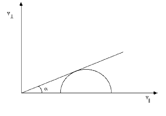
Figure 1: A loss-cone on the plane $(v_{||},v_{\perp})$ is a straight line with angle $\alpha$ to the x-axis. The resonance condition defines, with the small $\gamma$ approximation, a resonance circle on the plane. The special circle which is tangent to the line of the loss-cone is the circle for the frequency where the largest in absolute value negative absorption occurs.

The frequency and angle for which the largest (in absolute value) negative absorption is expected are those for which the resonance circle is tangent to the outer edge of the loss-cone at $\alpha$ (D+M ), as shown in figure 1. Integration along this special circle passes only through the two lower regions where there are either no electrons, or the distribution changes with angle. Where there are no electrons the absorption is zero, and where the distribution changes with angle is where the integrand is most likely to be negative, and therefore integration around the special circle is the most likely to give negative absorption. The special circle also has the longest possible path through this region, and is expected to produce the largest (in absolute value) negative absorption coefficient.

The definition of the special circle results in an equation for a frequency which is the frequency where the largest absorption is expected. This frequency is (D+M )

$${\nu\over{\nu_{B}}}=s\left(1+{{n_{\pm}^{2}\cos^{2}(\theta)\cos^{2}(\alpha)}\over 2}\right)$$ (11)

Since even a short path through the positively contributing region of the $(v_{||},v_{\perp})$ plane increases the positive absorption considerably, the expectation is that there are negative absorption coefficients only for this special frequency, or at frequencies very close to it.

For the fully relativistic case it is more convenient to consider the plane $(\gamma,\cos(\phi))$. On this plane the loss cone regions are the region below the line parallel to the $\gamma$-axis (the $x$-axis) at $\cos(\phi)=\cos(\alpha-\Delta\alpha)$, where the number density is independent of the pitch angle, the region above the line $\cos(\phi)=\cos(\alpha)$, where there are no electrons, and the region between the lines, where the number density decreases. On the $(\gamma,\cos(\phi))$ plane the resonance condition defines a curve which is given by equation 4.

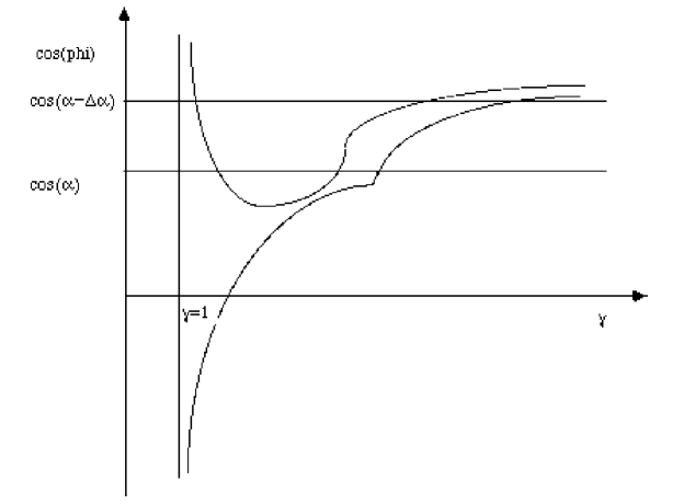
Figure 2: On the plane $(\gamma,\cos(\phi))$ the solution of the resonance condition for the pitch angle (equation 4) can appear in one of two forms. The first curve goes to $+\infty$ when $\gamma$ approaches $1$ from above, and the second curve goes to $-\infty$ when $\gamma$ approaches $1$. For some frequency the first form is tangent to the $\cos(\phi)=\cos(\alpha)$ outer edge of the loss-cone, and this curve has the largest in absolute value negative absorption coefficient.

There are two possible forms to the curve given by equation 4, as shown in figure 2. The first form is for $s\nu_{B}>\nu$. For this case, as $\gamma$ approaches $1$ from above, and assuming $\cos(\theta)>0$, the $\cos(\phi_{s})$ solution goes to minus infinity. The second form of the curve is for $s\nu_{B}<\nu$, and for this form the $\cos(\phi_{s})$ solution goes to positive infinity as the kinetic energy approaches zero. Both curves go asymptotically to $[n_{\pm}\cos(\theta)]^{-1}$ as $\gamma$ goes to infinity. The second form curve (for $\nu>s\nu_{B}$) undergoes a change in the sign of the slope at some energy. For that curve the value of $\cos(\phi_{s})$ ceases to decrease as $\gamma$ increases (negative slope), and starts to increase (positive slope), as figure 2 illustrates.

For the fully relativistic case the equivalent curve to the special resonance circle is a curve with the second form, which on the $(\gamma,\cos(\phi))$ plane is tangent to the line $\cos(\phi)=\cos(\alpha)$. This curve goes only through the two upper regions of the plane, where there are either no electrons, or the density is pitch angle dependent - where the integrand in equation 5 is most likely to be negative. This special curve also has the longest possible path through the negative contribution region, and therefore the absorption coefficient derived from integration along this curve should be the largest negative absorption coefficient possible. The turnover of the special curve is at energy

$$\gamma=\nu/(s\nu_{B})$$ (12)

and the frequency which gives this curve is given by the equation

$${\nu\over{\nu_{B}}}={s\over\sqrt{1-n_{\pm}^{2}\cos^{2}(\theta)\cos^{2}(\alpha)}}$$ (13)

The equation 13 is our new approximation. Our approximation becomes identical with the Melrose and Dulk approximation 11 for the case $n_{\pm}^{2}\cos^{2}(\theta)\cos^{2}(\alpha)<<1$. It is, however, more general and is a good approximation for the frequencies of negative absorption, even when $n_{\pm}^{2}\cos^{2}(\theta)\cos^{2}(\alpha)$ is large, as the examples in section 6 demonstrate.

Even though we utilize the approximation 13 it is important to note that it is also possible for a curve of the first form, with $s\nu_{B}>\nu$, to give a negative absorption coefficient. This may occur if the curve reaches $\cos(\phi)=\cos(\alpha)$ for an energy which is close to the low-energy cut-off of the fast electron distribution. For this case most of the curve at $\cos(\phi)<\cos(\alpha)$ is at energies where there are no fast electrons. This part of the curve therefore has no contribution to the absorption coefficient, and since this is the region where the positive contribution comes from, the resulting absorption is negative. We used in our calculations a low-energy cut-off of $\gamma_{min}=1.02$, which is a common assumption. It turns out that it is very unlikely that equation 4 gives $\cos(\phi_{s})=\cos(\alpha)$ for an energy lower or close to this cut-off. The equation 13 therefore gives most of the solutions, and can be used to find the frequencies of negative absorption.

Equation 13 is still an approximation, and in deriving it we made simplifying assumptions . For example frequencies close to the special frequency given by equation 13 also have negative absorption, because as long as the curve for some frequency has a short path through the isotropic region the absorption can remain negative. Equation 13 also assumes a single harmonic $s$ while the absorption coefficient equation 5 includes a sum over all harmonics from $s_{1}$ to $s_{2}$. The positive contribution of other harmonics moves the negative absorption towards zero, and can not be easily approximated. Therefore the frequency with largest negative absorption is usually not exactly the solution of equation 13, but a frequency close to it.

A close look at equation 13 shows that it must be solved numerically, because the refraction index $n_{\pm}$ is a function of the frequency $\nu$. The refraction index is where the ratio between the plasma frequency $\nu_{p}$ and the cyclotron frequency $\nu_{B}$ comes into play, since it is very sensitive to this ratio for low multiples of $\nu_{B}$. Our approximation is therefore only semi-analytical, since some numerical computation must be made. The computation, however, is very simple and can be performed very quickly.

There are some general properties of the solutions it is possible to derive even without calculation of the refraction index, and we proceed to do so in the next section.

Finally, equation 13 was derived with the assumption that $\cos(\theta)>0$, but if $\cos(\theta)<0$ then $\cos(\alpha)<0$ as well, and the solution is the same. Equation 13 can therefore be used for all cases.

5 General Properties of the Solution

The first general property of the solution given in equation 13 is the requirement that $\nu>s\nu_{B}$. This may not always be the case (as shown in the previous section), but it turns out that this condition holds for the dominant (defined as the most strongly amplified) modes. In practical terms this condition sets the appearance of negative absorption at frequencies between $s\nu_{B}$ and $(s+0.5)\nu_{B}$.

Other general properties can be demonstrated by a graphical solution of equation 13. On a plane where the x-axis are the frequency we plot the line $y=\nu$, and the function

$$f(\nu)={{s\nu_{B}}\over{\sqrt{1-n_{\pm}^{2}\cos^{2}(\theta)\cos^{2}(\alpha)}}}$$ (14)

Any frequency for which the two curves intersect is a solution of equation 13.

There are two special cases for the OM and the XO mode where we can compare $f(\nu)$ and $y=\nu$ without explicitly calculating the refraction index. The first case is at the special points of the cut-off frequencies of the modes,where $n_{\pm}=0$. The second special case is for large frequencies, where the refraction indices are $n_{\pm}=1$. The general shape of the curve 14 can be inferred from these two points.

The OM cut-off is at $\nu=\nu_{p}$, and therefore for the Ordinary Mode $f(\nu_{p})=s\nu_{B}$, and if the plasma frequency is equal to the cyclotron frequency, or some harmonic of the cyclotron frequency, then $\nu_{p}$ is a solution. The XO mode cut-off is at the frequency

$$\nu_{x}=\nu_{B}/2+\sqrt{\nu_{p}^{2}+\nu_{B}^{2}/4}$$ (15)

This cut-off is always at higher frequency than $\nu_{B}$, and therefore $f(\nu_{x})<\nu_{x}$ with $s=1$. However, if $\nu_{p}=\sqrt{2}\nu_{B}$ then the cut-off is at $\nu_{x}=2\nu_{B}$, and the second harmonic $s=2$ is a solution. For any harmonic $s$, the cut-off frequency is equal to $s\nu_{B}$ for a ratio $(\nu_{p}/\nu_{B})^{2}=s^{2}-s$.

The cut-off frequencies of the modes are not important themselves, because a wave with a zero refraction index can not propagate. However, the solutions can be used to deduce the behaviour of the curve 14. The line $y=\nu$ and the curve 14 can have one of two relations at the cut-off frequencies :

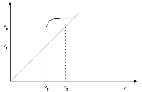
Figure 3: A depiction of the plot for $f(\nu)$ (equation 14) for the OM, and the case $\nu_{B}>\nu_{p}$. The curve begins above the line $y=\nu$, and there is only one possible intersection, and therefore only one possible solution of equation 13.

• If the plasma frequency is smaller than the cyclotron frequency then $f(\nu_{p})=\nu_{B}>\nu_{p}$ and the curve 14 for the OM starts above the $y=\nu$ line (figure 3). More generally, for all harmonics $s$ such that $s\nu_{B}>\nu_{p}$ the curve for the OM starts above the $y=\nu$ line.

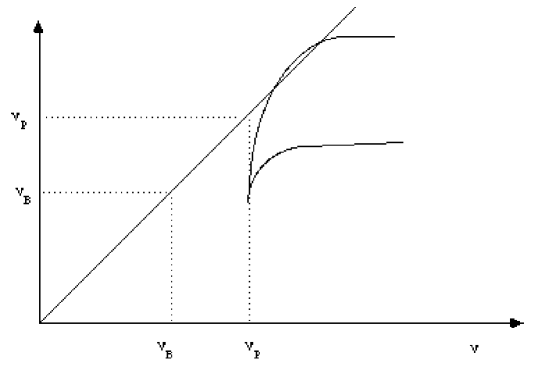
Figure 4: A depiction of the plot for $f(\nu)$ (equation 14) for the OM, and the case $\nu_{B}<\nu_{p}$. The curve begins below the line $y=\nu$, and therefore there may be no solution, or there are two solutions of equation 13.

• Conversely, if the plasma frequency is larger than some harmonic $m$ of the cyclotron frequency, then the OM curve 14 starts below the $y=\nu$ line for $s$ up to and including the harmonic $m$ (figure 4).

• If $(\nu_{p}/\nu_{B})^{2}<s^{2}-s$, then $f(\nu_{x})=s\nu_{B}>\nu_{x}$, and the curve 14 for the XO starts above the line $y=\nu$. because then $\nu_{x}<s\nu_{B}$.

• If $(\nu_{p}/\nu_{B})^{2}>s^{2}-s$, then the XO curve starts below the line $y=\nu$.

The behaviour of the curve 14 for frequencies larger than the cut-off frequencies is deduced from the refraction index. Both the OM and the XO mode have refraction indices smaller than $1$ which approach $1$ asymptotically as the frequency increases. A curve like the curve 14 therefore has the shape illustrated in figure 3 if it starts above $y=\nu$. From figure 3 it is seen that for a starting point above the $y=\nu$ line there is only one intersection. If the curve starts below the $y=\nu$ line there are either two intersections, or no intersection at all, as is illustrated in figure 4. The conclusion is that for the OM there is one solution for negative absorption coefficients if $s\nu_{B}>\nu_{p}$, and for the XO there is one solution if $\sqrt{s^{2}-s}\ \nu_{B}>\nu_{p}$. There are either two solutions or no solution for the OM if $s\nu_{B}<\nu_{p}$, and for the XO there are two solutions or no solution if $\sqrt{s^{2}-s}\ \nu_{B}<\nu_{p}$. In practice for the cases where the curve 14 starts below the $y=\nu$ line, there is usually no solution, and only the case illustrated in figure 3 is important.

There is an additional limit we can derive from equation 13. The mathematical formula derived in equation 14 can be plotted as a function of frequency for any frequency. However, beyond some frequency the mathematical result $f(\nu)$ is no longer relevant to finding the negative absorption coefficient. The most important limit is derived from equation 14 itself, and it is the highest frequency possible for a given harmonic $s$ with this equation. Clearly, plotting $f(\nu)$ beyond this frequency is meaningless. The highest possible frequency is derived for the OM and the XO by assuming that $n_{\pm}=1$, and is therefore :

$$\nu_{max}={{s\nu_{B}}\over\sqrt{1-\cos^{2}(\theta)\cos^{2}(\alpha)}}$$ (16)

For example with $\cos(\alpha)=0.8$, $s=1$, and emission direction $\cos(\theta)=0.3$ the upper limit on the frequencies usable for this set of parameters is $\nu<1.03\nu_{B}$. If we take $\cos(\theta)=0.7$ the limit is $\nu<1.207\nu_{B}$. This result gives the range of frequencies where negative absorption is expected. For example, $\cos(\theta)=0.3$ can only have negative absorption between $\nu=\nu_{B}$ and $\nu=1.03\nu_{B}$.

The condition 16 can also be used to limit the harmonics relevant for any frequency and angle of emission. For example the first harmonic $s=1$ is not useful for finding negative absorption coefficients at $\nu>2\nu_{B}$ for any loss-cone with $\cos(\alpha)<0.866$. It is thus possible to immediately disqualify certain harmonics from contributing in certain frequency ranges, and shorten the computation time further.

In summary, we conclude that for the OM and the XO mode, we expect negative absorption coefficient to appear for frequencies obeying the following two conditions :

• For the OM the frequency should be derived from a harmonic $s$ which has $s>\nu_{p}/\nu_{B}$.

• For the XO mode the frequency should be derived from a harmonic $s$ which has $s^{2}-s>(\nu_{p}/\nu_{B})^{2}$.

• For both modes the frequency must be smaller than $\nu_{max}$ of equation 16

The harmonic number $s$ of a frequency can be derived from the condition 16 and should be the smallest integer which fits the inequality

$$s\geq{{\nu}\over{\nu_{B}}}\sqrt{1-\cos^{2}(\theta)\cos^{2}(\alpha)}$$ (17)

The largest harmonic $s$ which contributes to a frequency is given by equation 6, but it is reasonable to assume that the smallest harmonic has the largest contribution, and therefore we can consider it alone for the purposes of the approximation.

So far we have not considered the important Z-mode (ZM). The Z-mode is the lower branch of the XO mode, which reappears at frequencies smaller than $\nu_{z}$

$$2\nu_{z}^{2}=\nu_{B}^{2}+\nu_{p}^{2}+\sqrt{(\nu_{B}^{2}+\nu_{p}^{2})^{2}-4\nu_{B}^{2}\nu_{p}^{2}\cos^{2}(\theta)}$$ (18)

and its cut-off frequency is $\nu_{x}-\nu_{B}$.

Emission in the Z-mode can not emerge from the plasma, and therefore can not be observed. Since our purpose is to derive estimates for the observable frequencies, approximate solutions for the Z-mode are not of great interest to us. However, the Z-mode may be the dominant mode and quench the maser before the other modes are amplified. It is therefore of interest to determine where possible negative frequencies can appear.

The upper Z-mode frequency $\nu_{z}$ is bound from above by the upper hybrid frequency

$$\nu_{uh}=\sqrt{\nu_{p}^{2}+\nu_{B}^{2}}$$ (19)

From the equation it is clear that $\nu_{z}$ decreases with increasing $\cos(\theta)$, and for $\cos(\theta)=1$ the limiting frequency is either $\nu_{z}=\nu_{B}$ if $\nu_{p}<\nu_{B}$ or $\nu_{z}=\nu_{p}$ if $\nu_{p}>\nu_{B}$. The lower frequency boundary of the ZM is always smaller than $\nu_{p}$.

The ZM refraction index is $n_{ref}>1$ for frequencies $\nu>\nu_{p}$, is $n_{ref}=1$ at the plasma frequency, and is smaller than $1$ for frequencies smaller than $\nu_{p}$.

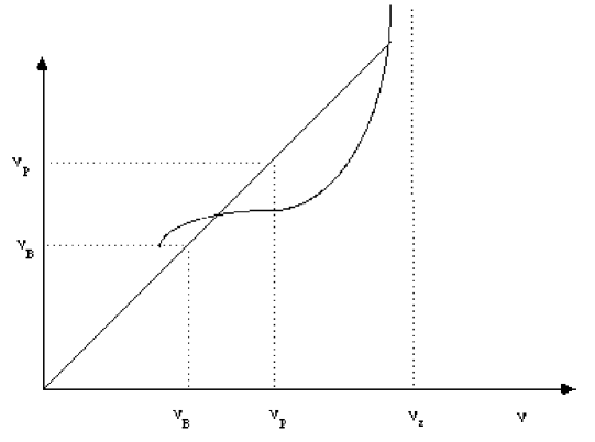
Figure 5: A depiction of the plot for $f(\nu)$ (equation 14) for the ZM, and the case $\nu_{p}>s\nu_{B}/\sqrt{1-\cos^{2}(\theta)\cos^{2}(\alpha)}$. The curve begins below the line $y=\nu$, and therefore there may be one solution for $\nu>\nu_{p}$ or two solutions, one of them for $\nu<\nu_{p}$.

Using the above characteristics we can determine the general behaviour of the curve 14 for the Z-mode, which is illustrated in figure 5. The curve goes to infinity for frequencies near $\nu_{z}$, and goes to $s\nu_{B}$ as the frequency approaches $\nu_{x}-\nu_{B}$.

As for the OM and the XO mode it is possible to deduce the general behaviour of the solutions for the Z-mode from the properties of the refraction index, however, because of the additional dependence on $\cos(\theta)$ the ZM properties are much harder to pin down.

• If $\nu_{p}>\nu_{max}$ (see equation 16), the line $y=\nu$ is above the curve 14 at the plasma frequency. Since the curve 14 goes to infinity near $\nu_{z}$, there is an intersection near $\nu_{z}$, for a frequency $\nu>\nu_{p}$. The effect of $\cos(\theta)$ complicates this condition, which is not just $\nu_{p}>s\nu_{B}$, since for large $\cos(\theta)$ even a high plasma frequency may not be larger than $s\nu_{B}/\sqrt{1-\cos^{2}(\theta)\cos^{2}(\alpha)}$.

• If in addition to the above also $\nu_{x}-\nu_{B}<s\nu_{B}$ then there is also an intersection for $\nu<\nu_{p}$.

• If $\nu_{p}<\nu_{max}$, the line $y=\nu$ is below the line of curve 14 at $\nu_{p}$. If, in addition, $\nu_{p}>s\nu_{B}$, then there is no solution. This condition tells us that there are no ZM solutions for large $\cos(\theta)$.

• If $\nu_{p}<\nu_{max}$, but $\nu_{p}<s\nu_{B}$ than there is no intersection in the range $\nu_{p}<\nu<\nu_{max}$. However, if the refraction index changes slowly in the vicinity of $s\nu_{B}$, and $\nu_{z}$ is relatively far from $s\nu_{B}$, then it is possible that the line $y=\nu$ can intersect the curve 14 from below. For such a case there is also a second solution, closer to $\nu_{z}$, when the curve 14 goes to infinity. The condition that $\nu_{z}>>s\nu_{B}$ is that $\cos(\theta)$ is small, and that $\nu_{p}$ is not too small. For example, if $\nu_{p}=0.25\nu_{B}$ then $\nu_{z}<1.0308\nu_{B}$, and the requirement is that this frequency be ”far” from $\nu_{B}/\sqrt{1-\cos^{2}(\theta)\cos^{2}(\alpha)}$. For our standard $\cos(\alpha)=0.81$ this means $\cos(\theta)<<0.3$. It is reasonable that for even smaller plasma frequencies the condition can not be met, and there is no ZM solution.

• Finally, if $\nu_{p}<s\nu_{B}$ then there is certainly no intersection for $\nu<\nu_{p}$.

In summary the condition for negative absorption in the Z-mode is either $\nu_{p}>s\nu_{B}$, or $\cos(\theta)<<1$ and $\nu_{p}/\nu_{B}$ not too small. Empirically ”not too small” translates as $\nu_{p}/\nu_{B}\geq 0.25$.

An interesting phenomena for the Z-mode negative absorption is that for $1.4<\nu_{p}/\nu_{B}<1.8$ the frequency range of the Z-mode is between $\nu_{B}$ and $2\nu_{B}$. However, for this range of plasma frequencies the energy of the turnover 12 is relatively high for $s=1$, and it turns out that most of the curve described by 4 passes through regions of few electrons. The result is that the negative absorption coefficient are very small in absolute value, or that there are no negative absorption coefficients at all for these $\nu_{p}/\nu_{B}$ ratios.

6 Comparison of Approximations

We performed numerical calculations of the absorption coefficient 5 using the power law distribution 7 with index $\delta=3$, and the loss cone distribution 8 with $\cos(\alpha)=0.81,\cos(\alpha-\delta\alpha)=0.83$. The calculation were performed with a standard magnetic field $B=360\ gauss$, and an ambient number density which was changed to give different ratios of $\nu_{p}/\nu_{B}$. For every cosine of emission angle $\cos(\theta)$ to the magnetic field the largest in absolute magnitude negative absorption coefficient was found by scanning in frequency from $s\nu_{B}$ to $(s+1)\nu_{B}$. The frequency of this largest in absolute magnitude negative absorption coefficient is compared with the approximation 11 and with our new approximation 13 in the figures 6 to 8.

In figure 6 the comparison is made for frequencies between $\nu_{B}$ and $2\nu_{B}$, and the figure shows that for small $\cos(\theta)$ the Dulk-Melrose approximation 11 is very similar to our new approximation. However, for larger $\cos(\theta)$, the new approximation is much better. The new approximation is identical with the result of the full numerical computation for most of the $\cos(\theta)$ range where there is negative absorption.

In figure 7 the comparison is made for frequencies between $2\nu_{B}$ and $3\nu_{B}$. Here the relevant $\cos(\theta)$ range is larger, and again for small cosines the Dulk-Melrose approximation 11 is similar to the numerical results and to our new approximation. However, for angles smaller than about $60$ degrees, the Dulk-Melrose approximation begins to diverge, while the new approximation remains virtually identical with the numerical results.

For the ratio $\nu_{p}=1.4\nu_{B}$ our conclusions in section 5 lead us to expect that negative absorption exists only for frequencies $\nu>2\nu_{B}$, and the numerical computations bear this out. Figure 8 shows again that for large $\cos(\theta)$ the approximation of equation 11 begins to diverge from the numerical results, while our new approximation remains identical to it.

We do not show results for the Z-mode, since we are interested in presenting estimates for the frequencies of occurrence of observable emission. The Z-mode is important in quenching the maser, but it is necessary to compute the absorption coefficients for all the modes and compare them to determine whether it does.

7 Discussion

We develop a new approximation for the frequencies at which the absorption coefficient is negative, and therefore the Electron Cyclotron Maser mechanism operates. This new approximation is given by equation 13, and is easy to compute. Our approximation gives results which are much more accurate than previous approximations, and are practically the same as the results of a full numerical calculation. The frequencies derived with the approximation are within $0.01-0.02\ \nu_{B}$ of the numerically calculated frequencies.

The parameters entering the approximation are the angle of emission to the magnetic field $\theta$, the loss-cone opening angle $\alpha$, the ratio $\nu_{p}/\nu_{B}$, and the ratio $\nu/\nu_{B}$.

The new approximation can be used to define a range of possible frequencies of millisecond spike emission, given the ratio $\nu_{p}/\nu_{B}$. Or, when spike emission is detected, the approximation can be used to give the range of physical parameters in the emission region.

Figure 6: The difference between the frequency of largest in absolute magnitude negative absorption coefficient found by numerical calculations and the frequency found by the Dulk-Melrose approximation 11, and the difference between the calculation and the new approximation 13, as function of $\cos(\theta)$, the cosine of emission angle to the magnetic field. The calculation is for the standard parameters power law index $\delta=3$, loss cone angles $\cos(\alpha)=0.81,\cos(\alpha-\delta\alpha)=0.83$, magnetic field of $B=360\ gauss$, and plasma frequency $\nu_{p}=\nu_{B}$. The frequencies are for the first harmonic between $\nu_{B}$ and $2\nu_{B}$.

Figure 7: The difference between the frequency of largest in absolute magnitude negative absorption coefficient found by numerical calculations and the frequency found by the Dulk-Melrose approximation 11, and the difference between the calculation and the new approximation 13, as function of $\cos(\theta)$, the cosine of emission angle to the magnetic field. The calculation is for the standard parameters power law index $\delta=3$, loss cone angles $\cos(\alpha)=0.81,\cos(\alpha-\delta\alpha)=0.83$, magnetic field of $B=360\ gauss$, and plasma frequency $\nu_{p}=\nu_{B}$. The frequencies are for the second harmonic between $2\nu_{B}$ and $3\nu_{B}$.

Figure 8: The difference between the frequency of largest in absolute magnitude negative absorption coefficient found by numerical calculations and the frequency found by the Dulk-Melrose approximation 11, and the difference between the calculation and the new approximation 13, as function of $\cos(\theta)$, the cosine of emission angle to the magnetic field. The calculation is for the standard parameters power law index $\delta=3$, loss cone angles $\cos(\alpha)=0.81,\cos(\alpha-\delta\alpha)=0.83$, magnetic field of $B=360\ gauss$, and for a large plasma frequency $\nu_{p}=1.4\nu_{B}$. The frequencies are for the second harmonic between $2\nu_{B}$ and $3\nu_{B}$.

References

- (1) Aschwanden, M.J 1990a, AAS 85, 1141
- (2) Aschwanden, M.J. 1990b, A&A 237,512
- (3) Benz, A.O. 1993, Plasma Astrophysics Kinetic Processes in Solar and Stellar Coronae (Kluwer Academic Publishers)
- (4) Hewitt, R.,G., and Melrose, D., B. 1983, Australian Journal of Physics, 36, 725
- (5) Holman, G.D., Eichler, D., and Kundu, M.R. 1980, in IAU Symposium 86, Radio Physics of the Sun, ed. M.R. Kundu and T.E. Gergely (Dordrecht : Reidel.), p. 457
- (6) Kuncic, Z., and Robinson, P.A. 1993,Solar Physics 145,317
- (7) Melrose, D.B 1989, Instabilities in Space and Laboratory Plasma (Cambridge University Press)
- (8) Melrose, D.B, and Dulk, G. A. 1982,ApJ 259, 844
- (9) Ramaty, R. 1969, ApJ 158, 753
- (10) Winglee, R.M. 1985, ApJ 291,160
- (11) Wu, C.S., and Lee, L.C 1979, ApJ 230,621