Gravitational Lensing of Distant Supernovae in Cold Dark Matter Universes
Abstract
Ongoing searches for supernovae (SNe) at cosmological distances have recently started to provide large numbers of events with measured redshifts and apparent brightnesses. Compared to quasars or galaxies, Type Ia SNe represent a population of sources with well-known intrinsic properties, and could be used to detect gravitational lensing even in the absence of multiple or highly distorted images. We investigate the lensing effect of background SNe due to mass condensations in three popular cold dark matter cosmologies (CDM, OCDM, SCDM), and compute lensing frequencies, rates of SN explosions, and distributions of arrival time differences and image separations. If dark halos approximate singular isothermal spheres on galaxy scales and Navarro-Frenk-White profiles on group/cluster scales, and are distributed in mass according to the Press-Schechter theory, then about one every 12 SNe at will be magnified by mag (SCDM). The detection rate of SN Ia with magnification is estimated to be of order a few events yr-1 deg-2 at maximum -light and , a hundred time smaller than the total rate expected at these magnitude levels. In the field, events magnified by more than 0.75 mag are 7 times less frequent: about one fifth of them gives rise to observable multiple images. While the time delay between the images is shorter than 3 days (30 days) in (50%) of the cases (SCDM), a serious bias against the detection of small-separation events in ground-based surveys is caused by the luminosity of the foreground lensing galaxy. Because of the flat -correction and wide luminosity function, Type II SNe dominate the number counts at and have the largest fraction of lensed objects. The optimal survey sensitivity for Type Ia’s magnified by mag is . Magnification bias increases their incidence by a factor of 50 in samples with , dropping to a factor of 3.5 at 24 mag. At faint magnitudes the enhancement is larger for SN II.
keywords:
cosmology: gravitational lensing – theory – supernovae: general1 Introduction
The potential of gravitational lensing as a tool for the determination of cosmological parameters or as a probe of cosmogonic models has long been recognized (see Blandford & Narayan 1992 for a review). Frequently discussed techniques include detailed models of specific lens systems such as multiple quasars (e.g. Falco, Gorenstein, & Shapiro 1991; Grogin & Narayan 1996; Kundic et al. 1997), arcs (Lynds & Petrosian 1989; Tyson & Fisher 1995; Tyson, Kochanski, & Dell’ Antonio 1998), and radio rings (Kochanek et al. 1989), statistical studies of lensed QSOs (Narayan & White 1988; Fukugita et al. 1992; Kochanek 1996; Wambsganss et al. 1995), and measurements of the correlated ellipticities induced by large-scale structure in the images of background galaxies (Babul & Lee 1991; Blandford et al. 1991; Kaiser 1992; Villumsen 1996).
It has been recently realized by many authors (Kolatt & Bartelmann 1998; Metcalf 1999; Holz 1998; Marri & Ferrara 1998; Wang 1998; see also Linder, Schneider, & Wagoner 1988) that gravitational lensing of distant supernovae (SNe) may provide a new tool for doing cosmology. When corrected for light and color curve shapes, Type Ia SNe can be calibrated to be excellent standard candles, with a brightness at maximum -light of mag (Riess, Press, & Kirshner 1996; Hamuy et al. 1996). Systematic searches for SNe at high redshifts (Perlmutter et al. 1998; Garnavich et al. 1998) have already yielded a plethora of events. At this rate of accumulation, several hundreds of high- SNe will be known within the next few years. The uniformity of Type Ia’s makes them unique sources for measuring the redshift-luminosity distance relation.
In the observable (clumpy) universe, gravitational lensing will magnify and demagnify high redshift supernovae relative to the predictions of ideal (homogeneous) reference cosmological models. The magnitude and frequency of the effect depend on the power spectrum of density fluctuations, the abundance and the clustering properties of virialized clumps, the mass distribution within individual lenses, and the underlying world model. The degree to which weak lensing increases the level of noise in the Hubble diagram of Type Ia SNe, thereby decreasing the precision of cosmological parameter determinations, has been discussed by Kantowski, Vaughan, & Branch (1995), Frieman (1996), Wambsganss et al. (1997), Holz (1998), and Metcalf (1999). The present paper examines instead the high magnification tail of the lensing distribution. The likelihood of a SN at being magnified by () mag by a galaxy, group, or cluster is small but non-negligible, (10%). One can then use recent estimates of the global history of star formation to compute the expected frequencies of lensed SNe as a function of cosmic time. The detection rate of Type Ia’s with magnification mag is estimated to be of order a few SNe yr-1 deg-2 at mag. Events with mag are seven times less frequent (unless specifically targeted, Kolatt & Bartelmann 1998). At bright magnitudes, the effect of magnification bias on the apparent frequency of lensed SNe is huge.
On the face of their rarity, which makes a measurement of the magnification probability density (hence of the distribution of mass inhomogeneities in the universe) a very difficult task, the modeling of individual lensed SN Ia might have a few advantages over the study of multiple quasars or galaxy correlated ellipticities. Lensed SNe will appear unusually bright for their redshift and will be easily identifiable by the proximity of a foreground galaxy, group, or cluster. Their magnification, which is related to the integrated mass density along the line-of-sight, is directly measurable to a good precision. A supernova that goes off within the Einstein ring of a foreground mass concentration may generate multiple images at different positions on the sky. The time delay between the images, inversely proportional to the Hubble constant, is longer than a month in about of the cases, and could be measured by comparing the light curves of the two events during a reasonable monitoring period. If all the relevant deflection angles to constrain the lens system were known, it could be possible to estimate . Small-separation events are associated with galaxy lenses, and will remain undetected because of the presence of such a luminous foreground object.
The plan of the paper is as follows. In § 2 we compute the optical depth for a supernova to undergo a lensing event caused by an intervening dark matter halo. We investigate three popular hierarchical cosmogonies, two flat models with and 1, and an open model with . The population of gravitational lenses is modeled as a collection of singular isothermal spheres on galaxy scales and Navarro-Frenk-White halos (Navarro, Frenk, & White 1997; hereafter NFW) on group/cluster scales, distributed in mass according to the Press-Schechter theory (Press & Schechter 1974; hereafter PS). The rates of SN explosions as a function of cosmic time are estimated in § 3, together with the expected number counts of magnified events, distributions of time delays and image separations, and selection effects. As the rest-frame flux of Type Ia SNe falls rather steeply below 3500 Å and we are mostly interested in redshifts , the counts are computed in the -band. We briefly summarize our results in § 4.
2 Basic theory
If the geometry of the universe is well approximated on large scales by the Friedmann-Robertson-Walker (FRW) metric, the optical depth for a light-beam emitted by a point source at redshift and received at through a lensing event is (Turner, Ostriker, & Gott 1984; Fukugita et al. 1992)
| (1) |
where is the cosmological line element, is the curvature contribution to the present density parameter, is the cross section for lensing as measured on the lens-plane, and denotes the comoving differential distribution of lenses at redshift with respect to the variable (i.e. mass or velocity dispersion). Equation (1) assumes that each bundle of light rays encounters only one lens, the lens population to be randomly distributed, and the resulting .
The mass distribution in a single lens and the geometry of the source-lens-observer system completely determine the lensing cross section. The geometry of the lens system generally affects through the ratio , with the angular diameter distance between and . In a smooth (homogeneous) FRW universe, one has:
| (2) |
where if , if , if , and
| (3) |
with if and in all other cases. Here, the density of matter within a cone of light rays is always the same as the mean density in the universe (filled beam approach). The observed universe, however, is clumpy on galaxy scales, and local mass concentrations are known to produce significant changes in the redshift-distance relation (Zel’dovich 1964). Numerical studies based on ray-shooting techniques (e.g. Tomita 1998) have shown that a definite distance-redshift relation does not exist in a clumpy universe. Analytical approximations are available for light beams that subtend a small solid angle, when the probability of intercepting a mass concentration is small and light passes through very underdense regions (empty beam approach, Dyer & Roeder 1973; Ehlers & Schneider 1986). For large apertures (where the mass density in a beam approaches the average one), it is widely believed that the angular diameter distance reduces, practically, to the FRW case. Note, however, that caustic formation might alter the FRW distance relation even on large scales (Ellis, Bassett, & Dunsby 1999, and references therein). For simplicity, in the following we will only consider the most widely used filled beam approximation. Depending on the underlying cosmology, the discrepancies between the lensing frequences obtained within the various schemes for light propagation become significant only for .
2.1 Singular isothermal lens
The standard minimal model to describe the mass distribution of an extended lens (galaxy or cluster) is the singular isothermal sphere (SIS), , where the mass density as a function of the radial coordinate is parametrized through , the one-dimensional velocity dispersion. In the thin lens approximation (e.g. Schneider, Ehlers & Falco 1992; Narayan & Bartelmann 1997), this corresponds to a constant deflection angle for incident light rays, , always pointing towards the lens center of symmetry. For a source that, in the absence of lensing, would be seen at an angular distance from this center, the lens equation leads to a solution (image) at with magnification , where is the Einstein radius [hereafter , and ]. If the alignment is close enough for multiple imaging, (strong lensing), a second image is produced at with magnification . The separation between the two images is , and their time delay is . At a given angle , the total magnification of the two images is proportional to their separation. A third image, with zero magnification, is located in correspondence of the lens center, and acquires a finite flux if the singularity that characterizes the lens profile is replaced by a core region with finite density.
A cross section for strong lensing events, , can be easily associated to each SIS lens. Measuring in angular units, we obtain
| (4) |
The cross section for the image outside the Einstein ring (including both multiply and singly imaged objects) being magnified by a factor can be easily related to through
| (5) |
Hence the cross section associated with magnification (say) (corresponding to a brightening of magnitudes) is . Weakly magnified events are much more common, . In the strong lensing regime, the corresponding value for the second (dimmest) image () is
| (6) |
The cross section for a total magnification (with ) is
| (7) |
Therefore, given a population of sources at , the distribution of the corresponding magnifications (, and ) observed at is directly proportional to the optical depth when the latter is computed by replacing with in equation (1).
2.2 Press-Schechter mass function
We will follow the approach of Narayan & White (1988) (see also Kochanek 1995b), and use the PS theory for our analysis of the abundance of gravitational lenses in a cold dark matter (CDM) hierarchical universe. The mass distribution of collapsed halos, assembled through accretion and merging processes, follows then directly from the statistical properties of the linear cosmological density fluctuation field, assumed to be Gaussian. According to PS, the differential comoving number density of dark halos with mass at redshift is
| (8) |
where is the present mean density of the universe. The halo abundance is then fully determined by the linearly extrapolated (to ) variance of the mass-density field smoothed on the scale , , and by the redshift-dependent critical overdensity . The former is determined by assuming a post-inflationary spectrum of density fluctuations and by following its linear evolution. In a isotropic universe, we can define the power spectrum through the two point correlation function in Fourier space , where is the Dirac function. The variance is then given by the convolution
| (9) |
where is the top-hat filter function. The critical overdensity is obtained instead by solving spherical top-hat collapse and by computing the linear overdensity corresponding to the collapse time. Details of these calculations can be found in Lacey & Cole (1993) for vanishing cosmological constant, and Eke, Cole & Frenk (1996) for a general flat cosmology. We adopt their analytical approach; alternatively one can use –body simulations of gravitational clustering to estimate as a best fitting parameter (e.g. Lacey & Cole 1994).
Assuming that every halo virializes to form a (truncated) singular isothermal sphere of velocity dispersion , mass conservation implies
| (10) |
with . Here is the comoving Lagrangian (i.e. initial, formally corresponding to infinite redshift) radius of the collapsing perturbation, denotes the virialization epoch of the halo, and is the ratio between its actual mean density at virialization and the corresponding critical density for closure of the universe. This is determined by assuming that the virialization time is twice the turn-around time (in the limit , one finds the standard result ). While in a universe with the radius of a virialized spherical perturbation, , is half its turnaround radius, , in the presence of a cosmological constant the radius at virial equilibrium depends on the vacuum contribution to the background energy density, and is always smaller that (Lahav et al. 1991). A detailed fitting formula for the ratio as a function of and is given in Kochanek (1995b).
2.3 Navarro-Frenk-White lens
The number of known gravitationally lensed quasars has grown to around 50, 111see http://cfa-www.harvard.edu/castles. and no confirmed lensed system has been detected with angular separation between the images larger than . It is well known that models for statistical lensing which combine the PS distribution with SIS profiles tend to overpredict the fraction of large separation lenses () with respect to the data, even when selection effects are accounted for (e.g. Kochanek 1994; Flores & Primack 1996). While photometric analyses of E/S0 galaxies performed with the Hubble Space Telescope (HST) (Tremaine et al. 1994) and a number of gravitational lensing studies (e.g. Wallington & Narayan 1993; Kochanek 1995a) indicate that a singular isothermal profile is a good approximation for lensing galaxies, high-resolution –body simulations have recently shown that virialized dark matter halos, formed through hierarchical clustering, have a universal (spherically averaged) density profile which is shallower than isothermal (but still diverging like ) near the halo center, and steeper than isothermal (with ) in its outer regions (NFW),
| (11) |
Here is a scale radius, is a dimensionless parameter which indicates the characteristic density contrast of the halo, and is the critical density of the universe.222Note, however, that the slope of the universal density profile in the innermost regions of halos is still subject of debate. Moore et al. (1999) find , while Kravtsov et al. (1998) argue for the presence of a central core. Measuring the halo concentration through the parameter , it follows from the definition of that . The equilibrium density profile of a halo with a given virial radius is then completely specified by a single parameter ( or ).
The lens equation for the NFW density distribution has been computed by Bartelmann (1996) and Maoz et al. (1997), and can be easily solved adopting standard numerical techniques. The lensing efficency of a NFW halo can be parameterized by the dimensionless quantity , where is the critical surface mass density for multiple images. For , and lens masses between and , typical values for lie in the interval . With respect to SIS profiles containing the same total mass and located at the same redshift, NFW lenses have much smaller cross sections for strong lensing (typically is a few orders of magnitudes smaller than , the two cross sections differing less at increasing masses). On the other hand, the average magnification of the images is higher for NFW halos. Thus, depending on the halo mass (halos of increasing mass being less centrally concentrated, NFW), a SIS approximation will overestimate the strong lensing optical depth and underestimate the total magnification.
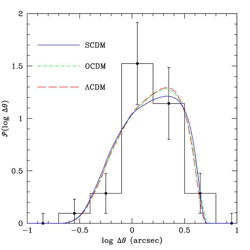
As suggested by Keeton (1998), a plausible way to reconcile simple statistical lensing models with the data on image separations of QSOs is to consider the dissipation and cooling of the baryonic protogalactic component and the radial re-distribution of the collisionless dark matter as a consequence of baryonic infall (e.g. Blumenthal et al. 1986). The net effect is a compression which transforms galaxy sized NFW halos into nearly isothermal distributions. Group and cluster halos instead maintain their NFW profile, and are extremely inefficient lenses compared to the corresponding SIS. Since baryonic cooling is effective in halos having masses smaller than a threshold value roughly independent of (Rees & Ostriker 1977; Silk 1977), the picture adopted in this paper comprises then a collection of isothermal spheres for and a set of NFW halos for . We have selected the value of empirically, by using the Kolmogorov-Smirnov test to optimize the agreement with the data on angular separations available in the CASTLE (CfA-Arizona-Space-Telescope-LEns) survey. As shown in Figure 1, a ‘transition’ mass of provides a best-fit value for all the relevant cosmologies. As multiply imaged systems with large angular separations are always produced by massive NFW halos, a reduction (with respect to the PS+SIS case discussed in the previous section) of the expected fraction of large separation systems to levels compatible with observations is obtained.
2.4 Lensing optical depth in CDM cosmologies
We analyze the frequency of lensing events in three different cosmologies with parameters suggested by a variety of recent observations: an open model (OCDM, , ), a flat model (CDM, , ), and an Einstein-de Sitter model (SCDM, , ). In all cases the amplitude of the power spectrum or, equivalently, the value of the rms mass fluctuation in a Mpc sphere, , has been fixed in order to reproduce the observed abundance of rich galaxy clusters in the local universe (e.g. Eke, Cole & Frenk 1996; Jenkins et al. 1998).333Here and below we denote the present-day Hubble constant as . The model parameters are shown in Table 1. The “cosmic concordance” model proposed by Ostriker & Steinhardt (1995) has been selected to represent the whole class of -dominated cosmogonies (CDM). While this model is able to account for most known observational constraints, ranging from globular clusters ages through CMB anisotropies to recent analyses of the Type Ia SNe Hubble diagram, it may be in marginal conflict with the statistics of gravitational lenses (Kochanek 1996). Our choice of an open CDM (OCDM) cosmology is guided by the growing evidence in favour of a low value of from cluster studies (White & Fabian 1995; Carlberg, Yee, & Ellingson 1997). For reference, and as instructive counterpart to the previous variants, we also consider a standard CDM (SCDM) scenario.
| Model | |||||
|---|---|---|---|---|---|
| SCDM | |||||
| OCDM | |||||
| CDM |
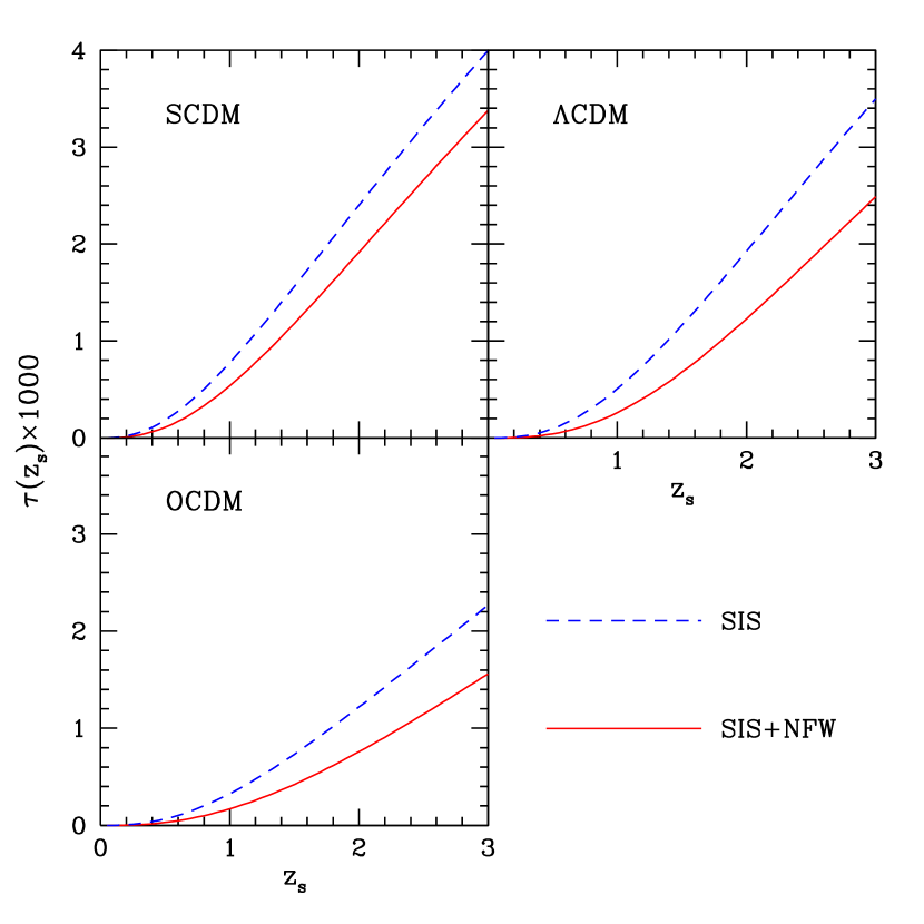
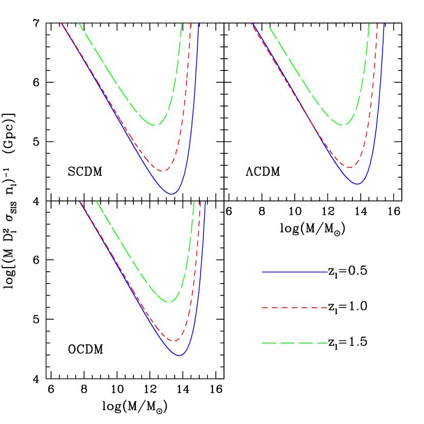
Figure 2 shows the strong lensing optical depth ( for and otherwise) for a source at redshift (also shown, for comparison, are the results obtained by assuming that every halo relaxes to a SIS). The lensing frequency is the highest in SCDM and the lowest (by about a factor of 2 at ) in OCDM cosmologies, with CDM models in between. In all cases is dominated by the contribution of SIS lenses. The relative amplitudes between different cosmological models depend on a combination of effects: (a) The geometry of the lens system affects the optical depth through the ratio and only halos in a narrow redshift interval can be efficient lenses for a source at redshift . If (), for example, the maximum contribution to comes from halos at (). For and (say), the ratios between the geometric factors in the various cosmologies are and . (b) The path-length to a source at is (in units of the Hubble radius) , , and in CDM, OCDM, and SCDM universes, respectively. (c) For a fixed mass, the halo velocity dispersion shows only a weak dependence on the world model. At , for example, in CDM is smaller than in SCDM by . On the other hand, OCDM shows the largest velocity dispersions, with larger than in SCDM by . (d) The number density of halos obviously influences the lensing frequency. Roughly speaking, for objects with mass , where is such that , the number of halos contained in a Hubble volume is proportional to , i.e. there are approximately three times more lenses in SCDM than in low-density universes. By contrast, halos with form earlier in low-density cosmogonies. In SCDM, the formation of the massive (and exponentially rare) objects which are responsible for large separation multiple images is delayed to such low redshifts that they fail to be efficient lenses for sources at . This is graphically shown in Figure 3, where the function , the mean-free-path per logarithmic mass interval of a beam to encountering a lensing event, is plotted as a function of mass for different values of and a source at . While in the SIS approximation the lensing optical depth is dominated by masses in the range to , i.e. by massive galaxies, groups, and poor clusters, a sharp drop in the mean free path is obviously present for in the combined SISNFW case. The most efficient foreground lenses are at a redshift less than unity. The larger number of lenses in SCDM more than compensate for the longer path lengths to a given redshift and earlier collapse times that characterize open and models.
It is fair at this stage to point out that, while it has become customary to model (as we have done) virialized dark matter halos by smooth distributions, observational data have recently shown the importance of considering the presence of baryonic and dark substructure in groups and clusters of galaxies (e.g. Williams, Navarro & Bartelmann 1999; Keeton 1998). The relevance for lensing of substructure and, in particular, of massive central galaxies appears to be more cospicuous in smaller aggregates. This helps explaining why all the confirmed lens systems detected so far are always produced either by galaxies (multiply imaged quasars and radio sources) or by the halos of large clusters (arc systems). Those lens systems which are clearly associated with a group or a small cluster are always dominated by the lensing effect of a bright galaxy rather than the dark halo of the group. While a detailed analysis of the effect of substructures is clearly beyond the scope of this paper, we expect that our predictions for groups and small clusters may tend to underestimate their lensing optical depth (see also Williams et al. 1999).
It is also worth stressing that the PS mass function has been recently shown to overpredict the number density of halos in the low-mass tail of the distribution by a factor 1.5–2 with respect to high-resolution –body simulations (e.g. Gross et al. 1998). In order to test how this inaccuracy of the PS formula affects the computation of the strong lensing optical depth, we have re-calculated according to equation (1) after replacing the PS mass function with the formula derived by Sheth & Tormen (1999) in order to reproduce the –body outcome. We find that, given the overall degree of uncertainty of our calculations, the inaccuracy of the mass function does not represent a major issue. For example, in the SCDM model and for , the strong lensing optical depth derived from –body simulations is smaller than its PS counterpart by only 20%.
Another simplifying assumption we have made involves the spatial distribution of the lens population, here modeled with a Poisson process. Indeed, the clustering properties of dark halos are known to slightly alter the lensing statistics. In particular, the presence of rich aggregates and large voids will increase the frequency of events in the low- and high-magnification tails of the distribution (e.g. Jaroszyński 1992).
2.5 Galaxy lensing
As a way to gauge the possible shortcomings of the PS method discussed above [e.g. the intrinsic lack of accuracy at the low-mass tail as well as uncertainties in or in the conversion between mass and velocity dispersion or concentration], it is interesting to consider in some detail the contribution of known galaxies to the magnification frequency. We model the lensing galaxies again as SIS. Their luminosity function,
| (12) |
includes just early E/S0 types, as late spirals and irregulars are known to make a small contribution () to the lensing statistics (Kochanek 1996; Maoz & Rix 1993). The velocity dispersion of the dark matter in each galaxy halo is related to the luminosity through a Faber-Jackson law
| (13) |
The assumption that the local properties of E/S0 galaxies persist out to has some observational basis (e.g. Lilly et al. 1995; van Dokkum et al. 1998). It also appears that, by and large, the statistics of multiply imaged QSOs is consistent with the locally observed galaxy population extrapolated to higher redshifts (Kochanek 1993; Maoz & Rix 1993). If the galaxy comoving number density does not change with cosmic time, and one neglects all evolutionary corrections to equation (13), equation (1) can be simplified, and the lensing optical depth becomes proportional to a dimensionless constant factor (Turner, Ostriker, & Gott 1984)
| (14) |
where is Euler’s gamma function. We use the best-fit ES0 Schechter parameters from the SSRS2 samples (, Marzke et al. 1998): , , and (the absolute blue magnitude associated with a luminosity ). With a fiducial value of (Kochanek 1994), this model yields (cf. Fukugita & Turner 1991). For comparison, the all-type luminosity function from the Autofib survey (, Ellis et al. 1996), when scaled by the Postman & Geller (1984) fraction (31%) of E/S0 galaxies, gives , , , and . With these assumptions, cosmology only affects the lensing optical depth through geometric effects, and the number of lensed sources is the highest in a CDM model. How does the optical depth for strong galaxy lensing compare then with the PS+SIS+NFW frequency shown in Figure 2? For a source at (say) , the former (with Ellis et al. parameters) is 1.3 times larger than the latter in OCDM, 1.4 times larger in CDM, and 2.9 times smaller in SCDM. The number of galaxy lenses is two times smaller with Marzke et al. parameters. In order to include the effects of galaxy groups and clusters, in the following sections we shall estimate the number of magnified SNe from the PS formalism in a SCDM cosmology. It is clear from the above discussion, however, that the uncertainties in the lensing optical depth are non-negligible. One should also keep in mind that the PS mass function, with , is significantly steeper at the low-mass end than that derived from equations (12), and (13), . Barring selection effects, the statistics of gravitational lensing within the PS theory will tend to overestimate the frequency of small-separation images.
3 Supernovae
3.1 Rates
The rates of SNe as a function of cosmic time depend on the star formation history of the universe, , the initial mass function (IMF) of stars, , and the nature of the binary companion in Type Ia events. The frequency of core-collapse supernovae, SN II and possibly SN Ib/c, which have short-lived ( Myr) progenitors (e.g. Wheeler & Swartz 1993), is essentially proportional to the instantaneous stellar birthrate of stars with mass . For a Salpeter IMF (with lower and upper mass cutoffs of 0.1 and 125 ), the core-collapse supernova rate can be related to the star formation rate per unit comoving volume according to
| (15) |
By contrast, the specific evolutionary history leading to a Type Ia event is poorly known. SN Ia are believed to result from the explosion of C-O white dwarfs (WDs) triggered by the accretion of material from a companion, possibly another WD or a non-degenerate, evolved star (e.g. Ruiz-Lapuente, Canal, & Burkert 1997). The clock for the explosion is set by the lifetime of the primary star and, e.g., by the time taken for a non-degenerate companion to evolve and fill its Roche lobe (or, in the case the companion is another WD, the orbital decay time following gravitational wave emission). The evolution of the rate may depend then, among other things, on the unknown mass distribution of the secondary binary components and on the distribution of initial orbital separations. In this sense Type Ia SNe follow a slower evolutionary clock than Type II’s, and their rate at any given time is sensitive to the past history of star formation in galaxies. Here we follow Madau, Della Valle, & Panagia (1998, hereafter MDP), and parameterize the rate of Type Ia’s in terms of a characteristic explosion timescale, (which defines an explosion probability per WD assumed to be independent of time), and an explosion efficiency, . The former accounts for the time elapsed in the various scenarios from a newly born (primary) WD to the SN explosion itself, the latter for the fraction of stars in binary systems that will never undergo a SN Ia explosion because of unfavorable initial conditions. The rate of Type Ia events at any one time is then given by the explosions of all the binary WDs produced in the past that have not gone off already, i.e.
| (16) |
where , is the minimum mass of a star that reaches the WD phase at time , and is the standard lifetime of a star of mass (all stellar masses are expressed in solar units).
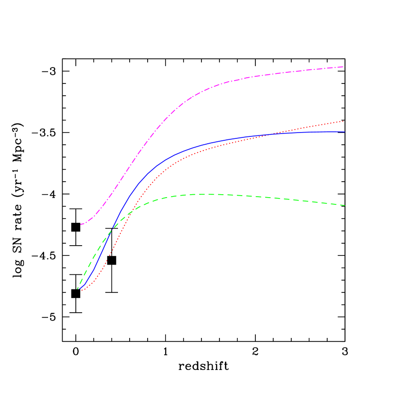
Figure 4 shows the predicted Type Ia and II rates per unit proper time and unit comoving volume for a cosmic star formation history that traces the rise from to of the galaxy UV emissivity (Madau, Pozzetti, & Dickinson 1998). The stellar evolution model (depicted in Figure 1b of MDP) assumes a Salpeter IMF and a weakly increasing star formation density above , and is able to account for the entire optical background light recorded in the galaxy counts: half of the present-day stars – the fraction contained in spheroidal systems – formed at . Because of the uncertainties in the amount of starlight that is absorbed by dust and re-radiated in the far-IR as a function of cosmic time, these numbers are only meant to be indicative. Our estimates may be on the conservative side, as the assumed stellar evolution model produces only a fraction of the IR background detected by COBE (Dwek et al. 1998). On the other hand, dust along the line-of-sight may affect the detectability of Type II SNe (and also Type Ia’s if the explosion delay timescale is short enough that dust is retained in the star-forming regions.) No attempt has been made to include the possibility of optically hidden SNe in our calculations.
The Type Ia rates plotted in the figure assume characteristic “delay” timescales after the collapse of the primary star to a WD equal to and 3 Gyr, which virtually encompass most relevant possibilities. For a fixed initial mass , the frequency of Type Ia events peaks at an epoch that reflect an “effective” delay from stellar birth. A prompter (smaller ) explosion results in a higher SN Ia rate at early epochs. The explosion efficiency () was adjusted to reproduce the observed ratio of Type II to Type Ia rates in the local universe. When normalized to the emitted blue luminosity density, the predicted frequencies match rather well the data at (MDP).
3.2 Number counts of SN Ia
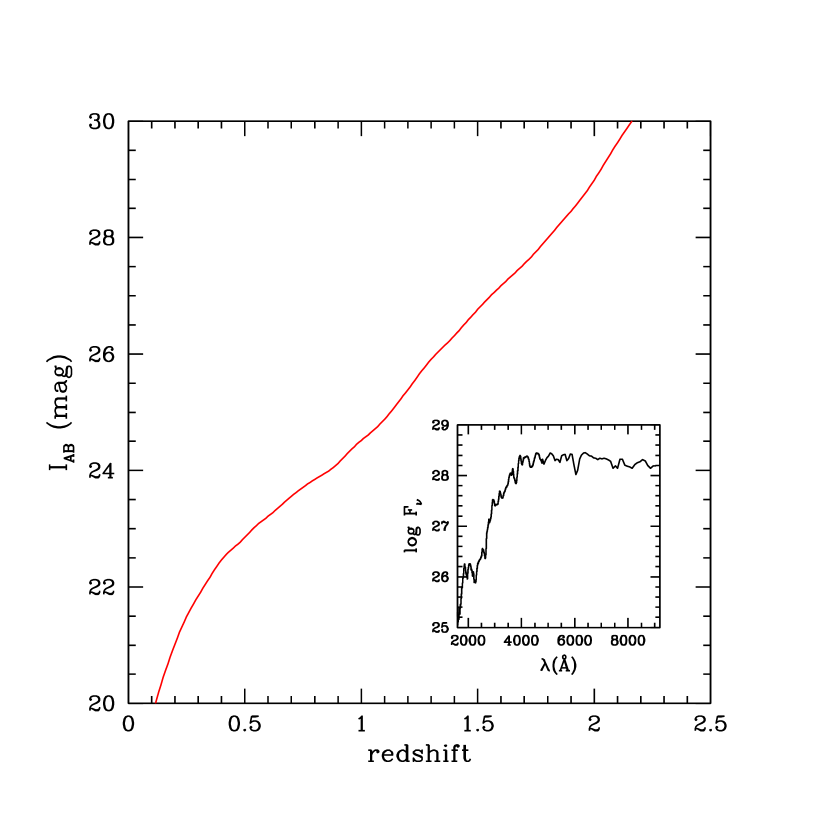
In this section we will derive the observationally relevant quantity, i.e. the rate of significantly magnified SNe in a flux-limited survey, given a cosmological model, lens population, and star formation history. An apparent magnitude-redshift relation for unlensed SNe is needed to estimate the number counts of distant Type Ia events. Traditional (i.e. from observed - to emitted -band light) -corrections out to have been calculated by Hamuy et al. (1993) using available spectra of nearby SN Ia. Multi-band photometry has been used to extend these results out to (Kim, Goobar & Perlmutter 1996). No accurate -corrections have been determined, however, for supernovae at , as very few ultraviolet spectra from the local samples with good signal-to-noise ratio are currently available. To circumvent this problem we have constructed an (unlensed) magnitude-redshift relation for Type Ia’s by using as a template the –FOS spectrum of SN 1992A taken 5 days after maximum blue light (Kirshner et al. 1993). No correction for foreground and intrinsic extinction is apparently needed for this event (Burnstein & Heiles 1984; Kirshner et al. 1993). The observed spectrum has been renormalized to a brightness (at maximum -light) of . The relation in the -band is shown in Figure 5 for . Note that, because of the steep optical/UV spectrum of 1992A, our template Type Ia SN at will be much brighter in the near-IR () than in the optical (). The -correction significantly weakens the observed flux relative to the luminosity distance effect.
For the intrinsic luminosity function of SN Ia, , we have adopted a Gaussian distribution with standard deviation mag (cf. Van den Bergh & McClure 1994). The luminosity function of lensed sources, , can be obtained by convolving with the magnification probability density (Vietri & Ostriker 1983)
| (17) |
where is the probability of having magnification for a source at redshfit , normalized so that . The observed rate on the sky of Type Ia events is then
| (18) |
where is the comoving volume element surveyed, and the factor accounts for the cosmological time dilation.444Note that, as in a snapshot survey SNe are not necessarily detected at maximum light, the total number of events will actually depend on the effective timescale over which a SN can be observed above threshold. From equation (17) we find
| (19) |
where is the minimum magnification needed to detect a source in a flux-limited survey. The above equation relates the number counts to the probability distribution of magnification discussed in § 2 for SIS lenses. In the case of NFW halos, we first solve the lens equation for a set of values of and of the dimensionless impact parameter . The magnitudes of the resulting images and the values of the corresponding impact parameters are stored in a file. The optical depth for a given magnification and source redshift is then computed using equation (1): the suitable cross sections are calculated by interpolating over the list of solutions of the lens equation, and by using the method described in the appendix of NFW to evaluate the scale radius of a selected halo.
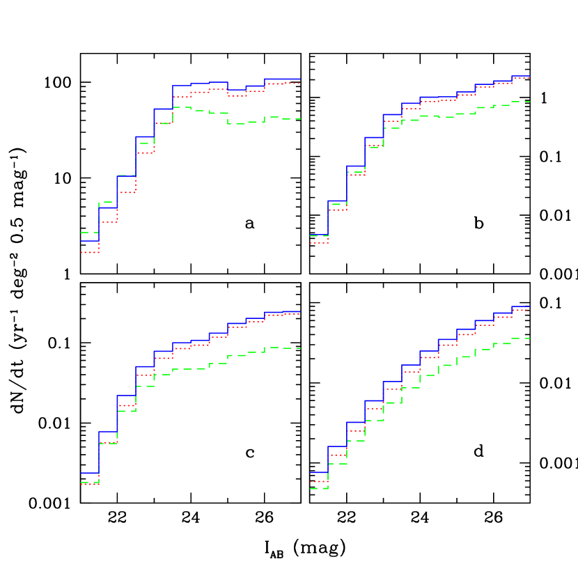
To compute the total number of supernovae brighter than that have been gravitationally magnified by more than magnitudes, the function in equation (19) must be integrated from to infinity. Our treatment will be limited to magnifications mag, i.e. to images that are more than 2 away from the mean intrinsic luminosity of SN Ia. In this regime, the weak (with typical magnifications of the order of a few per cent) lensing due to large scale structure can safely be neglected. Figure 6 shows the counts of SNe Ia at maximum -light for a SCDM cosmology. The rate of detection in the absence of gravitational lensing effects (which is very close to the total expected number of events, since the probability of lensing is small) is compared with the estimated rates of multiply-imaged events (obtained by requiring that at least two images are sufficiently bright to enter the flux-limited sample; e.g., for SIS lenses, using eq. 6), and with the rates of individual SNe magnified by more than 0.3 and 0.75 magnitudes (for strongly lensed SNe, only the brightest image is considered; i.e., for SIS lenses, is computed using the cross section in eq. 5, while, for NFW halos, the above mentioned numerical scheme is adopted). Note that, for low magnifications (), the lensing cross section of NFW halos is comparable (and generally larger) than that of the corresponding SIS halos. Only considering multiply imaged systems, the relation holds.
In a one square degree field, and for an effective observation duration of 1 yr, the total expected number of Type Ia SNe down to mag is (assuming Gyr) . About 3.7 events will be gravitationally lensed by more than 0.3 mag, 0.5 by more than 0.75 mag, and only 0.1 will have detectable double images. These numbers are sensitive to the assumed explosion timescale. Given a well-determined cosmic star formation history, it may be possible to infer something about the nature of Type Ia SNe from the observed number counts. It is also interesting to note that, in general, gravitational magnification facilitates the detection of SNe at higher redshift in a flux-limited sample, and the fraction of lensed SNe tends to be higher at fainter magnitudes if the rate of events increases with look-back time and the gain in available volume is not balanced by a large -correction. For , this is true up to . For fainter magnitudes, the increase in physical volume is smaller and the SN rate saturates (cf. Fig. 4); deeper searches will not lead then to an increased fraction of magnified sources. This defines an optimal survey sensitivity in the -band for Type Ia’s magnified by mag of (cf. Linder et al. 1988). By contrast, there is no optimal flux threshold for detecting double images (Fig. 6d) in succession.
3.3 Number counts of SNe II
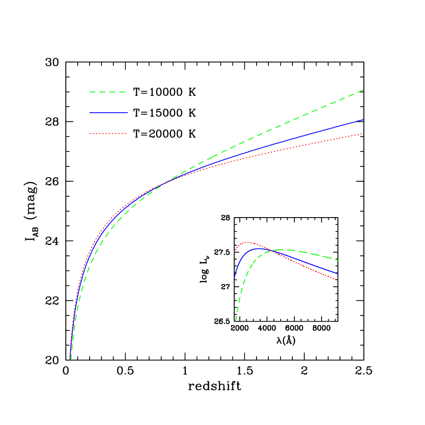
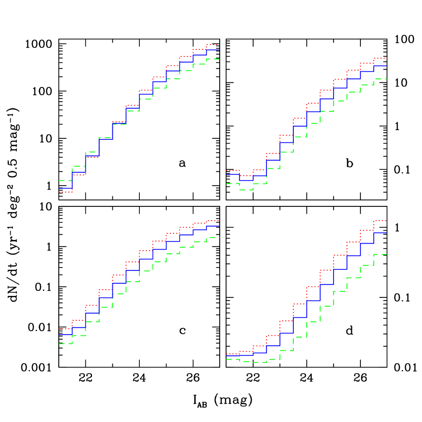
Type II SNe are a couple of magnitudes fainter than SN Ia in the rest-frame blue band. Contrary to Type Ia’s, they have a very wide luminosity function, which is well represented by a broad Gaussian distribution with (max) and dispersion 1.2 mag (Tammann & Schröder 1990).555For the present purposes, we shall ignore the possibility of an extended tail of Type II events at bright (Patat et al. 1994) and faint (Woltjer 1997) magnitudes. The spectra of most SN II at maximum light approximate well a single-temperature Planck function of about 15000 K from the UV through IR – by contrast, Type Ia’s exhibit a prominent UV deficit relative to the blackbody fit at optical wavelengths (e.g. Filippenko 1997). The difference in behavior of the -correction is clearly visible in Figure 7, where the -band relation for Type II’s is plotted for three different photospheric temperatures at peak. In the absence of dust reddening, the intrinsically fainter SN II appear brighter than SN Ia already at . This has a strong effect on the expected number counts, shown in Figure 8. At mag, there is one SN II every 2.3 Type Ia’s. The detection rate increases to one Type II every 1.2 SN Ia at , and to one every 0.56 at . Because of the flat -correction and wide luminosity function, the fraction of lensed events is higher for Type II’s, as only small magnifications are needed to bring high redshift events above the flux threshold (see also Linder et al. 1988).
3.4 Multiple images and time delays
Although exceedingly rare in the field, multiply imaged Type Ia SNe are of particular interest for cosmography, as the propagation time from the source to the observer varies from one image to another, and can be accurately measured if the source has a well defined light curve. The time delay is proportional to the absolute scale of the lens geometry and hence inversely proportional to the Hubble constant (Refsdal 1964). Given a reliable time delay measurement, a well-constrained lensing mass distribution (with a measured redshift and velocity dispersion), and a world model, one could estimate .
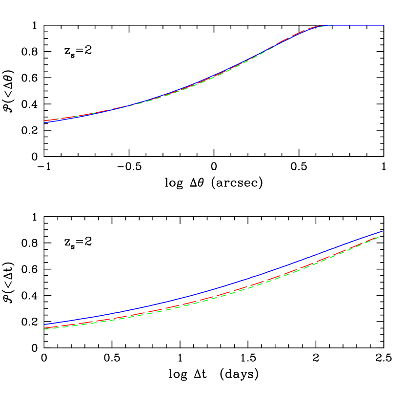
The cumulative probability functions of image separations and time delays for a SN at in the field are shown in Figure (9). About 60% (SCDM) of double images will have angular separations , and will therefore be flagged as multiple events in ground-based surveys only if the time delay is comparable or larger than the SN decay time. The fraction of images with is of order 1.5%. Barring selection effects (see below), approximately 25% of mirror events will be observed with an arrival time difference of days, 40% with days, 50% with days. The frequency distributions have been computed by modifying equation (1) to account for that fact that, at any redshift, only halos having mass larger than a threshold value can generate two images with a given angular separation or time delay. Normalizing the total probability to unity, and considering only SIS halos with (whose contribution dominates the strong lensing optical depth), one gets
| (20) |
where is the mass that, for given and , produces a separation [equal to for a SIS]. Similarly, one obtains
| (21) |
where is the time delay at and solves . Note that, because of the small strong lensing cross section of NFW halos, the presence of very large dark matter halos in OCDM and CDM universes does not create an extended tail towards large separations and long delays.
3.5 Selection effects
A peculiar feature of SNe Ia relative to QSOs is the relatively short lifetime of their emission. While, for example, the finite angular resolution of the observations may not allow to distinguish multiple images with separation on the sky , if the time delay between different images is comparable or longer than the typical decay time of a SN light curve [ days], two mirror copies will appear roughly in the same position of the sky but at different times. In this sense, even two images with could in practice flag a strong lensing event if : the same SN would go off in two (or more) incarnations of the same explosion, and the different images will be seen in succession. Because of the geometry of the source-lens-observer system, longer time delays will be obtained when the deflector is closer (in redshift) to the radiation source. Consider, e.g, a SN at in a SCDM cosmology, lensed by a massive SIS halo (, ) at . Two images will result, with (say). For a source-lens alignment , the magnifications of the images will be and , and the arrival time difference days. Unresolved images with shorter delays may still be recognizable due to the large discrepancy between the apparent expected magnitude and the one observed, and a characteristic doubly-humped light curve. At fixed and , the angular separation between the lensed images depends only on the mass of the deflector, while the time delay is anti-correlated with the magnification: smaller delays correspond to more perfect source-lens alignments and thus to larger magnifications. Nearly synchronous images will then have rather similar brightnesses. A SN at , lensed by a SIS halo at with mass (, SCDM), will produce when two well resolved images (), with magnifications and . The arrival time difference is only 20 days in this example. For SIS lenses, the maximum time delay occurs when (), hence less massive deflectors will always produce small-separation events and relatively short delays.
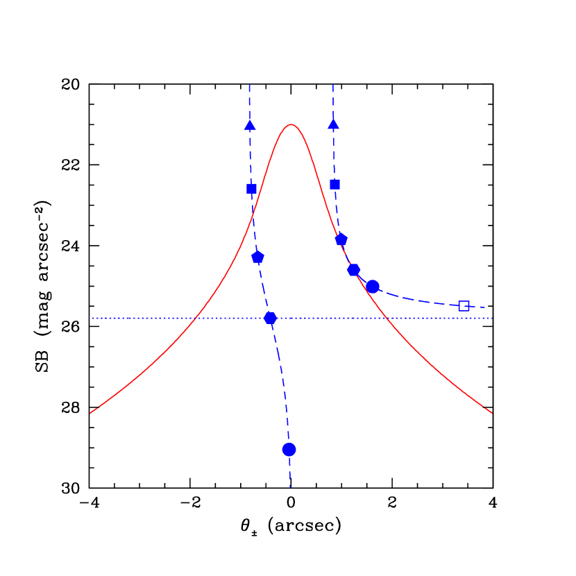
A serious bias against the detection of small-separation images is due to the luminosity of the lensing galaxy. Galaxy-type halos with velocity dispersion completely dominate the rate of small-separation events. These must then be detected in the background of a lens elliptical galaxy, most probably at . Figure 10 compares the observed surface brightness of a foreground elliptical with a background lensed Type Ia SN as a function of angular distance from the galaxy center. The effect of atmospheric seeing has been approximated by convolving the true source flux with a Gaussian of dispersion . Even in the case of excellent FWHM seeing, the lens will greatly outshine the faintest SN image. Double events will only be detectable for nearly perfect lens-source alignments, an extremely rare case. In more modest seeing conditions (FWHM), even the brightest image may remain undetected. From the ground, multiple SN events will be more easily observed in the background of a galaxy group or cluster.
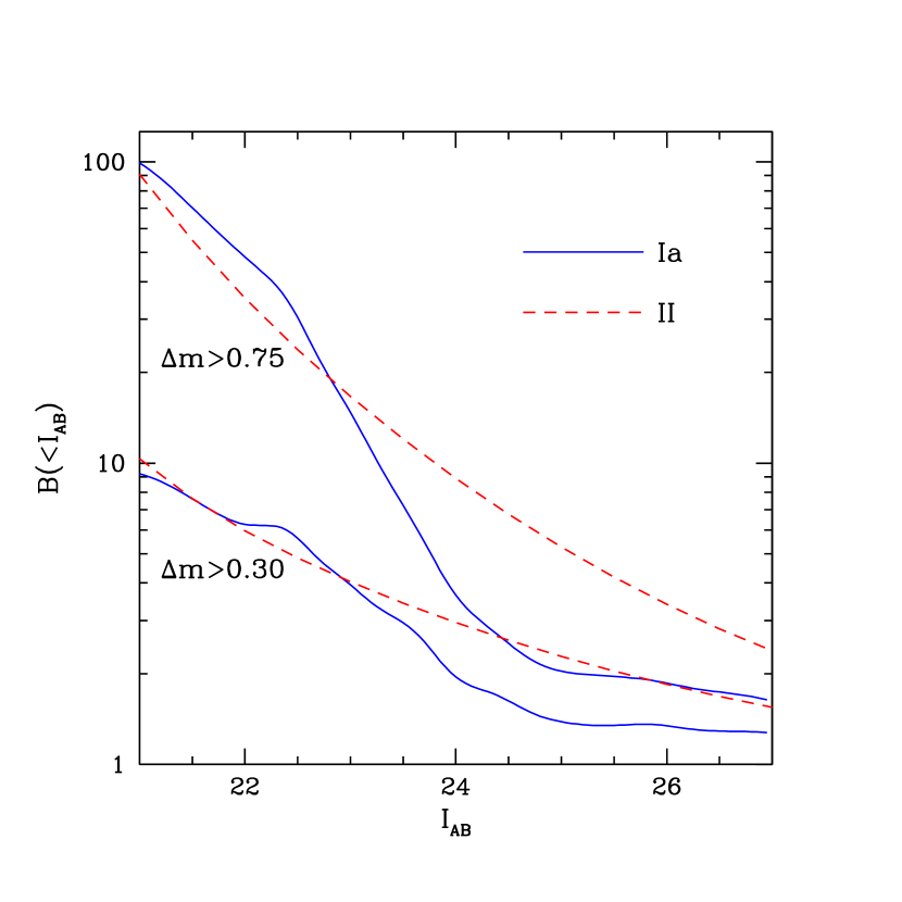
In a magnitude-limited sample, the sources that are observed to be gravitationally lensed include not only the lensed objects that are intrinsically brighter than the flux limit, but also sources that are intrinsically fainter and are brought into the sample by the magnification. Relative to the lensing optical depths shown in Figure 2, lensed systems will then be overrepresented among SNe of a given apparent magnitude. We have quantified this effect from the Type Ia and Type II number counts, by defining the magnification bias as the ratio between the actual flux-limited counts of sources magnified by more than and the counts of lensed SNe that are intrinsically brighter than the flux limit,
| (22) |
where . This definition generalizes that given in Turner, Ostriker, & Gott (1984) and Fukugita & Turner (1991) by taking into account the redshift dependence of the lensing optical depth.666In the notation of Fukugita & Turner, our approach is equivalent to a flux-dependent lensing optical depth, as fainter objects are typically at higher redshifts than bright ones. The magnification bias corresponding to and 0.75 mag is plotted in Figure 11 for Type Ia ( Gyr) and Type II SNe ( K). At the effect is huge, as the apparent frequency of events with is boosted by a factor of . Note that at these magnitude levels the counts are still nearly Euclidean: the large bias is actually due to the rapidly increasing lensing frequency with lookback time. In the standard treatment with non-evolving optical depth, a large magnification bias is typically associated with integral number counts that increase faster than , where is the observed flux (e.g. Schneider, Ehlers & Falco 1992).
3.6 Microlensing
A modulation of the SN light curve may take place if, on top of the galaxy, group, or cluster magnification, a microlensing event occurs due to individual stars or MACHOs in the galaxy halo or intracluster medium. The timescale for microlensing-induced variations is determined by two competing effects: the expansion velocity of the SN photosphere and the relative transverse motion between the microlens and the light bundle. The radius of a SN at maximum light is cm, corresponding to an observed angular dimension of . A compact object along the line-of-sight to the SN will give rise to a detectable time dependent amplification only when (Schneider & Wagoner 1987), where is the angular impact parameter. Modeling the deflector with a Schwarzschild lens of mass (i.e. neglecting the shear induced by the gravitational field of the host halo), the first condition gives
| (23) |
Less massive MACHOs can efficiently magnify the SN only during its fast light-rising time. For , the duration of the microlensing event roughly corresponds to the time needed by the photosphere to fill the Einstein ring of the lens (see also Gould 1994). For a typical photospheric expansion velocity of , one obtains
| (24) |
This is usually much shorter than the characteristic crossing time of the Einstein ring
| (25) |
where is the relative transverse velocity between microlens and source. In a SCDM cosmology with and , one finds and . The microlensing timescale is then comparable with days (SN Ia) for very small microlens masses. Only MACHOs with can then produce detectable ‘noise’ that will degrade the light curves of the macroimages. More massive objects will boost the magnification of the SN image for the entire duration of the macroevent.
4 Summary
All previous studies of the influence that a population of deflectors has on the observational properties of background objects have considered sources like galaxies or quasars that are quite inhomogeneous, i.e. have a wide range of intrinsic luminosities, ellipticities, etc. By contrast, Type Ia SNe represent a population of objects with well-known intrinsic properties, and could – in addition to their use as reliable cosmological distance indicators and valuable tracers of the star formation history in galaxies – potentially flag the occurrence of a gravitational lensing event even in the absence of multiple or highly distorted images. We have investigated the lensing effect of background SNe due to virialized dark matter halos in CDM cosmogonies, and computed lensing frequencies, rates of SN explosions, and distributions of arrival time differences and image separations. Within the assumption that dark halos approximate singular isothermal spheres on galaxy scales and NFW profiles on group/cluster scales, and are distributed in mass according to the Press-Schechter theory, about one every 12 Type Ia SNe at will be magnified by (SCDM). Using recent estimates of the global history of star formation to compute the expected frequencies of SNe as a function of cosmic time, we have derived a detection rate of Type Ia’s with magnification mag of a few events yr-1 deg-2 at maximum -light and . Events with mag are 7 times less frequent. Only about one fifth of them give rise to observable multiple images: the SN will appear as multiple events with identical light curves, separated in time and differing only by the scaling of their amplitudes. Because of the flat -correction and wide luminosity function, we find that Type II SNe will dominate the number counts at and have the largest fraction of lensed objects. At bright magnitudes, the effect of magnification bias on the apparent frequency of lensed SNe with is huge, a factor of in samples with . The enhancement of the lensing probability beyond the optical depth expectation drops to a factor of 3.5 at 24 mag (26 mag) in the case of Type Ia SNe (SN II). The apparent magnitude of the lens galaxy introduces a serious selection effect, as it reduces the detectability of small-separation multiple events in ground-based searches.
On the face of their rarity, it is not unconceivable that large consortia of new and existing SN search teams may conduct in the near future deep pencil beam surveys and be able to detect magnified Type Ia’s up to (Wang 1998). Current searches have been limited so far to mag. A second-epoch deep ( mag) observation of the Hubble Deep Field by Gilliland, Nugent, & Phillips (1999) has recently revealed a Type Ia SN. The combination of a new generation of large telescopes with 1 degree field of view and multi-fiber spectrometers, together with faster techniques such as the snapshot distance method (Riess et al. 1998), could soon yield more than new events per year. As suggested by Kolatt & Bartelmann (1998), one could also look for lensed SNe in the background of massive clusters. A nearby rich cluster at with virial mass of and NFW profile will magnify by more than mag every point source lying at less than from its center. The expected rate of SNe Ia behind such a cluster with a mismatch of mag is then events per year with (SCDM, Gyr). Along the same lines, Kovner & Paczynski (1988) have proposed the possible identification of Type II SNe in the lensed giant arcs observed in the cores of clusters of galaxies. If a SN goes off within the caustic and close to the cusp of the cluster potential, it will be detected as three (or more) spatially-separated events with time delays as short as a few weeks or even days. The blue color of the arcs suggests significant star formation hence a high rate of SN explosions. Incidentally, if the cluster potential were understood well enough that a reasonable estimate of the time delay was available, one could exploit the occurrence of delayed mirror events to study such transient phenomena in much greater details that would be possible without prior warning.
Looking further into the future, it is interesting to consider the detectability of lensed Type Ia and Type II SNe with the Next Generation Space Telescope (NGST). A typical SN II at would give rise to an observed flux of 8 nJy (SCDM) at 2.6 µm. At this wavelength, the imaging sensitivity of an 8m NGST is around 1.5 nJy ( s exposure and detection threshold), while the moderate resolution () spectroscopic limit is about 50 times higher ( s exposure per resolution element and detection threshold, Stockman et al. 1998). Depending on the history of star formation at high redshifts, the NGST could detect Type II SNe (at peak brightness) per field per year at (MDP; cf. Dahlén & Fransson 1999; Miralda-Escudé & Rees 1997). (In principle, Type Ia’s could also be imaged at extreme redshifts, , but the long delay times from stellar birth characteristic of these events make a detection rather improbable.) We find that, even for sources at these early epochs, the optical depth for strong lensing is small, for and SCDM. Marri & Ferrara (1998) have recently explored in details the observational perspectives for Pop III SNe detection with the NGST when gravitational magnification is taken into account. They computed lensing frequencies and magnification maps using a ray-shooting numerical technique and assuming point-like lenses. Our more realistic treatment implies probabilities that are much lower than theirs, as isothermal spheres and NFW halos are very inefficient magnifiers compared to point-like deflectors of the same mass.
Acknowledgements.
We have benefited from useful discussions with B. Bassett, R. Blandford, C. Keeton, N. Panagia, and P. Schneider. We thank R. Kirshner for providing us with the HST–FOS spectrum of SN 1992A, and the referee, C. Kochanek, for many comments that vastly improved the manuscript. Support for this work was provided by NASA through ATP grant NAG5-4236.References
- (1) Babul, A., & Lee, M. H. 1991, MNRAS, 250, 407
- (2) Bartelmann, M. 1996, A&A, 313, 697
- (3) Blandford, R. D., & Narayan, R. 1992, ARA&A, 30, 311
- (4) Blandford, R. D., Saust, A. B., Brainerd, T. G., & Villumsen, J. V. 1991, MNRAS, 251, 600
- (5) Blumenthal, G. R., Faber, S. M., Flores, R., & Primack, J. R. 1986, ApJ, 301, 27
- (6) Burnstein, D., & Heiles, C. 1984, ApJS, 54, 33
- (7) Cappellaro, E., Turatto, M., Tsvetkov, D. Yu., Bartunov, O. S., Pollas, C., Evans, R., & Hamuy, M. 1997, A&A, 322, 431
- (8) Carlberg, R. G., Yee, H. K. C., & Ellingson, E. 1997, ApJ, 478, 462
- (9) Dahlén, T., & Fransson, C. 1999, A&A, in press (astro-ph/9905201)
- (10) Dwek, E., et al. 1998, ApJ, 508, 106
- (11) Dyer, C. C., & Roeder, R. C. 1973, ApJ, 180, L31
- (12) Ehlers, J., & Schneider P. 1986, A&A, 168, 57
- (13) Eke, V. R., Cole, S., & Frenk, C. S. 1996, MNRAS, 282, 263
- (14) Ellis, G. F. R., Bassett, B. A., & Dunsby, P. K. 1998, Class. Quant. Grav, 15, 2345
- (15) Ellis, R. S., Colless, M., Broadhurst, T., Heyl, J., & Glazebrook, K. 1996, MNRAS, 280, 235
- (16) Evans, R., van den Bergh, S., & McClure, R.D. 1989, ApJ, 345, 752
- (17) Falco, E. E., Gorenstein, M. V., & Shapiro, I. I. 1991, ApJ, 372, 364
- (18) Filippenko, A. V. 1997, ARA&A, 35, 309
- (19) Flores, R., & Primack, J. R. 1996, ApJ, 497, L5
- (20) Frieman, J. A. 1996, Comments Astrophys., 18, 323
- (21) Fukugita, M., & Turner, E. L. 1991, MNRAS, 253, 99
- (22) Fukugita, M., Futamase, T., Kasai, M., & Turner, E. L. 1992, ApJ, 393, 3
- (23) Garnavich, P. M., et al. 1998, ApJ, 493, L53
- (24) Gilliland, R. L., Nugent, P. E., & Phillips, M. M. 1999, ApJ, 521, 30
- (25) Gould, A. 1994, ApJ, 421, L71
- (26) Grogin, N. A., & Narayan, R. 1996, ApJ, 473, 570
- (27) Gross, M. A. K., Somerville, R. S., Primack, J. R., Holtzman, J., & Klypin, A. 1998, MNRAS, 301, 81
- (28) Hamuy, M., Phillips, M. M., Suntzeff, N. B., Schommer, R. A., Maza, J., & Aviles, R. 1996, AJ, 112, 2391
- (29) Hamuy, M., Phillips, M. M., Wells, L. A., & Maza, J. 1993, PASP, 105, 787
- (30) Holz, D. E. 1998, ApJ, 506, L1
- (31) Jaroszyński, M. 1992, MNRAS, 255, 655
- (32) Jenkins, A., et al. 1998, ApJ, 499, 20
- (33) Kaiser, N. 1992, ApJ, 388, 272
- (34) Kantowski, R., Vaughan. T., & Branch, D. 1995, ApJ, 447, 35
- (35) Keeton, C. R. 1998, PhD thesis, Harvard University
- (36) Kim, A., Goobar, A., & Perlmutter, S. 1996, PASP, 108, 190
- (37) Kirshner, R. P., et al. 1993, ApJ, 415, 589
- (38) Kochanek, C. S. 1993, ApJ, 419, 12
- (39) Kochanek, C. S. 1994, ApJ, 436, 56
- (40) Kochanek, C. S. 1995a, ApJ, 445, 559
- (41) Kochanek, C. S. 1995b, ApJ, 453, 545
- (42) Kochanek, C. S. 1996, ApJ, 466, 638
- (43) Kochanek, C. S., Blandford, R. D., Lawrence, C. R., & Narayan, R. 1989, MNRAS, 238, 43
- (44) Kolatt, T. S., & Bartelmann M. 1998, MNRAS, 296, 763
- (45) Kovner, I., & Paczynski, B. 1988, ApJ, 335, L9
- (46) Kravtsov, A. V., Klypin A. A., Bullock J. S., & Primack, J. R. 1998, ApJ, 502, 48
- (47) Kundic, T., et al. 1997, ApJ, 482, 75
- (48) Lacey, C., & Cole S. 1993, MNRAS, 262, 627
- (49) ——– 1994, MNRAS, 271, 676
- (50) Lahav, O., Lilje, P. B., Primack, J. R., & Rees, M. J. 1991, MNRAS, 251, 128
- (51) Lilly, S. J., Tresse, L., Hammer, F., Crampton, D., & Le Févre, O. 1995, ApJ, 455, 108
- (52) Linder, E. V., Schneider, P., & Wagoner, R. V. 1988, ApJ, 324, 786
- (53) Lynds, R., & Petrosian, V. 1989, ApJ, 336, 1
- (54) Madau, P., Della Valle, M., & Panagia, N. 1998, MNRAS, 297, L17 (MDP)
- (55) Madau, P., Pozzetti, L., & Dickinson, M. E. 1998, ApJ, 498, 106
- (56) Maoz, D., & Rix, H.-W. 1993, ApJ, 416, 425
- (57) Maoz, D., Rix, H.-W., Gal-Yam, A., & Gould, A. 1997, ApJ, 486, 75
- (58) Marri, S., & Ferrara, A. 1998, ApJ, 509, 43
- (59) Marzke, R. O., da Costa, L. N., Pellegrini, P. S., Willmer, C. N. A., & Geller, M. J. 1998, ApJ, 503, 617
- (60) Metcalf, R. B. 1999, MNRAS, 305, 746
- (61) Miralda-Escudé, J., & Rees, M. J. 1997, ApJ, 478, L57
- (62) Moore, B., Quinn, T., Governato, F., Stadel, J., & Lake G. 1999, submitted to MNRAS (astro-ph/9903164)
- (63) Narayan, R., & Bartelmann, M. 1997, in Formation of Structure in the Universe, ed. A. Dekel & J. P. Ostriker (Cambridge: Cambridge University Press), 123
- (64) Narayan, R., & White, S. D. M. 1998, MNRAS, 231, 97P
- (65) Navarro, J. F., Frenk, C. S., & White, S. D. M. 1997, ApJ, 490, 493
- (66) Ostriker, J. P., & Steinhardt, P. J. 1995, Nature, 377, 600
- (67) Pain, R., et al. 1997, ApJ, 473, 356
- (68) Patat, R., Barbon, R., Cappellaro, E., & Turatto, M. 1994, A&A, 282, 731
- (69) Perlmutter, S., et al. 1998, Nature, 391, 51
- (70) Postman, M., & Geller, M. J. 1984, ApJ, 281, 95
- (71) Press, W. H., & Schechter, P. 1974, ApJ, 187, 425
- (72) Rees, M. J., & Ostriker, J. P. 1977, MNRAS, 179, 541
- (73) Refsdal, S. 1964, MNRAS, 128, 295
- (74) Riess, A. G., Nugent, P., Filippenko, A. V., Kirshner, R. P., & Perlmutter, S. 1998, ApJ, 504, 935
- (75) Riess, A. G., Press, W. H., & Kirshner, R. P. 1996, ApJ, 473, 88
- (76) Ruiz-Lapuente, P., Canal, R., & Burkert, A. 1997, in Thermonuclear Supernovae, ed. P. Ruiz-Lapuente, R. Canal, & J. Isern (Dordrecht: Kluwer), p. 205
- (77) Schneider, P., Ehlers, J., & Falco, E. E. 1992, Gravitational Lenses (Berlin: Springer-Verlag)
- (78) Schneider, P., & Wagoner, R. V. 1987, ApJ, 314, 154
- (79) Sheth, R. K., & Tormen, G. 1999, submitted to MNRAS (astro-ph/9901122)
- (80) Silk, J. 1977, ApJ, 211, 638
- (81) Stockman, H. S., Stiavelli, M., Im, M., & Mather, J. C. 1998, in ASP Conf. Ser. 133, Science with the Next Generation Space Telescope, ed. E. Smith & A. Koratkar (San Francisco: ASP), p. 24
- (82) Tammann, G. A., Löffler, W., & Schröder, A. 1994, ApJS, 92, 487
- (83) Tammann, G. A., & Schröder, A. 1990, A&A, 236, 149
- (84) Tomita, K. 1998, Prog. Theor. Phys., 100, 1
- (85) Tremaine, S., Richstone, D. O., Byun, Y.-I., Dressler, A., Faber, S. M., Grillmair, C., Kormendy, J., & Lauer, T. R. 1994, AJ, 107, 634
- (86) Turner, E. L., Ostriker, J.P., & Gott, J. R., III 1984, ApJ, 284, 1
- (87) Tyson, J. A., & Fisher, P. 1995, ApJ, 446, L55
- (88) Tyson, J. A., Kochanski, G. P., & Dell’ Antonio, I. P. 1998, ApJ, 498, L107
- (89) Van den Bergh, S., & McClure, R. D. 1994, ApJ, 425, 205
- (90) van Dokkum, P. G., Franx, M., Kelson, D. D., & Illingworth, G. D. 1998, ApJ, 504, L17
- (91) Vietri, M., & Ostriker, J. P. 1983, ApJ, 267, 488
- (92) Villumsen, J. V. 1996, MNRAS, 281, 369
- (93) Wallington S., & Narayan R. 1993, ApJ, 403, 517
- (94) Wambsganss, J., Cen, R., Xu, G., & Ostriker, J. P. 1997, ApJ, 475, L81
- (95) Wang, Y. 1998, submitted to MNRAS (astro-ph/9806185)
- (96) Wheeler, J. C., & Swartz, D. A. 1993, Space Sci. Rev., 66, 425
- (97) White, D. A., & Fabian, A. C. 1995, MNRAS, 273, 72
- (98) Williams, L. L. .R., Navarro, J. F., & Bartelmann, M., submitted to ApJ (astro-ph/9905134)
- (99) Woltjer, L. 1997, A&A, 328, L29
- (100) Zel’dovich, Ya. B. 1964, Soviet Astron. AJ, 8, 13
- (101)
- (102)
- (103)