Coherently-Dedispersed Polarimetry of Millisecond Pulsars

Abstract

We present a large sample of high-precision, coherently-dedispersed polarization profiles of millisecond pulsars (MSPs) at frequencies between 410 and 1414 MHz. These data include the first polarimetric observations of several of the pulsars, and the first low-frequency polarization profiles for others. Our observations support previous suggestions that the pulse shapes and polarimetry of MSPs are more complex than those of their slower relatives. An immediate conclusion is that polarimetry-based classification schemes proposed for young pulsars are of only limited use when applied to millisecond pulsars.

The Astrophysical Journal Supplement Series 123, 627 (1999)

1 Introduction

The polarization characteristics of a pulsar yield clues to its magnetic geometry and emission mechanism. Many pulse profiles are highly linearly polarized and have a clear position-angle swing across part or all of the period. For slow pulsars, this position-angle swing often follows the characteristic S-shaped curve of the “rotating vector model” (RVM) introduced by Radhakrishnan and Cooke (1969). In this description, the magnetic dipole axis is inclined at an angle $\alpha$ from the spin axis, and makes angle $\beta$ with the line of sight from Earth. The angle of between the line of sight and the pulsar spin axis is $\zeta=\alpha+\beta$. The position angle $\psi$ can then be written as a function of pulse phase $\phi$:

$$\tan(\psi(\phi)-\psi_{0})\,=\,\frac{\sin\alpha\sin(\phi-\phi_{0})}{\cos\alpha\sin\zeta-\sin\alpha\cos\zeta\cos(\phi-\phi_{0})}$$ (1)

where $\psi_{0}$ is a constant offset and $\phi_{0}$ is the phase of steepest position-angle swing, given by:

$$\left(\frac{d\psi}{d\phi}\right)_{\phi_{0}}\,=\,\frac{\sin\alpha}{\sin\beta}.$$ (2)

The rotating vector model, along with the observed linear and circular polarization properties of many pulse profiles, has led to the formulation of successful phenomenological classification schemes for slow pulsars based on pulse morphology and polarimetry (e.g., Rankin (1983); Lyne & Manchester (1988)).

To date, limited polarimetric studies of the faster millisecond pulsars (MSPs) have suggested that their pulse components do not fit easily into these classification schemes, and frequently have more complex polarimetric profiles than slow pulsars (Thorsett & Stinebring (1990); Navarro et al. (1997); Xilouris et al. (1998)).

In this paper we present polarization profiles for several millisecond pulsars. These profiles represent the first polarimetric observations of many of these pulsars, and for others, the first low-frequency polarization profiles. There is considerable overlap between the present set of pulsars and those studied by Xilouris et al. (1998) at 1410 MHz using the 100 m telescope at Effelsberg, Germany; our study provides a needed complement to these higher-frequency observations. Recently, Sallmen (1998) has studied several of the pulsars presented here, conducting observations at the National Radio Astronomy Observatory, Green Bank, W.V. and Effelsberg, Germany. Where applicable, we compare our results to these studies.

2 Observations

Observations were made using the 76-m telescope at the Nuffield Radio Astronomy Laboratories, Jodrell Bank, U.K., between 1997 January and 1997 July. Data were obtained at 410 MHz, 610 MHz, and 1414 MHz, with observing bandwidths of 5 MHz at 410 MHz and 610 MHz, and 10 MHz at 1414 MHz. All data were acquired with the Princeton Mark IV observing system. This instrument implements the coherent dispersion removal technique described by Hankins and Rickett (1975). A fast analog-to-digital converter samples quadrature components of the received telescope voltages in the two orthogonal circular polarization channels, $L$ and $R$, employing either 2-bit sampling across 10 MHz of bandwidth, or 4-bit sampling across 5 MHz. The data are stored on magnetic tape for off-line processing. Coherent dedispersion is performed in software, using a special-purpose parallel processor. The data stream is typically split into either two or four sub-bands during processing. The self- and cross-products $|L|^{2}$, $|R|^{2}$, Re($L^{*}R$) and Im($L^{*}R$) are formed from the dedispersed time-series in each sub-band, then folded modulo the predicted topocentric pulse period. The full set of Stokes parameters are readily formed from these products. A complete description of the instrument, along with preliminary polarimetric results, has been published elsewhere (Stairs (1998)).

Fluxes were calibrated using an injected noise signal, the strength of which was determined by comparison with a bright continuum source of known flux. The reference sources used varied between observing sessions, but were drawn from the following list: 3C48, with an assumed flux of 15.8 Jy at 1414 MHz; 3C123, with an assumed flux of 117.6 Jy at 410 MHz, 91.8 Jy at 610 MHz, and 48.4 Jy at 1414 MHz; 3C147, with an assumed flux of 22.3 Jy at 1414 MHz; and 3C353, with an assumed flux of 129.4 Jy at 410 MHz. The uncertainties in the calibration are approximately 10%. The noise calibrator was switched on and off at (typically) 3-minute intervals throughout each 30-minute observation.

The flux in the $|R|^{2}$ channel was determined using the differences in the off-pulse baseline and the strength of the noise calibrator. The spectrum of the $|L|^{2}$ channel was found to be more variable across the observing bandwidth, making a similar calculation less reliable for this channel. Instead, the $|L|^{2}$ calibration factor was calculated so that the ratio of the off-pulse baselines in $|L|^{2}$ and $|R|^{2}$ was equal to the ratio of the known total system temperatures, i.e., the receiver temperatures corrected for telescope elevation angle and sky temperature in the direction of the pulsar ($T_{\rm sys}=T_{\rm rec}+T_{\rm sky}+T_{\rm ground\,spillover}$). The square root of the product of the $|L|^{2}$ and $|R|^{2}$ calibration factors was used to calibrate the cross-product terms.

The four Stokes parameters, $S$, $Q$, $U$, and $V$, were obtained from the calibrated products. A small DC bias was removed from the cross-terms, $Q$ and $U$; these parameters were then corrected for the parallactic rotation of the feed during tracking using the procedure outlined by Rankin et al. (1975). The corrected terms, $Q^{\prime}$ and $U^{\prime}$, yielded the linearly polarized power $L_{\rm p}=\sqrt{Q^{\prime\,2}+U^{\prime\,2}}$ and the source position angle $\psi=-\frac{1}{2}\tan^{-1}(U^{\prime}/Q^{\prime})$. We followed the recommendation of Damour and Taylor (1992) in taking the angle $\psi$ to increase clockwise on the sky. A position-angle offset was fitted out between sub-bands and between profiles taken on different days.

3 Observations of PSR B1929$+$10

In order to monitor the quality of our polarimetry and flux calibration, we frequently observed the strong, slow pulsar B1929$+$10. This pulsar has been previously studied by several different observers (Lyne & Manchester (1988); Phillips (1990); Rankin & Rathnasree (1997)); it is known to have high linear polarization and very little circular intensity. An error in our calibration procedure would therefore be immediately apparent in its polarization profile. Our profiles at 410 MHz, 610 MHz, and 1414 MHz are presented in Figures 1(a)-1(c); they agree well with those reported in the literature. We therefore consider our calibration procedure correct to within the estimated 10% uncertainty in the injected noise levels. We note, however, that at 410 MHz the circular intensity profile appears similar to the total power in shape, suggesting a small miscalibration in $|L|^{2}$ and $|R|^{2}$. The parameters derived from our RVM fits to the position angle swing of this pulsar are given in Table 1.

In principle, observations of B1929$+$10 can be used to correct for any ellipticity or non-orthogonality in the nominally circular antenna feeds (Stinebring (1982); McKinnon (1992); Xilouris (1991)). Such imperfections result in mixing of, respectively, linear power into circular and total intensity into linear, with the coupling varying sinusoidally as a function of the incident position angle. Gould (1994) finds that non-orthogonality in the 610 MHz feeds at Jodrell Bank affects the linear intensity at the level of a few percent; an effect of this magnitude would not be readily separable from calibration effects in our data.

In our 610 MHz and 1414 MHz profiles for B1929$+$10, the position angle exhibits a $90^{\circ}$ shift near the leading edge of the main pulse. Such shifts are common to many pulsar profiles. They are accompanied by a null in the linear polarization intensity, and can be explained by a switch between two competing orthogonal emission modes (Stinebring et al. 1984b ). These orthogonal mode changes can be removed before fitting an RVM model to the position angle data.

4 Polarimetry of Millisecond Pulsars

We now present the profiles of the millisecond pulsars observed at Jodrell Bank, and discuss the more important measurements. Table 2 gives the period, period derivative, magnetic field and characteristic age for each pulsar observed, and Table 3 lists the time resolutions and integration times for each of the displayed profiles. Table 4 lists the $10\%$ and $50\%$ widths, the effective pulse width, defined as the area under the pulse profile divided by the peak height, along with the average magnitudes of the linear and circular intensities and mean fluxes for each of the pulsars in our study. The $10\%$ and $50\%$ pulse widths are obtained by linear interpolation of the profiles, yielding errors the size of a few phase bins. The calibration uncertainties lead to errors of approximately $10\%$ in the average linear and circular intensities and fluxes. For those pulsars for which a rotating vector model fit was possible, the results are given in Table 5.

4.1 PSR J0218$+$4232

PSR J0218$+$4232 was initially discovered in a survey for steep-spectrum point sources; the pulsed emission is on average only one-half the flux observed from the point source (Navarro et al. (1995)). A significant level of unpulsed emission is extremely unusual in radio pulsars. When considered with the fact that there are pulsed components across the profile, this emission suggests that the pulsar is an aligned rotator with a broad beam.

Our RVM fits support the classification as a nearly aligned rotator, with magnetic inclinations consistent with $0^{\circ}$ at both 410 and 610 MHz. It should be noted that if the continuum emission is strongly polarized, this pedestal could affect our measurement of the position angle of the pulsed component. The impact parameters from our RVM fits have very large uncertainties, but are consistent with a line-of-sight inclination of $90^{\circ}$, possible if the pulsar beam is extremely broad. This binary system is therefore a candidate for the measurement of Shapiro delay, an effect seen in only one neutron-star–white-dwarf system to date (Ryba & Taylor (1991)).

4.2 PSR J0613$-$0200

At both observing frequencies a large fraction of circularly polarized power is evident in the main pulse but not in the two precursors. There is significant linear polarization in the main pulse, but the position angle does not follow a sweep consistent with the RVM. Our profiles are consistent with those reported by Backer at 780 MHz (Backer (1995)) and Sallmen at 575 MHz (Sallmen (1998)). Observations at 21 cm at Bonn (Xilouris et al. (1998)) and Green Bank (Sallmen (1998)) find a very different and nearly completely unpolarized pulse profile: what we label as the main pulse becomes a trailing pulse, while the second, larger, precursor becomes dominant. Thus the high-frequency profile is similar to a triple pulse. The lack of profile development between 410 and 780 MHz and the completely different morphology at 1400 MHz imply a frequency development very different from that predicted by the empirical model.

4.3 PSR J0621$+$1002

This pulsar has a white-dwarf companion of minimum mass $0.45~{}M_{\odot}$, higher than that of most white-dwarf pulsar companions, but still far below the mass of a neutron star. As helium flash occurs at stellar core masses above $0.45~{}M_{\odot}$ (e.g., Kippenhahn and Weigert 1990), the companion is likely to be a carbon-oxygen white dwarf. The system is classified as being one of the few “intermediate-mass binary pulsars (IMBPs)”; its evolutionary history is thought to have been different from that of lower-mass systems. In particular, the mass accretion history may have been different from that seen in the low-mass systems, possibly leading to difference in the observed emission geometry.

This pulsar exhibits very low levels of polarization, with a relatively flat position-angle swing. Camilo et al. (1996) report that the pulse shape does not change between 370 MHz and 1.4 GHz, and our results support this finding. For slow pulsars it is common for the spacing between pulse components to decrease with increasing frequency; this pulsar clearly does not follow the same frequency evolution.

4.4 PSR J1012$+$5307

This pulsar has a white dwarf companion for which the radial velocity is measured; the mass ratio resulting from the observations is $m_{1}/m_{2}=9.5\pm 0.5$ (van Kerwijk (1998)). Assuming a neutron-star mass of $1.35~{}M_{\odot}$, the timing mass function yields an expected orbital inclination angle of $\approx 50^{\circ}$. From evolutionary arguments (e.g., Bhattacharya and van den Heuvel 1991) , the spin axis is likely to be nearly aligned with the orbital angular momentum axis. The large width of the pulse profile and the overall similarity of the position angle swing to that of PSR J0218+4232 lead us to expect, also in this case, a nearly-aligned rotator with a wide beam and large impact parameter.

The 610-MHz profile exhibits multiple components across the period, as well as strong linear and moderate circular polarization. Similar results are found at 575 MHz by Sallmen (1998). Xilouris et al. (1998) point out that equal position angle slopes, though with opposite sign, for the main pulse and interpulse would argue for the classification of the pulsar as an orthogonal rotator. Unfortunately, while there is a small slope in the main pulse position-angle swing, the swing in the interpulse region is nearly flat, making this test impractical. Our RVM fits to the shallow position-angle swing indicate that the magnetic inclination is instead very close to $0^{\circ}$, supporting the classification as an aligned rotator. The impact parameter is not well-determined.

4.5 PSR J1022$+$1001

PSR J1022$+$1001 is another IMBP, with a companion mass of approximately $0.87~{}M_{\odot}$ (Camilo et al. (1996)). The profile is narrow and highly polarized at all frequencies. It is difficult to comment on the frequency evolution of the profile, as it is known to exhibit variations, on the time-scale of tens of minutes, in which the leading component becomes larger or smaller than the apparently more stable trailing component (Kramer et al. (1999)).

The strongest linear polarization is associated with the trailing component. Despite the roughly S-shaped position-angle swing, the RVM model is not a very good fit except at 1414 MHz, where we find an impact parameter of $|\beta|=7.1\pm 0.4^{\circ}$, consistent with the result reported in Xilouris et al. (1998). The narrow pulse makes it difficult to constrain the magnetic inclination and hence the line-of-sight angle $\zeta$. It appears that both $\alpha$ and $\zeta$ are approximately $90^{\circ}$; the direction of the off-pulse RVM swing is determined by whether $\zeta$ falls above or below $90^{\circ}$.

At the two lower observing frequencies, there appears to be a transition in the shape of the position-angle swing, associated with a dip between two peaks of the linear polarization. This “notch” makes it difficult to fit a single RVM model to the data. At 610 MHz, we obtain a possible fit with impact parameter $|\beta|=4.9\pm 1.8^{\circ}$, within error of the value obtained at 1414 MHz.

4.6 PSR J1713$+$0747

The profiles for this pulsar show considerable frequency development. The wider pulse shape at 410 MHz is a change in morphology; it is not consistent with broadening due to scattering by the interstellar medium. There is some circular polarization at all frequencies, indicative of a central core component. The strong linear intensity is accompanied by a shallow position angle curve with multiple orthogonal mode changes. Similar results at 575 MHz and 1410 MHz are found by Sallmen (1998).

4.7 PSR J1730$-$2304

At our observing frequency of 610 MHz, the linear polarization is rather weak. Our data were collected on three different days; we find some evidence for mode-changing in the total intensity as reported by Xilouris et al. (1998) and Kramer et al. (1998). The sense-reversing circular intensity also agrees with these results, supporting the hypothesis of a central core profile component.

4.8 PSR B1744$-$24A

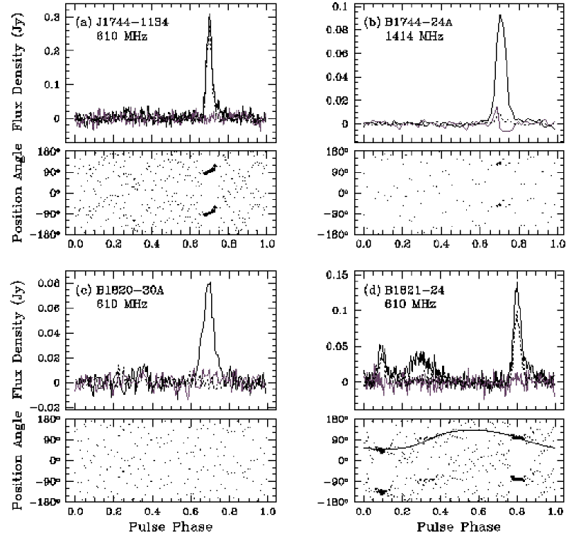
Figure 7: Pulse profiles for (a) PSR J1744$-$1134 at 610 MHz, (b) PSR B1744$-$24A at 1414 MHz, (c) PSR B1820$-$30A at 610 MHz, (d) PSR B1821$-$24 at 610 MHz. See Figure 1.

PSR B1744$-$24A, in the globular cluster Terzan 5, is a rare eclipsing pulsar. In Figure 7(b) we present the profile resulting from 330 minutes of observations acquired on four separate days and at a wide range of orbital phases; these averaged data yield a maximum linear polarization of 9%. Our observations do not support the result of Xilouris et al. (1998), who found a linear polarization fraction of 60%. The data of Xilouris et al. (1998) were taken during a single observing session (Xilouris (1998)); although we saw no similar results in our four days’ observations, it is possible that the linear polarization of 1744-24 is variable.

4.9 PSR B1821$-$24

The pulse profile is complex, with multiple components and strong linear intensity in at least two components. The position angle is nearly flat across the individual components, though there are offsets between components which are not consistent with orthogonal mode changes. We find a possible RVM fit for the position-angle swing, with $\alpha=40.7\pm 1.7^{\circ}$, $\beta=40\pm 10^{\circ}$. Our result is consistent with the estimate of $\alpha=50^{\circ}$, $\beta=40^{\circ}$ given in Backer and Sallmen (1997), though the phase of steepest swing is offset by roughly $180^{\circ}$. However, when both $\alpha$ and $\beta$ are near $45^{\circ}$, the RVM curve is nearly symmetric, thus this discrepancy is not as important as it may seem. We find no evidence in our 610 MHz data for mode-changing as described in Backer and Sallmen (1997); however, Backer and Sallmen found no such mode-changes below 1395 MHz.

4.10 PSR J1911$-$1114

There is some frequency evolution apparent in the presented profiles: a trailing component becomes stronger at 610 MHz than at 410 MHz, and there is a reduction in the intensities of both linear and circular polarizations. The strong circular polarization is indicative of a core component, and the small trailer may be a conal outrider. Taken together, the polarization and the frequency development suggest that this MSP may fit into the classification scheme based on slower pulsars. The position angle shows orthogonal mode switching at both frequencies.

4.11 PSR B1937$+$21

This isolated object was the first millisecond pulsar discovered (Backer et al. (1982)), and it is still the fastest known. Its polarimetric properties have previously been studied at multiple frequencies (Stinebring (1983); Stinebring & Cordes (1983); Ashworth, Lyne, & Smith (1983); Stinebring et al. 1984a ; Thorsett & Stinebring (1990); Sallmen (1998)). Our results agree well with those published earlier, and offer considerable information about the position angle behavior at the leading edge of the main pulse at 1414 MHz. The main-pulse peak linear polarization decreases from 75% at 610 MHz to 49% at 1414 MHz; the position angle is nearly flat across both the main pulse and the interpulse, with evidence for orthogonal mode changes at the leading edge of the main pulse at 1414 MHz and of both components at 610 MHz. Both components broaden as a result of scattering at lower frequencies. As the main pulse and interpulse are separated by nearly $180^{\circ}$ of phase, it is sensible to interpret the emission as coming from an orthogonal rotator. As mentioned in Thorsett and Stinebring (1990), the observed pulse widths are much narrower than those predicted by the empirical relation between the spin period and magnetic inclination (Rankin (1990)).

4.12 PSR J2145$-$0750

The profile of this IMBP contains at least three components, with bridged emission between the two strongest. There is considerable frequency evolution: the main pulse component strengthens relative to the others at higher frequencies. Along with the sense-reversing circular polarization in the last component, this suggests that the last component is core emission, while the “main pulse” is conal. However, it is not clear how to interpret the precursor in this picture. The linear intensity is strongest at low frequencies, and the accompanying position-angle swing is extremely complex, with multiple orthogonal mode changes. Even with the mode changes subtracted, the RVM is not a good fit to the 410 MHz or 610 MHz profiles. At 1414 MHz, we find that the linear intensity drops to very low levels. In contrast, Xilouris et al. (1998) present a profile with reasonably strong linear polarization and a shallow position-angle swing. Sallmen (1998) reports a similar profile (strong linear intensity, shallow position-angle swing) derived from a single observation at 820 MHz at Green Bank. It seems therefore that the linear emission is highly variable, further challenging models of the pulsar emission mechanisms.

5 Conclusion

Millisecond pulsars share a number of polarization characteristics with slow pulsars; in particular, high degrees of linear and circular polarization, well-defined position-angle swings, and orthogonal mode switching appear to be common in both classes. However, very few MSPs have profiles which evolve following the predictions of the slow-pulsar phenomenological model or have position-angle swings which fit the rotating vector model. Our results add to the evidence that recycled pulsars have more complex polarimetric properties than younger pulsars.

Figure 1: Pulse profiles for (a) PSR B1929+10 at 410 MHz, (b) PSR B1929+10 at 610 MHz, (c) PSR B1929+10 at 1414 MHz, (d) PSR J0034$-$0534 at 410 MHz. The solid black line represents the total intensity S, the dotted black line the linear intensity L, and the solid gray line the circular intensity V. The position angle $\psi$ is plotted twice for clarity; larger points are used when L is more significant. The curves indicate the fits to the rotating vector model.

Figure 2: Pulse profiles for (a) PSR J0218+4232 at 410 MHz, (b) PSR J0218+4232 at 610 MHz, (c) PSR J0613$-$0200 at 410 MHz, (d) PSR J0613$-$0200 at 610 MHz. See Figure 1.

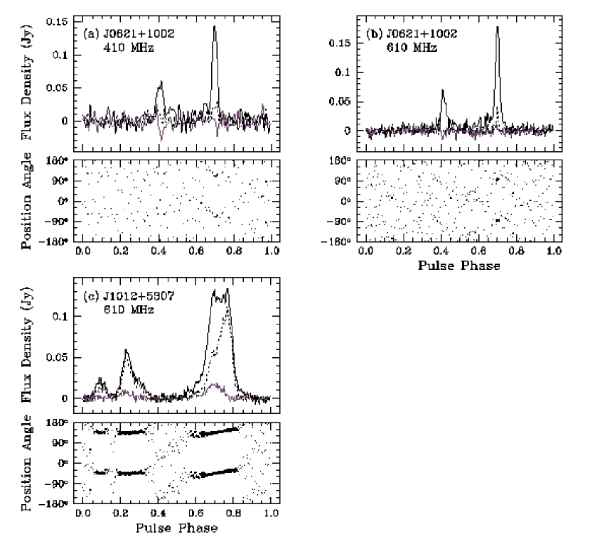
Figure 3: Pulse profiles for (a) PSR J0621+1002 at 410 MHz, (b) PSR J0621+1002 at 610 MHz, (c) PSR J1012+5307 at 610 MHz. See Figure 1.

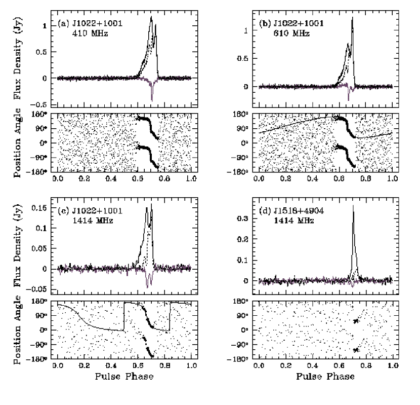
Figure 4: Pulse profiles for (a) PSR J1022+1001 at 410 MHz, (b) PSR J1022+1001 at 610 MHz, (c) PSR J1022+1001 at 1414 MHz, (d) PSR J1518+4904 at 610 MHz. See Figure 1.

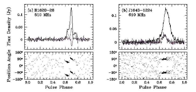
Figure 5: Pulse profiles for (a) PSR B1620$-$26 at 610 MHz, (b) PSR J1643$-$1224 at 610 MHz. See Figure 1.

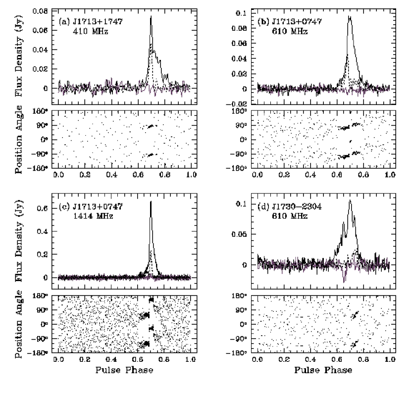
Figure 6: Pulse profiles for (a) PSR J1713+0747 at 410 MHz, (b) PSR J1713+0747 at 610 MHz, (c) PSR J1713+0747 at 1414 MHz, (d) PSR J1730$-$2304 at 610 MHz. See Figure 1.

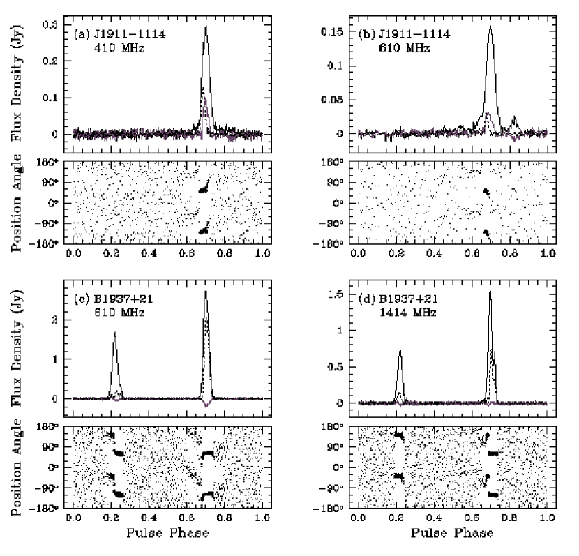
Figure 8: Pulse profiles for (a) PSR J1911$-$1114 at 410 MHz, (b) PSR J1911$-$1114 at 610 MHz, (c) PSR B1937+21 at 610 MHz, (d) PSR B1937+21 at 1414 MHz. See Figure 1.

Figure 9: Pulse profiles for (a) PSR J2051$-$0827 at 410 MHz, (b) PSR J2051$-$0827 at 610 MHz. See Figure 1.

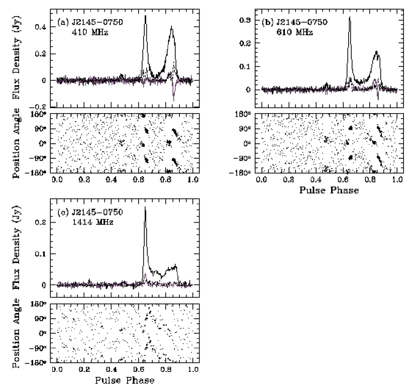
Figure 10: Pulse profiles for (a) PSR J2145$-$0750 at 410 MHz, (b) PSR J2145$-$0750 at 610 MHz, (c) PSR J2145$-$0750 at 1414 MHz. See Figure 1.

Table 1: Rotating vector model fits for PSR B1929$+$10.

Frequency					Phase of Steepest		Reduced
(MHz)	$\alpha$ (∘)		$\beta$ (∘)		PA Slope (∘)		$\chi^{2}$
410	$41$$\pm$	$8$	$21$$\pm$	$4$	$-12.5$$\pm$	$1.0$	1.03
610	$51$$\pm$	$3$	$35$$\pm$	$3$	$-11.2$$\pm$	$1.4$	1.00
1414	$61$$\pm$	$2$	$39$$\pm$	$2$	$-5$$\pm$	$2$	1.02

Table 2: Pulsars observed at Jodrell Bank.

Pulsar	$P$	$\dot{P}$	$\log B$	$\log\tau_{\rm c}$	Reference
	(ms)	($10^{-18}$)	(G)	(yr)
J0034$-$0534	1.88	0.0051	8.00	9.77
J0218$+$4232	2.32	0.08	8.64	8.66
J0613$-$0200	3.06	0.0096	8.24	9.70
J0621$+$1002	28.85	0.04	9.04	10.06	1,2
J1012$+$5307	5.26	0.015	8.45	9.74
J1022$+$1001	16.45	0.04	8.91	9.81	1
J1518$+$4904	40.93	0.027	9.03	10.38	3
B1620$-$26	11.08	0.82	9.48	8.33
J1643$-$1224	4.62	0.018	8.47	9.61
J1713$+$0747	4.57	0.0085	8.30	9.93
J1730$-$2304	8.12	0.020	8.61	9.81
J1744$-$1134	4.07	0.0086	8.28	9.87	4
B1744$-$24A	11.56	$-$0.019
B1820$-$30A	5.44	3.38	9.64	7.41
B1821$-$24	3.05	1.61	9.35	7.48
J1911$-$1114	3.63	0.013	8.34	9.65	5
B1937$+$21	1.56	0.11	8.62	8.35
J2051$-$0827	4.51	0.013	8.39	9.74	6
J2145$-$0750	16.05	0.030	8.85	9.93	2

Table 3: Parameters of polarimetry observations.

Pulsar	Frequency	Resolution	Integration time	Integration time	Previous
	(MHz)	($\mu$s)	(profile) (min)	(flux) (min)	Polarimetry
J0034$-$0534	410	15	180	270
J0218$+$4232	410	36	60	60
	610	36	180	300
J0613$-$0200	410	12	180	180
	610	12	90	150	1
J0621$+$1002	410	225	30	30
	610	113	60	90
J1012$+$5307	610	21	300	360	1
J1022$+$1001	410	16	30	30	2
	610	16	30	180	1
	1414	64	50	185	1,3
J1518$+$4904	610	160	20	20
B1620$-$26	610	87	60	120	1
J1643$-$1224	610	18	90	90
J1713$+$0747	410	36	240	240
	610	18	300	390	1
	1414	4	30	140	1,3
J1730$-$2304	610	32	120	120	1
J1744$-$1134	610	16	30	30
B1744$-$24A	1414	181	330	420	3
B1820$-$30A	610	42	90	90
B1821$-$24	610	12	90	90	1,4
J1911$-$1114	410	7	270	270
	610	14	210	330
B1937$+$21	610	1.5	90	250	1
	1414	1.5	105	620	1,5
J2051$-$0827	410	18	110	140
	610	35	120	300
J2145$-$0750	410	31	60	60
	610	31	120	120	1
	1414	63	30	130	1,3

Table 4: Pulse widths, mean polarization intensities and mean fluxes.

Pulsar	Frequency	$w_{50}$	$w_{10}$	$w_{\rm e}$	Mean	Mean	Mean
	(MHz)	(mP)	(mP)	(mP)	L (%)	$|$V$|$ (%)	Flux (mJy)
J0034$-$0534	410	344	524	266	0	18	24
J0218$+$4232	410	452		477	24	5	47
	610	435		423	22	4	22
J0613$-$0200	410	34	327	75	20	28	9.2
	610	30	315	72	22	24	6.9
J0621$+$1002	410	31		63	13	39	9.5
	610	24	352	55	6	22	9.3
J1012$+$5307	610	137		193	61	12	24
J1022$+$1001	410	69	137	72	70	13	75
	610	56	124	51	71	10	22
	1414	66	132	73	40	25	5.3
J1518$+$4904	610	17	55	27	17	17	8.7
B1620$-$26	610	39	176	72	30	26	9.0
J1643$-$1224	610	117	436	129	12	22	16
J1713$+$0747	410	42		71	27	29	6.8
	610	61	210	78	26	12	6.8
	1414	24	92	37	22	7	7.9
J1730$-$2304	610	97	322	97	11	21	11
J1744$-$1134	610	33	82	46	64	19	13
B1744$-$24A	1414	59	112	63	7	14	4.6
B1820$-$30A	610	63	180	78	0	18	7.1
B1821$-$24	610	42		113	41	26	17
J1911$-$1114	410	45	91	51	20	24	15
	610	51	125	68	7	19	8.1
B1937$+$21	610	35	56	57	42	5	131
	1414	24	55	44	29	3	24
J2051$-$0827	410	48	252	75	8	15	7.9
	610	98	296	127	1	18	4.2
J2145$-$0750	410	234	265	96	13	14	46
	610	215	261	80	11	17	19
	1414	21	261	67	5	18	6.6

Table 5: Rotating vector model fits

Pulsar	Frequency							Phase of Steepest			Reduced
	(MHz)	$\alpha$ (∘)			$\beta$ (∘)			PA Slope (∘)			$\chi^{2}$
J0218$+$4232	410	$8$	$\pm$	$11$	undetermined			$-39$	$\pm$	$5$	0.87
	610	$8$	$\pm$	$15$	undetermined			$-45$	$\pm$	$5$	1.03
J1022$+$1001	610	$140$	$\pm$	$16$	$-4.9$	$\pm$	$1.8$	$-12.2$	$\pm$	$0.2$	1.06
	1414	$83$	$\pm$	$27$	$-7.1$	$\pm$	$0.4$	$-13.3$	$\pm$	$0.5$	1.04
B1821$-$24	610	$40.7$	$\pm$	$1.7$	$40$	$\pm$	$10$	$-167.1$	$\pm$	$1.9$	1.04