Cloning Hubble Deep Fields II: Models for Evolution
by Bright Galaxy Image Transformation

Abstract

In a companion paper we outlined a methodology for generating parameter-free, model-independent “no-evolution” fields of faint galaxy images, demonstrating the need for significant evolution in the HDF at faint magnitudes. Here we incorporate evolution into our procedure, by transforming the input bright galaxy images with redshift, for comparison with the HDF at faint magnitudes. Pure luminosity evolution is explored assuming that galaxy surface brightness evolves uniformly, at a rate chosen to reproduce the I-band counts. This form of evolution exacerbates the size discrepancy identified by our no-evolution simulations, by increasing the area of a galaxy visible to a fixed isophote. Reasonable dwarf-augmented models are unable to generate the count excess invoking moderate rates of stellar evolution. A plausible fit to the counts and sizes is provided by ‘mass-conserving’ density-evolution, consistent with small-scale hierarchical growth, where the product of disk area and space density is conserved with redshift. Here the increased surface brightness generated by stellar evolution is accomodated by the reduced average galaxy size, for a wide range of geometries. These models are useful for assessing the limitations of the HDF images, by calculating their rates of incompleteness and the degree of over-counting. Finally we demonstrate the potential for improvement in quantifying evolution at fainter magnitudes using the HST Advanced Camera, with its superior UV and optical performance.

&

1 Introduction

Deep HST images have proven difficult to interpret. One might have imagined that clear pictures of the distant Universe would speak for themselves, revealing directly how galaxies formed and evolved. Instead, interpretation has been hampered by our ignorance of the UV properties of local galaxies. In a companion paper (Bouwens, Broadhurst, & Silk 1998; BBS-I), we showed how this problem can be overcome using a redshift-complete sample of bright galaxies contructed from the UV-optical HDF images and follow-up spectroscopy. Clear evolutionary trends were identified by projecting this bright sample to much fainter magnitudes in a purely empirical and model-independent way. In the present paper, we explore simple models for evolution by modifying our procedure to generate realistic deep fields for exploring the question of evolution to magnitudes far fainter than accessed by spectroscopy. We commence with nearby galaxies and project them back into the past, modifying the number, surface brightness and sizes of the images in ways designed to embody both luminosity and density evolution and to explore the possible role of dwarf galaxies. These simple image transformation models represent a heuristic alternative to other more complicated evolutionary approaches with more model-dependent and parameter-laden representations of galaxies at both low and high redshift.

At present this empirical modelling is still a more reliable guide to the process of galaxy evolution than that derived from numerical work in the context of the hierarchical models for the growth of structure. High-resolution codes which simulate the gravitational interactions of gas and cold dark matter and incorporate cooling following standard atomic physics produce small, dense and rapidly rotating disks in the center of massive haloes (Navarro & White 1994; Navarro & Steinmetz 1997). Of course, ad-hoc heat input from supernovae can presumably be added to achieve larger disks, but, nonetheless, even with this level of freedom, the rotation curves of dwarf galaxies such as DDO154 (Carignan & Freeman 1988) and other newly discovered dwarfs (Cote, Freeman, & Carignan 1997) defy simple explanation (Navarro, Frenk, & White 1996; Burkert & Silk 1997). Semi-analytic attempts to mock up hierarchical evolution (cf. Baugh, Cole, & Frenk 1996; Kauffmann, Guiderdoni, & White 1994), though providing interesting interpretations through which to understand the various observables relevant to galaxy formation and evolution, still include many free parameters. Improved modelling of the observations will undoubtedly require a deeper understanding of the interplay of physical processes relevant to star formation.

In §1, we describe our models for evolution and compare them with the HDF observations in §2. In §3, we discuss the results, and in §4 we present our conclusions and discuss future prospects. As in BBS-I, we adopt $H_{0}=50\,\textrm{km/s/Mpc}$ and express all magnitudes in this paper in the AB magnitude system (defined in terms of a flat spectrum in frequency). Also, to associate the HDF bands with their more familiar optical counterparts, we shall refer to the $F814W$, $F606W$, $F450W$, and $F300W$ bands as $I_{814}$, $V_{606}$, $B_{450}$, and $U_{300}$, respectively, throughout this paper.

2 Standard Models

We present simple augmentations to our procedure for generating realistic deep fields as described in detail in BBS-I. We incorporate the usual phenomenological models proposed to explain the number counts: pure luminosity evolution, “mass-conserving” density evolution, and the contribution of an evolving low-luminosity (dwarf) population, all of which have been claimed to be important for matching the number counts at faint magnitudes. We proceed by performing simple scalings of the images of our bright HDF galaxy sample (see BBS-I) in surface brightness, size, and the space density in the simplest manner possible in order to achieve rough agreement with the number counts in the $I_{814}$ band.

Unfortunately, by virtue of its size, our bright HDF sample lacks low luminosity galaxies, and therefore dwarfs are necessarily included in an ad-hoc manner, requiring that we specify in addition to their evolution their image profiles and luminosity functions. This latitude has generated a large literature on their potential contribution (Kron 1982; Cowie, Songaila, & Hu 1991; Gronwall & Koo 1995; Ferguson & McGaugh 1995; Driver & Phillips 1996). In the present work, we have chosen to consider a somewhat conservative “maximal” estimate of this contribution, using constraints on the faint end slope of the LF from recent redshift surveys.

2.1 Luminosity Evolution

To obtain a rough idea of the effect of luminosity evolution on deep field images, we modify our simulation procedure to include a simple $(1+z)^{b}$ scaling in surface brightness, a very simple prescription for obtaining fair agreement with the number counts in the $I_{814}$ band to some specified magnitude limit. Of course, one could model this form of evolution with more sophistication using the usual assumptions (Pozzetti, Bruzual, & Zamorani 1996; Ferguson & Babul 1998), even implementing it on a pixel-by-pixel basis where the observed pixel colours could be used to model the spatial history of star formation. However, we have decided not to pursue this here because of the many additional assumptions required and the simple fact that such models, as we will illustrate, would inevitably seem to produce galactic populations with sizes that are too large. In BBS-I, such a trend toward small sizes was already evident.

2.2 Density Evolution

To estimate the manner in which density evolution would alter the predictions of our empirical no-evolution method, for simplicity, we have chosen to scale the number densities of each bright galaxy in the sample as $(1+z)^{Q}$ without changing their relative proportions. To make this simple model sensible, we decrease the metric sizes subject to the simple constraint that the integrated mass is preserved, similar to the models proposed by Rocca-Volmerange & Guiderdoni (1990) and Broadhurst, Ellis, & Glazebrook (1992). For disk galaxies, this simply translates into the requirement that galaxies change in area at a rate, $(1+z)^{-Q}$, inversely proportional to the space density evolution. As discussed in Broadhurst et al. (1992), it is also necessary in the context of this simple “merger” prescription to add luminosity evolution, since otherwise the number counts are virtually unaffected. We also parameterize this luminosity evolution as a $(1+z)^{b}$ scaling.

We shall avoid consideration here of various arguments against this scenario, for which high rates of merging are claimed to be problematic (Tóth & Ostriker 1992, Lacey & Cole 1993; Dalcanton 1993; Roukema & Yoshii 1993), recognising that from a purely empirical perspective this model has considerable intrinsic appeal.

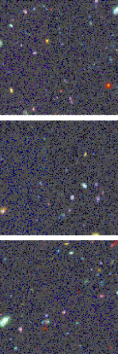
Figure 1: Panel (a) shows a simulated 96” x 46” colour image generated from the $B_{450}$, $V_{606}$, and $I_{814}$ bands for our $\Omega=0.1$/$\Lambda=0.9$ LE prescription with $\Omega=1$ constructed with pixel size, signal-to-noise, and PSF identical to that of the HDF. Panels (b) and (c) is similar to panel (a), except using the $\Omega=0.1$ and $\Omega=1.0$ LE prescriptions, respectively. All LE models produce objects which are larger on average than the data. Also note prominent examples of objects breaking-up into HII regions at high redshift apparent in several panels.

For both the luminosity evolution and density evolution models, we have listed the best-fit parameters in Table 1. Except for simple scalings in number density, size, and surface brightness, we performed these simulations in an identical manner to that described in BBS-I using the Coleman, Wu, & Weedman (1980) SED templates. Note that we self-consistently derived $V_{max}$ and the number densities for each geometry and evolutionary scenario. For the purposes of illustration, we present our pure luminosity simulations in Figure 1 for three different geometries ($\Lambda=0.9$/$\Omega=0.1$; $\Omega=0.1$; $\Omega=1$) and an HDF density evolution simulation in Figure 2.

2.3 Low-Luminosity Galaxies

Currently, our input bright galaxy sample does not extend faintward of $M_{b_{j}}=-18$. Consequently, we have included a model low-luminosity population to explore the potential role of a dwarf population. Such a model is particularly important to explore since it is well understood that in the absence of evolution, the low-luminosity galaxies comprise an increasing contribution to the counts at faint magnitudes by virtue of their relatively small k-corrections and the increasing volume available to these galaxies relative to the more luminous galaxies, particularly for large $\Omega$ (Kron 1982).

Given the latitude of possible models permissible for the low luminosity galaxies, we shall simply use the same luminosity function, initial mass functions (IMF) and star formation histories as are given in the Pozzetti et al. (1996) pure luminosity evolution model for the Sabc and Sdm spectral types, except that we shall adopt a normalization which is 50% higher than the value prescribed in Pozzetti et al. (1996) and we truncate the luminosity function at absolute magnitudes $b_{j}<-18$, brightward of which our bright HDF sample (see BBS-I) is well-represented. Our low-luminosity population already overproduces the low-redshift galaxies in the CFRS, but might be tolerated depending on where this survey’s 19% incompleteness lies in redshift. These dwarfs are all endowed with exponential profiles with a $b_{j}=22.65\,\textrm{mag/arcsec}^{2}$ central surface brightness. We have intentionally chosen a central surface brightness lower than the commonly observed central surface brightness of 21.65 $b_{j}\,\textrm{mag/arsec}^{2}$ typical of high luminosity objects, as a way to conservatively account for the claimed correlation between surface brightness and luminosity (McGaugh & de Blok 1997). A summary of the parameters used in this model is provided in Table 2.

Although there continues to be debate about the importance of low luminosity galaxies, both locally and in the past, we feel that our treatment of dwarfs is generous, pushing the limits of what is supported by observation. Relative to other determinations of the local field galaxy luminosity function, we have a fairly high normalization and a relatively steep faint-end slope $-1.24$, much like the LF claimed by the fairly deep ESP survey of Zucca et al. (1997) and steeper than the well defined APM luminosity function of Loveday et al. (1992). At fainter magnitudes, no redshift survey has ever shown as many low redshift objects as one would expect if the density of dwarfs was much larger than this (Broadhurst, Ellis, & Shanks 1988; Glazebrook et al. 1995a; Cowie et al. 1996; Lilly et al. 1995; Ellis et al. 1996; Heyl et al. 1997). Indeed, with regard to the observed distribution of redshifts from the CFRS, our generous model for the low-luminosity population of galaxies already generates a $\sim 50\%$ excess at the low redshift end. Despite these constraints, a larger population of dwarfs could in principle be admitted within these observational constraints by adopting a much steeper slope to the luminosity function, a possibility for which there has been some recent support (Loveday 1997).

For this model, we have generated Monte-Carlo catalogues and simulated images in $U_{300}$, $B_{450}$, $V_{606}$, and $I_{814}$, equal in area to 4 times that of the HDF. The dwarfs are placed on the image at random positions and inclination angles, assuming no extinction and smoothed with an unsaturated, relatively isolated stellar PSF taken from the HDF. Then both poissonian and sky noise are placed on the images, after applying the noise kernel to reproduce the drizzled properties of the noise. We calculate the colours for these galaxies with their chosen star-formation histories using a recent version of the Bruzual & Charlot spectral synthesis tables, compiled in Leitherer et al. (1996) (see Charlot, Worthey, & Bressan 1996 for a description of these type of models.) We recover objects off the resulting dwarf-augmented images using SExtractor in exactly the same manner that we recover objects from the HDF.

3 Results

3.1 Number Counts in the $I_{814}$ band

As in BBS-I, we begin by examining the number counts derived from the above models in the $I_{814}$ band due to relatively small uncertainties inherent in determining the fluxes each of the input galaxies would have to $z\sim 3$ in this band. The pure bolometric luminosity evolution results are presented in Figure 3 as a dashed line. The rate, parameterized as $(1+z)^{b}$, ranges over $b=1.4-2.5$ depending on the geometry, being smaller for models with larger volume elements. At the faintest magnitudes, the model counts fall off with respect to the data, a feature more the result of a higher level of incompleteness than a lack of volume at high redshift. Incompleteness sets in because the higher mean redshifts generated with this form of evolution results in a lower mean surface brightness at high redshift, where the rate of cosmological dimming $(1+z)^{4}$ is much greater than the compensation from luminosity evolution. Note that these rates of luminosity evolution are roughly consistent, albeit a little lower than the best fit found by Lilly et al. (1998) of $(1+z)^{2.7}$ for the spiral galaxy population ($\Omega=1$, $0\lesssim z\lesssim 1$).

For “mass-conserving” density evolution (shown in Figure 3 as a solid line) we require a fairly high rate of density-evolution, $(1+z)^{Q}$, where $Q=4-4.5$ and a milder rate of luminosity evolution $(1+z)^{b}$ than above where $b=0.2-1.2$ in order to approximately reproduce both the number counts and the angular sizes. With the specified large merging rate and a consequently larger number density at moderately high redshifts ($z>1$), it is trivial to reproduce the observed number of galaxies in the HDF. Furthermore, with suitable adjustments of the relative amounts of luminosity and density evolution ($Q/b$), it is possible to simultaneously produce a rough fit to the angular size distributions as well for any choice of $\Omega$ (Figure 4).

3.2 Angular Sizes

We compare the distributions of half-light radii recovered from the HDF with those of our simulations in Figure 4. Clearly, at bright magnitudes ($21<I_{814,AB}<22.6$), the angular sizes recovered from the simulations agree well with the observations as expected given the selection of our input prototypes from this same magnitude range. However, at fainter magnitudes, the half-light radii from the no-evolution simulations (hatched area in Figure 4 indicating the 1 $\sigma$ uncertainty based on the size of the bright sample) are significantly larger than for the observations being somewhat reduced for the cases of lower $\Omega$ (see BBS-I). Adding our ad-hoc dwarf population (shown in Figure 4 as a dotted line) to the no-evolution results, we still recover $3.6\pm 1.2$, $4.5\pm 1.3$, and $8.1\pm 2.2$ times fewer objects than we recover in the HDF for the size interval 0.15 arcsec $<r_{hl}<$ 0.2 arcsec and magnitude interval $24<I_{814,AB}<26$ for $\Lambda=0.9$/$\Omega=0.1$, $\Omega=0.1$, and $\Omega=1.0$, respectively.

Incorporating our pure luminosity prescription (shown in Figure 4 as a dashed line) only worsens the situation. Not only are the recovered angular size distributions much larger than those observed, but also the number of large galaxies recovered is clearly in excess of the data. This significant shift to larger sizes results from the general shift to higher redshifts and hence lower surface brightness at fixed magnitude where the $(1+z)^{4}$ cosmological dimming wins over the $(1+z)^{1.4-2.5}$ surface brightness evolution required to enhance the predicted counts.

Therefore, unless we have greatly erred in constraining the properties of the dwarf population, it seems clear that a large fraction of faint galaxies are intrinsically smaller than our low-redshift input galaxy sample. Accordingly, it is not surprising that our mass-conserving density evolution prescription is quite successful in allowing us to match the observed sizes, while at the same time allowing us to easily match the total number of galaxies observed to a given magnitude limit (Figure 3). For this two-parameter model, the range of $Q$ and $B$ which fit both the counts and the sizes is moderately well-constrained by the data. The counts are most sensitive to $B$, and the sizes to $Q$, allowing us some independence in deriving the rates.

3.3 Completeness and Overcounting

Since we can easily match up our input generated catalogue with the recovered properties of galaxies (see BBS-I), it is simple to determine quantities like the incompleteness. Figure 5 shows that the incompleteness becomes significant in the range $I_{814,AB}>26$ for both our no-evolution simulations and those based on our simple luminosity evolution prescriptions. Incompleteness results from the fact that at increasingly faint magnitudes, detection requires smaller and hence intrinsically higher surface brightness galaxies at fixed magnitude. Consequently the merger and dwarf models suffer less incompleteness at a given magnitude because of their inherently smaller sizes. Of course, evaluating the incompleteness is ultimately model-dependent, but the gentle rollover at faint magnitudes occurs in a very similar way for our merger model as in the HDF, consistent with our finding above that the faint galaxies have small intrinsic angular sizes.

In a similar manner, we determine the rate at which we overcount the galaxy population in our simulated fields since each image detected can be traced back to only one galaxy in the input catalogue. In Figure 6, we display the rate of overcounting for all the simulations performed. Evidently, in our simulations, overcounting is never an important effect. The worst case is for luminosity evolution, especially the $(1+z)^{2.5}$ brightening rate used in the $\Omega=1$ geometry. With this form of evolution the redshift distribution extends to high redshifts ($z\sim 2-5$), where the bright ultraviolet light of the HII regions clearly stands. Several prominent examples of these galaxies are evident in the simulated images (see Figure 1).

3.4 Redshift Distributions

In Figure 7, we plot the predicted redshift distributions of the galaxies recovered by matching up those objects recovered by SExtractor with our input catalogues. Without evolution, very few galaxies lie beyond a redshift $z=2$, even at the faintest magnitudes. Similarly, for our density-evolution models, galaxies also have rather low redshifts, a direct consequence of the increasingly small sizes and luminosities of galaxies in this prescription. In contrast, luminosity evolution accesses much higher redshifts as individual objects are enhanced in luminosity.

3.5 $U_{300}$ and $B_{450}$ “Dropouts”

As in BBS-I, we can compare the number of high-redshift dropout galaxies recovered from our simulations with those found in the HDF. We present the Madau et al. (1996) colour-colour criterion for the $U_{300}$ and $B_{450}$ dropouts in Figures 8-9 and tabulate the number identified in Table 3.

As in our no-evolution simulations (see BBS-I), our simple merging prescription underpredicts the numbers of $U_{300}$ and $B_{450}$ band dropouts. Of course, with luminosity evolution, the numbers of dropouts are higher. Clearly, a more realistic inclusion of the star formation activity in these models and the subsequent shift of the bolometric flux into the ultraviolet would further serve to increase the number of high redshift objects in both the pure luminosity and density evolution models. Taking this into account, we might expect to find an excess of dropouts in our luminosity evolution model, similar to the findings of Ferguson & Babul (1998) and Pozzetti et al. (1998), as well as a larger number of dropouts in our density evolution model.

4 Advanced Camera

We can use our simulations to predict the likely quality of even deeper images to be obtained using the HST Advanced Camera. Its Wide Field Camera (WFC) promises to have a throughput which is $\sim 3.5$ greater than the peak thoughtput of WFPC2 at $\sim 6500$ $\AA$, $\sim 5$ greater in the $B$ band ($\sim 4500$ $\AA$), and $\sim 7$ greater in the $Z$ band ($\sim 9000$ $\AA$). Figure 2 shows a direct comparison of the image quality of WFPC2 (HDF depth) with that obtainable with the AC (simply using the improved response) where our preferred $\Omega=1$ density evolution model is used for the simulation. In addition to the nominal $0.^{m}7$ to $1.^{m}1$ improvement in depth due to the increased sensitivity, the field of view of the WFC will be 200” x 204”, twice as large as WFPC2, with a pixel scale half as small so that by drizzling (not included here) further improvements in resolution and therefore depth (for the smallest objects) are expected.

In addition, since we are currently limited by the lack of good UV images, the High Resolution Camera (HRC) of the Advanced Camera, though of more limited area coverage (26” x 29”), will in principle provide a much large sample of UV-optical imaged galaxies from which to expand an input prototype sample, such as was used in the present work. The UV performace is 10 times higher than WFPC2 (Ford et al. 1997) at $2000\AA$ and extends from $2000\AA$ to $10000\AA$. In light of this superior performance from the UV to the optical, the Advanced Camera should furthermore be quite powerful in identifying a large drop-out population up to and through the $V$ band.

5 Discussion

Our most interesting finding here relates to the sizes of the faint images. The sizes are smaller in projected areas than our no-evolution extrapolation of the input bright galaxy sample ($\bar{z}\sim 0.5$). Adding in simple luminosity evolution only makes the situation worse, particularly for high $\Omega$ as sizes then effectively become larger than in the NE model. This, together with the lack of bright blue E/SO galaxies, make it hard to accept the traditional view that the observed evolution is merely dominated by the stellar evolution. It is easier to accommodate the size evolution and count excess by dropping the usual assumption of space-density conservation and replacing it with the more general and physically motivated idea that mass is conserved. A realistic merger model, involving star formation induced during gas-rich mergers is needed to fully develop this approach. For simplicity, we have chosen to present a cruder model that nevertheless reveals the general effect. Here we have traded image size for space density, so that the product is independent of redshift, which for disk galaxies approximates mass conservation. Although we underpredict the fraction of dropouts, a more realistic attempt to mock up this form of evolution would include the enhancement in luminosity associated with the starburst phase which is well documented from local examples of merging and interacting galaxies (e.g. Joseph et al. 1984). A self-consistent modification of this model can be imagined which might draw on the observed evolution of the blue starburst population observed in the field and its continuation to high redshift found by Cowie et al. (1996) and Steidel et al. (1996).

Contrary to our conclusion regarding the HDF, Ferguson & Babul (1998) find in their modeling of luminosity evolution that the size distribution of the faint galaxy population observed is consistent with a low $\Omega$ Universe. Ferguson & Babul (1998) do not evolve the physical sizes of their galaxies and base their input parameters on local galaxy observations. Whilst we are not completely sure of the source of this disagreement, we suspect that the surface brightnesses and normalizations they use for the lowest luminosity objects may be too high relative to observations (cf. McGaugh & de Blok 1997). In any case, we are inclined to place greater weight on our finding because of our direct use of real two-dimensional images for a complete sample of galaxies.

6 Conclusions

Pure evolution in luminosity and hence in surface brightness can be made to match the number-count excess for geometries with large volume elements (i.e. $\Lambda=0.9$/$\Omega=0.1$). Unfortunately, such models reveal a discrepancy in terms of the angular sizes of the faint galaxy population. Clearly, galaxies would seem to evolve such that their sizes become intrinsically smaller as well as more numerous. “Mass-conserving” density evolution (merging) can easily be made to achieve this goal, but at the expense of lowering the mean redshift and thereby underpredicting the observed “dropout” rate in the $U_{300}$ and $B_{450}$ bands. This problem might be somewhat alleviated by accounting for the expected shift in bolometric luminosity during the merger of gas rich systems. Consequently, it might be worth pursuing in more detail the effect of starburst activity on the appearance and pixel-by-pixel spectral energy distribution of the sample in question. Dwarfs can also be added, but the low-redshift constraint on their frequency is such that they would have to have an extremely steep slope or rapid evolution, neither of which appear supported by current observations.

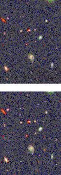
Figure 2: Panel (a) shows a simulated 100” x 64” colour image generated from the $B_{450}$, $V_{606}$, and $I_{814}$ bands for our merging prescription where $L\propto(1+z)^{1}$ and $n\propto(1+z)^{2}$ in a $\Omega=1.0$ geometry, constructed with pixel size, signal-to-noise, and PSF identical to that of the HDF. Both the number counts and angular size distributions are in good agreement with the HDF. Panel (b) shows a similarly-sized region of the same model, except that the sensitivities of the Advanced Camera are used, here estimated to be 5, 4, and 5 times larger than for WFPC2 in the $B$, $V$, and $I$ bands, respectively. Notice the large increase in the number of faint galaxies expected.

Figure 3: A comparison of the observed $I_{814,AB}$-band number counts (histogram with $1\sigma$ Poisson errors) with those recovered from our simple merging prescription (solid line) and our pure luminosity prescription (dashed line). For comparison, the counts recovered from the no-evolution simulations are shown (the hatched area representing the estimated 1 $\sigma$ range in these counts based on the finite size of our bright input sample) along with those estimated to derive from low-luminosity galaxies (dotted line). All cases are shown for $\Omega=0.1$/$\Lambda=0.9$, $\Omega=0.1$, and $\Omega=1$ geometries. Note that the turnover in the number counts at faint magnitudes ($I_{814,AB}\sim 26$) is more a result of incompleteness than a lack of volume at high redshifts.

Figure 4: A comparison of the observed distribution of half-light radii recovered from the HDF (histogram with $1\sigma$ Poissonian uncertainties) with the distribution of half-light radii recovered from pure luminosity evolution simulations (long dashed line) and density evolution simulations (solid line). For reference, we have included the angular size distribution of no-evolution simulations (hatched region with 1 $\sigma$ uncertainties) and our maximal dwarf model (dotted curve). Clearly, the angular sizes for our luminosity evolution simulations are too large even for low $\Omega$. In contrast, the angular sizes for our merger models provide a rough match to the angular sizes recovered from the data.

Figure 5: The completeness of the $I_{814,AB}$-band counts determined from the simulations for the no-evolution simulations (solid line), the luminosity evolution simulations (dashed line), and the density evolution simulations (dot-dashed line). All models are shown for $\Omega=0.1$/$\Lambda=0.9$, $\Omega=0.1$, and $\Omega=1$. Because surface brightness has a rough inverse proportionality to angular size at a given magnitude, the completeness limit is directly related to the angular sizes of the faint galaxy population in that galaxy populations with smaller angular sizes are more complete at fainter magnitudes.

Figure 6: The % of galaxies which are counted more than once, mostly as a result of the fact that in the UV they break up into distinct pieces. The overcounting rate is relatively low and similar for all models, except for the $\Omega=1$ luminosity evolution prescription where $L\propto(1+z)^{2.5}$. For this model, the overcounting rate is much greater because a large percentage of galaxies in any faint magnitude bin at higher redshifts ($z\sim 2-5$, see Figure 7) break-up into distinct lumps due to the strong differential k-correction over the surface of the galaxy (see Figure 1 for a dramatic illustration of this).

Figure 7: Redshift distribution of those objects recovered by SExtractor from our no-evolution simulations (hatched region indicated $1\sigma$ uncertainties), our luminosity evolution simulations (dashed line), our density evolution simulations (solid line), and our maximal dwarf model (dotted line) with $I_{F814W,AB}<26$ and $I_{F814W,AB}<28$ for $\Omega=0.1$/$\Lambda=0.9$, $\Omega=0.1$, and $\Omega=1$ geometries. The luminosity evolution model produces a long tail to high redshift whereas the no-evolution simulations and density-evolution simulations have few galaxies above $z=2$. For comparison, the upper panel shows the redshift estimates by Lanzetta, Yahil, & Fernandez-Soto (1996) which are lower than the estimates by Mobasher et al. (1996) and higher than those of Sawicki, Lin, & Yee (1997).

Figure 8: Comparison of the $(U_{300}-B_{450})_{AB}$ versus $(B_{450}-I_{814})_{AB}$ diagrams for our no-evolution simulations (lowest panel), our luminosity evolution simulations (second highest panel), and our density evolution simulations (top panel) with the observations for $B_{450,AB}<26.9$ (the same criterion used in Madau et al. 1996). The area interior to the dashed line is the region Madau et al. (1996) suggests is occupied by high-redshift galaxies ($2<z<3.5$) whose Lyman limit crosses the $U_{300}$ passband. Note that galaxies near the top of the colour-colour diagram, i.e., with $(U_{300}-B_{450})_{AB}>4.6$, are simply lower limits on the $(U_{300}-B_{450})_{AB}$ colour. Both the no-evolution simulations and our merging prescriptions underpredict the number of dropouts in this region though the luminosity evolution models seem to do much better in matching these observations.

Figure 9: Comparison of the $(B_{450}-V_{606})_{AB}$ versus $(V_{606}-I_{814})_{AB}$ diagrams for our no-evolution simulations (lowest panel), our luminosity evolution simulations (second highest panel), and our density evolution simulations (top panel) against the observations for galaxies with $V_{606,AB}<28.0$ (the same criterion used in Madau et al. 1996). With a dashed line, we have overplotted the $B$-band dropout region suggested by Madau et al. (1996) for finding high redshift ($3.5<z<4.5$) whose Lyman limit crosses the $B$ bandpass. Note that galaxies near the top of the colour-colour diagram, i.e., with $(B_{450}-V_{606})_{AB}>3.5$, are simply lower limits on the $(B_{450}-V_{606})_{AB}$ colour. Similar conclusions hold as for the $U_{300}$ dropouts.

Table 1: Parameterizations Used For Evolutionary Models given in this work.

Evolution	$\Omega$	$\Lambda$	$B$	$Q$
LE	0.1	0.9	1.4	0
LE	0.1	0	1.5	0
LE	1.0	0	2.5	0
DE	0.1	0.9	0.2	4.0
DE	0.1	0	0.5	4.5
DE	1.0	0	1.2	4.3

Table 2: Model parameters for our estimated low-luminosity galaxy population.

$\Omega$	$\phi_{o}$	$M^{*}_{b_{j}}$	$\alpha$	$\tau$	IMF	$t_{f}$ (Gyr)	$\mu_{0}^{b_{J}}$
0.1	1.73	-21.14	-1.24	$\tau_{10}$	Scalo	16	22.75
	0.81	-21.14	-1.24	cons	Salpeter	16	22.75
1	1.73	-21.14	-1.24	$\tau_{8}$	Scalo	12.7	22.75
	0.81	-21.14	-1.24	cons	Salpeter	12.7	22.75

Table 3: Number of $U_{300}$ and $B_{450}$ dropouts. One $\sigma$ uncertainties are given on all simulated results based on the finite size of our bright sample.

Data set	$U_{300}$ dropouts	${B_{450}}$ dropouts
Observations (Madau et al. 1996)	58	14
Observations (This work)	90	19
NE ($\Omega=0.1$/$\Lambda=0.9$)	$1\pm 1$	$3\pm 2$
NE ($\Omega=0.1$)	$2\pm 1$	$4\pm 3$
NE ($\Omega=1$)	$6\pm 3$	$5\pm 3$
LE ($\Omega=0.1$/$\Lambda=0.9$)	$35\pm 12$	$9\pm 3$
LE ($\Omega=0.1$)	$21\pm 8$	$17\pm 6$
LE ($\Omega=1$)	$55\pm 18$	$33\pm 10$
DE ($\Omega=0.1$/$\Lambda=0.9$)	$1\pm 1$	$1\pm 1$
DE ($\Omega=0.1$)	$1\pm 1$	$2\pm 1$
DE ($\Omega=1$)	$2\pm 2$	$2\pm 2$

References

- Baugh, Cole, & Frenk (1996) Baugh, C., Cole, S., & Frenk, C.S. 1996, MNRAS, 282, L27.
- Bouwens, Broadhurst, & Silk (1998) Bouwens, R.J., Broadhurst, T.J., & Silk, J. 1998, ApJ, submitted (BBS-I).
- Broadhurst, Ellis, & Shanks (1988) Broadhurst, T.J., Ellis, R.S, & Shank, T. 1988, MNRAS, 235, 827.
- Broadhurst et al. (1992) Broadhurst, T.J., Ellis, R.S., Glazebrook, K. 1992, Nature, 355, 55.
- Burkert & Silk (1997) Burkert, A., & Silk, J. 1997, ApJ, 488, L55.
- Carignan & Freeman (1988) Carignan, C., & Freeman, K.C. 1988, ApJ, 332, L33.
- Charlot, Worthey, & Bressan (1996) Charlot, S., Worthey, G., & Bressan, A. 1996, ApJ, 457, 625.
- Coleman, Wu, & Weedman (1980) Coleman, G.D., Wu, C.-C., & Weedman, D.W. 1980, ApJS, 43, 393.
- Cote, Freeman, & Carignan (1997) Cote, S., Freeman, K.C., & Carignan, C. 1997, astro-ph/9704031.
- Cowie, Songaila, & Hu (1991) Cowie, L.L., Songaila, A., & Hu, E.M. 1991, Nature, 354, 460.
- Cowie et al. (1996) Cowie, L.L., Songaila, A., Hu, E.M., Cohen, J.D. 1996, AJ, 112, 839.
- Dalcanton (1993) Dalcanton, J.D. 1993, ApJ, 415, L87.
- Driver & Phillips (1996) Driver, S.P., & Phillips, S. 1996, ApJ, 469, 529.
- Ellis et al. (1996) Ellis, R.S., Colless, M., Broadhurst, T.J., Heyl, J.S., Glazebrook, K. 1996, MNRAS, 280: 235-251.
- Ferguson & McGaugh (1995) Ferguson, H.C., & McGaugh, S.S. 1995, ApJ, 440, 470.
- Ferguson et al. (1998) Ferguson, H.C., & Babul, A., 1998, in press.
- Ford et al. (1996) Ford, H.C., et al. 1996. Proc. SPIE, 2807, 184.
- Glazebrook et al. (1995) Glazebrook, K., Ellis, R.S., Colless, M.M., Broadhurst, T.J., Allington-Smith, J.R., Tanvir, N.R. 1995a, MNRAS, 273, 157.
- Gronwall & Koo (1995) Gronwall, C. & Koo, D. 1995, ApJ, 440, L1.
- Guiderdoni & Rocca-Volmerange (1990) Rocca-Volmerange, B. & Guiderdoni, B. 1990, A&A, 252, 435.
- Heyl et al. (1997) Heyl, J.S., Colless, M., Ellis, R.S., Broadhurst, T.J. 1997, MNRAS, 285, 613-634.
- Joseph et al. (1984) Joseph, R.D., Miekle, W.P.S., Robertson, N.A., & Wright, G.S. 1984, MNRAS, 209, 111.
- Lacey & Cole (1993) Lacey, C., & Cole, S. 1993, MNRAS, 262, 627.
- Lanzetta, Yahil, & Fernandez-Soto (1996) Lanzetta, K.M., Yahil, A., Fernandez-Soto, A. 1996, Nature, 381, 759.
- Leitherer et al. (1996) Leitherer et al. 1996, PASP, 108, 996.
- Lilly et al. (1995) Lilly, S.J., Tresse, L., Hammer, F., Crampton, D., LeFevre, O. 1995, ApJ, 455, 108.
- Lilly et al. (1998) Lilly, S.J., et al. 1998, in press.
- Loveday (1997) Loveday, J. 1997, ApJ, 489, 29.
- Kauffmann, Guiderdoni, & White (1994) Kauffmann, G., Guiderdoni, B., & White, S.D.M. 1994, MNRAS, 267, 981.
- Kron (1982) Kron, R.G. 1982, Vistas Astr., 26, 37.
- Madau et al. (1996) Madau, P., Ferguson, H.C., Dickinson, M.E., Giavalisco, M., Steidel, C.C., & Fruchter, A. 1996, MNRAS, 283, 1388.
- McGaugh & de Blok (1997) McGaugh, S.S., & de Blok, W.J.G. 1997, ApJ, 481, 689.
- Mobasher et al. (1996) Mobasher, B., Rowan-Robinson, M., Georgakakis, A., Eaton, N. 1996, MNRAS, 282, L7.
- Navarro & White (1994) Navarro, J.F., & White, S.D.M. 1994, MNRAS, 267, 401.
- Navarro, Frenk, & White (1996) Navarro, J., Frenk, C.S., & White, S.D.M. 1996, ApJ, 462, 563.
- Navarro & Steinmetz (1997) Navarro, J.F., & Steinmetz, M. 1997, ApJ, 478, 13.
- Oke (1974) Oke, J.B. 1974, ApJS, 27, 21.
- Pozzetti et al. (1996) Pozzetti, L., Bruzual, G., Zamorani, G. 1996, MNRAS, 274, 832.
- Pozzetti et al. (1998) Pozzetti, L., Madau, P., Ferguson, H.C., Zamorani, G., & Bruzual, G.A. 1998, MNRAS, submitted.
- Roukema & Yoshii (1993) Roukema, B.F., & Yoshii, Y. 1993, ApJ, 418, L1.
- Sawicki, Lin, & Yee (1997) Sawicki, M., Lin, H., Yee, H.K.C. 1997, AJ, 113, 1.
- Steidel et al. (1996) Steidel, C.C., Giavalisco, M., Pettini, M., Dickinson, M., Adelburger, K.L. 1996a, ApJ, 462, L17.
- Tóth & Ostriker (1992) Tóth, G., & Ostriker, J.P. 1992, ApJ, 389, 5.