Cloning Hubble Deep Fields I: A Model-Independent Measurement
of Galaxy Evolution

Abstract

We present a model-independent method of quantifying galaxy evolution in high-resolution images, which we apply to the Hubble Deep Field (HDF). Our procedure is to k-correct all pixels belonging to the images of a complete set of bright galaxies and then to replicate each galaxy image to higher redshift by the product of its space density, $1/V_{max}$, and the cosmological volume. The set of bright galaxies is itself selected from the HDF, because presently the HDF provides the highest quality UV images of a redshift-complete sample of galaxies (31 galaxies with $I<21.9$, $\bar{z}=0.5$, and for which $V/V_{max}$ is spread fairly). These galaxies are bright enough to permit accurate pixel-by-pixel k-corrections into the restframe UV ($\sim 2000$ $\AA$). We match the shot noise, spatial sampling and PSF smoothing of the HDF data, resulting in entirely empirical and parameter-free “no-evolution” deep fields of galaxies for direct comparison with the HDF. In addition, the overcounting rate and the level of incompleteness can be accurately quantified by this procedure. We obtain the following results. Faint HDF galaxies ($I>24$) are much smaller, more numerous, and less regular than our “no-evolution” extrapolation, for any interesting geometry. A higher proportion of HDF galaxies “dropout” in both $U$ and $B$, indicating that some galaxies were brighter at higher redshifts than our “cloned” $z\sim 0.5$ population.

&

1 Introduction

Amongst the highest quality data available for exploring galaxy evolution are the long exposures of the Hubble Deep Field (Williams et al. 1996), which register the faintest and sharpest images of galaxies ever detected. The counts of faint galaxies are found to increase to the completeness limit ($I\sim 28$), roughly doubling in number per magnitude, $d\log(N)/dm=0.2-0.3$ (Williams et al. 1996; see Tables 9-10), in all bands. This trend is accompanied by a marked decline in angular size, so that most faint galaxies are barely resolved. While much of this light must arise from the epoch when galaxies and stars were first forming, the photometric limit of the HDF far exceeds the practical limit of spectroscopy (some $97\%$ of the HDF galaxies do not have measured redshifts), hence for the foreseeable future interpretation of these images rests principally on photometric information.

A major impediment in analysing the HDF images is our ignorance of the ultraviolet (UV) properties of ordinary galaxies, since at high redshift it is the restframe UV light that is detected in the optical bands. Despite the rather modest UV performance of imaging satellites it has become apparent that the appearance of even ordinary Hubble-sequence galaxies is knotty and irregular in the UV, governed by the spatial distribution of high contrast star-forming regions (O’Connell & Markum 1996; Giavalisco et al. 1996a). Hence, it is unclear to what extent the large numbers of blue and irregular looking objects reported in HST images (Glazebrook et al. 1995; Driver, Windhorst, & Griffiths 1995; Abraham et al. 1996b; Colley et al. 1997) simply result from redshifted UV light rather than evolution.

There have been several efforts to obtain images of representative nearby galaxies. The FOCA balloon experiment at 2000 $\AA$ has measured six UV images of local galaxies (Blecha et al. 1990), the astro-1 (astro-2) mission measured 27 (45) UV images of objects using the Ultraviolet Imaging Telescope (Stecher et al. 1992), and Maoz et al. (1997) have recently compiled UV images of 110 galaxies using the FOC on HST ($2300\AA$). Cognizant of the importance of these UV images for assessing galaxy evolution, researchers (Bohlin et al. 1991; Giavalisco et al. 1996a; Maoz 1997) have already used these data to comment on deep HST images. While these studies have been very illustrative, the samples are either incomplete or register only the inner regions of galaxies so that a quantification of galaxy evolution in deep HST images has hitherto not been attempted.

Due to the inadequacies of UV instrumentation, it is interesting to note that even the gross effect of the Lyman-limit is more easily observed in the optical, by virtue of the high redshifts of some faint galaxies (Steidel et al. 1996a). The restframe UV morphologies of several tens of these high redshift galaxies are measured directly with HST, particularly in the Hubble Deep Field (Steidel et al. 1996b; Giavalisco et al. 1996b; Lowenthal et al. 1997) down to the Lyman limit. These galaxies lie in the range $z\sim 2.0-3.5$ and are reported to have a generally compact appearance, but many have faint plumes and some are up to 3” in length (object C4-06 of Steidel et al. 1996b). The UV continuum flux places some constraint on the luminosity density of star-forming galaxies at high-z (Madau et al. 1996) at least for galaxies blue enough to be dominated by the light of O-stars. Comparison of the implied high mass star-formation rate with local estimates from from H$\alpha$ emission (Gallego et al. 1995), provides an indirect means of estimating the evolution of the integrated UV-luminosity density (Madau et al. 1996).

In this paper, we outline a simple and practical method for measuring evolution in deep space images, by constructing empirical “no-evolution” fields of galaxies as a benchmark, matched in image properties to the data, in this case the HDF. Our method has the distinct advantages of being purely empirical and entirely free of parameterizations, so that our conclusions are liberated from the usual caveats. We first establish the k-correction for each pixel belonging to a given galaxy image drawn from a complete sample of relatively bright galaxies with redshifts (selected from the HDF). We then scale the numbers of these k-corrected galaxy images out to high redshift in proportion to the product of the volume and the space density of each galaxy, the latter being set by its value of $1/V_{max}$. Finally, we correct the PSF, add the appropriate noise and sampling of the HDF observations and compare these “no-evolution” fields with the HDF at fainter magnitudes ($I>24$). This approach is feasible due to the relatively high quality $F300W$ images of the brighter galaxies detected in the HDF ($I<22$), as well as the many subsequent redshift measurements of HDF galaxies with the Keck Telescope (Cohen et al. 1996; Lowenthal et al. 1997). Together these observations allow us to construct a statistically useful complete sample of 31 galaxies with sufficient UV-optical coverage for construction of an entirely empirical and parameter free “no-evolution” deep field for comparison with the HDF. The universal geometry is the only unknown, dictating the volume and angle-redshift relations, and bearing somewhat on the degree of evolution derived in the $I$ band.

By following this procedure, we make no recourse to the usual parameterizations of morphological or colour classes, galaxy luminosity functions, and light profiles. Implicitly, such parameterizations have tended to assume one-parameter relationships, particularly between morphological type and spectral type, reducing the inherent richness of the general galaxy population and potentially introducing artificial model dependencies. In light of this, it is not very surprising that simulations of two-dimensional images look artificial, appearing more “hygienic” than reality, and hence of limited value in reliably quantifying evolution. Designating a morphological class has in itself proven to be problematic for well-resolved galaxies. Naim et al. (1995), for example, have found from a comparison of the classification of six human ‘experts’ that classification exhibits a variance of 2 morphological types relative to one another. Hence there is still no clear way to map an observed image onto a given morphological type or to produce a realistic image given a morphological type.

Finally, we emphasize that our procedure is free of the many internal selection biases which have long haunted low-redshift to high-redshift comparisons, e.g., where deep CCD data have lower surface brightness thresholds than photographic surveys used to construct the local luminosity functions.

We begin this paper by describing the manner in which we select our bright galaxy sample in §2. In §3, we discuss our empirical procedure for deriving pixel-by-pixel spectral energy distributions and number densities for each of these bright galaxies. In §4, we assess both the fairness of our sample and the viability of the method by making some simple predictions chiefly with regard to the Canada France Redshift Survey (CFRS; Lilly et al. 1995). In §5, we describe the simulation procedure in detail, and in §6 we describe our analysis of the simulations and the HDF data using SExtractor. In §7 we present our results, in §8 we discuss these results, and in §9 we present a summary.

We adopt $H_{0}=50\,\textrm{km/s/Mpc}$ and express all magnitudes in this paper in the AB magnitude system (defined in terms of a flat spectrum in frequency). Also, to associate the HDF bands with their more familiar optical counterparts, we shall refer to the $F814W$, $F606W$, $F450W$, and $F300W$ bands as $I_{814}$, $V_{606}$, $B_{450}$, and $U_{300}$, respectively, throughout this paper.

2 Bright Galaxy Sample

We select our sample of bright galaxies from the HDF. First we measure the photometry of all galaxies detected in the HDF by applying the SExtractor photometry package 1.2b5 (Bertin & Arnouts 1996) to the publicly released version 2 images of the HDF. In using SExtractor we require objects to be at least 2 $\sigma$ above the sky noise in the $I_{814}$ image over an area of at least 10 contiguous pixels, after first mildly smoothing the images by a Gaussian of width 0.06-arcsec sigma (the approximate width of the PSF). We take the deblending parameter ($DEBLEND\_MINCONT$) to be 0.04, which we found to be a good compromise between splitting too many faint objects apart and merging too many different objects together. For photometry, we use isophotal magnitudes ($MAG\_BEST$) corrected with a Gaussian extrapolation to approximate the light beyond the isophotes for all non-crowded (almost all) objects, where we take our isophotes to be equal to 2 $\sigma$ times the sky noise ($\sim 24.9\,\textrm{mag/arcsec}^{2}$). Objects with half-light radii less than 0.15 arcsec are excluded as stars (5 objects with $I_{814,AB}<22.33$). Only objects on the three Wide Field Camera chips lying within 4 arcsecs of the edges are included, beyond which the image quality is diminished.

We match up our resulting photometric catalogues redshifts measured by various groups (Cohen et al. 1996; Lowenthal et al. 1997) to construct a strictly magnitude-limited subset, bright enough to be highly complete in redshift. We settle for a conservative limit of $I_{814,AB}<22.33$, which contains 32 objects in total – only one of which is without a redshift and for which we know of no attempt to measure a redshift nor any reason to suppose that its measurement would prove difficult. Consequently, we shall assume that the 31 objects with redshifts are representative, and simply scale volume densities by $32/31$. As more redshifts become available this analysis can be extended, although clearly the limited area of the HDF means that new fields are required in order to significantly enlarge the bright galaxy sample and to help average over the possible effects of clustering.

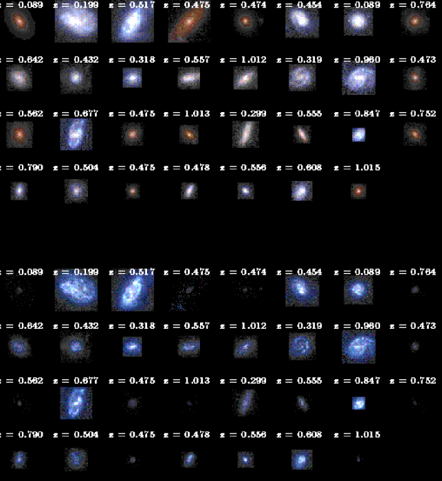
Figure 2: Colour images of our magnitude-limited ($I_{814,AB}<22.33$) redshift sample from the HDF generated from the $I_{814}$, $V_{606}$, and $B_{450}$ images determined by k-correcting each pixel to $z=0.5$ (panel (a)) and to $z=2.5$ (panel (b)). The intensity is scaled to the peak surface brightness to bring out the spatial detail at $z=0.5$ and to give a qualitative assessment of the importance of the k-correction for various portions of the galaxies, thereby illustrating the strong contrast between ellipticals and HII regions at high redshift. The ordering in this figure is by apparent magnitude with the brightest in the upper left-hand corner and the measured redshifts being listed for identification. For the sake of clarity, these images are not scaled or rebinned in area as in our simulations.

The resultant bright sample is listed in Table 1, along with our determination of its coordinates, $I_{814}$ magnitude, absolute magnitude, surface brightness (taken to be $m_{b_{J}^{0}}/(2\pi r_{hl}^{2})$), (where $m_{b_{J}}$ is the rest-frame $b_{J}$ apparent magnitude and $r_{hl}$ is the half-light radius), our eye-ball determination of the morphological type, and the known redshift. For reference we also include our determination of the k-correction over the surface of each galaxy at $z=2.5$. The calculation of k-corrections, rest-frame absolute magnitudes, and rest-frame surface brightnesses are described below. In addition, the redshift distribution of our bright subset is shown in Figure 1, for comparison with all of the redshifts measured in the compilation by Cohen et al. (1996), which includes the HDF and its flanking fields. We display the images of the bright sample in Figures 2a and Figure 2b, as a set of colour images ($B_{450}$, $V_{606}$, and $I_{814}$ bands) as they appear if k-corrected to the mean bright sample redshift, $z=0.5$, and also to $z=2.5$, using the pixel-by-pixel k-corrections described in the next section.

3 Representation of Each Sample Galaxy

3.1 The Light

We treat our bright galaxies as two-dimensional pixelated light-emitting surfaces for the purpose of k-correction, avoiding the unnecessary step of parameterizing their light profiles. We do not attempt to alter the inclination of each galaxy in the simulations, with the attendant problems regarding extinction this would entail, since by default our sample already contains galaxies of all orientations.

The question arises as to the best method of k-correction when the redshift extends to wavelengths short enough that no UV information is available. The spectrum of any given pixel is only sampled by 4 broad passbands and no information exists shortward of 2000 $\AA$ in the restframe of the typical bright galaxy (for which $\bar{z}\sim 0.5$), allowing a reliable k-correction to $z\sim 3$ in the longest wavelength band, $I_{814}$. In order to extend this work to higher redshift and in order to implement a smooth interpolation between the four passbands we adopt empirical template spectra. To indicate the robustness of the results to the choice of templates, we compare simulations for two independent sets of templates, one based on the small but large aperture UV sample of Coleman, Wu & Weedman (1980) and the other on the larger but small aperture sample of template spectra carefully compiled and combined from the IUE archive by Kinney et al. (1996). These data sets provide useful UV spectra for a range of optically selected galaxies nicely spanning the observed spectral range (see Connolly et al. 1996), so that a reasonable empirical interpolation and extrapolation can be performed by matching these templates to the 4 passbands of the HDF and improved by interpolating between these spectra to provide a smooth result. Additionally, we include the average effects of the HI Lyman continuum and series forest absorption at high redshift, as parameterized by Madau (1995) for distant QSO’s, since they significantly affect the broad-band colours of high redshift galaxies.

Formally, we represent each element $(\vec{x})$ in the two-dimensional template of a galaxy by

$$F_{\vec{x}}(\lambda)=\mu(\vec{x})f_{s(\vec{x})}(\lambda)$$ (1)

where $\mu(\vec{x})$ is the surface brightness template at element $\vec{x}$ in the $b$ band and where $f_{s(\vec{x})}(\lambda)$ is the spectral energy distribution shape at the element $\vec{x}$. We take the surface brightness template to equal that observed in the HDF in band $b$, the band with the highest integrated signal-to-noise (either the $I_{814}$ or the $V_{606}$ band for the objects in our sample.) For clarity we use the word “element” when referring to a pixel in the original bright galaxy image because these pixels are transformed in area and flux by redshift, and therefore distinct from the pixel scale of the simulations which is set by the HDF.

We take the SED shape, $f_{s(\vec{x})}(\lambda)$, for each element $\vec{x}$ from two different compilations of spectral templates: the Coleman, Wu, & Weedman (1980) (hereinafter, CWW) set supplemented with the NGC4449 spectrum (Bruzual & Ellis 1985, unpublished) and the Kinney et al. 1996 (K96) spectra. CWW includes SEDs intended to be representative of the dust-free E, Sbc, Scd, Sdm, and starburst (NGC4449) galaxies, and the K96 set includes SEDs intended to represent ellipticals, Sa, Sb, and SB1 (starburst; $E(B-V)\leq 0.3$) galaxies. We extend these observed SED templates below 1200 $\AA$ and 1400 $\AA$ respectively, by extrapolating the slope of the SED at these wavelengths down to the Lyman break at 912 $\AA$, below which we set the observed flux to zero (see Figure 3). We also interpolate linearly between spectra to form a smoothly continuous set for better fitting the observed 4 passband flux measurements.

Integrating the SEDs over the transmission curve of the 4 passbands, we then find the most-likely spectral template for each element $\vec{x}$, which we shall call $s(\vec{x})$, such that the sum of the squares of the differences between the SED template fluxes and the observed fluxes divided by the expected error in these fluxes is a minimum. The expected error is taken to be the error in the value of the pixel fluxes added in quadrature with the typical cosmic variance in the model SED fluxes ($0.^{m}25$) we find. Note that where the signal in a pixel is less than twice the sky noise, we have set the signal in that pixel equal to the value given by Eq. (1), adopting the surface brightness profile and the spectral energy template which best matches the mean value determined in a 1.0 arcsec diameter aperture. We have not attempted to realign the HDF images in the different bands, nor have we tried to correct for the different shapes that the PSF has in the different bands, since checks indicate that these effects are small and induce changes on scales smaller than the HDF pixel scale, i.e., 0.04 arcsec. This wavelength independence is due to the undersampling of images by WFPC, the effective HDF PSF being more set by the wavelength independent sub-sampling grid pattern than by the wavelength dependent diffraction of the telescope.

Clearly, we should take the spatial extent of each prototype image to be as large as possible within the limits of the signal. In practice, we take this to be the radius at which the mean pixel signal within an elliptical annulus is equal to the sky noise. Inspection of each image allows us to filter out the small number of obviously unrelated galaxies within this extended aperture, the pixels affected being replaced by their reflected counterparts. To be sure of including the “whole” object we extend its 2D profile by 50%, using the radial gradient. For this extended region we produce the noise by adding Poisson noise from modeled signal in quadrature with the general background noise. Except for the very brightest “cloned” galaxies, this extrapolation is not relevant, since the vast majority of replicated images generated from a given template galaxy are much fainter than the original, lying at higher redshift where these outer regions of the profile lie further into the noise.

The question arises as to the utility of the HDF $U_{300}$ images for generating the higher redshift images in the redder bands, since the sensitivity of the redder bands of the HDF is greater than that of the $U_{300}$ band. As it turns out, the signal in the HDF $U_{300}$ images is more than sufficient for our purposes, due to the strong $(1+z)^{4}$ cosmological surface brightness dimming. To see this, consider the S/N at a given $\sigma$ in a pixel through the $U_{300}$ filter at the observed redshift. This translates into a lower S/N at higher redshift in the other bands, given their relative sensitivities and exposure times. Taking the worst case that the spectrum of a given pixel is flat in frequency (though in practice the spectral indices of some starburst systems are somewhat steeper than this), the surface brightness dims by a factor $7.5\log\frac{(1+z)}{(1+z_{obs})}$, or $7.5\log\frac{\bar{\lambda_{b}}}{\bar{\lambda_{F300W}}}$, or a decrease of the surface brightness by 1.3, 2.3, and 3.3 $\textrm{magnitudes/pixel}^{2}$, for the $B_{450}$, $V_{606}$ and $I_{814}$ bands respectively. However, the measured 1-$\sigma$ $U_{300}$ noise level for the HDF is 32.4 $\textrm{mag/pixel}^{2}$, compared to the 32.2, 34.0, and 32.6 $\textrm{mag/pixel}^{2}$ levels in the $B_{450}$, $V_{606}$, $I_{814}$ bands. Clearly, then, since few pixels are as blue or bluer than a flat spectrum in our template galaxy sample, the S/N of any pixel in a redder band at higher redshift will always be less than that of the observed $U_{300}$ image.

While it is apparent that a number of objects in our input sample have extremely low values of S/N in the $U_{300}$ band (see the ellipticals in Figure 2a), we emphasize that the S/N in $U_{300}$ is always sufficient to determine the appearance of these galaxies at higher redshifts in the redder bands of the HDF given the relative band sensitivities and exposure times used in these passbands. Greater inequities between bands would limit the simulations to depths less than the limiting magnitudes of these passbands.

3.2 Space Density

We set the space density of each galaxy in our sample equal to ${1/V_{max}}$, determined by the maximum redshift, $z_{max}$, to which each galaxy could have potentially been selected given our chosen magnitude limit. $V_{max}$ is given by

$$V_{max}=S\int_{0}^{z_{max}}\left(\frac{d_{L}}{1+z}\right)^{2}\frac{cdz}{H_{0}E(z)}$$ (2)

where

$$E(z)=\sqrt{\Omega(1+z)^{3}+(1-\Omega-\Omega_{\Lambda})(1+z)^{2}+\Omega_{\Lambda}}$$ (3)

where $S$ is the solid angle of the surveyed area and where $d_{L}(z_{max})$ is the well-known luminosity distance at redshift $z_{max}$. $z_{max}$ is determined by:

$$22.33=I_{814,AB}+k_{814}(z_{max})-k_{814}(z_{obs})+5\log\frac{d_{L}(z_{max})}{d_{L}(z_{obs})}$$ (4)

where $z_{obs}$ is the observed redshift and $k_{814}(z)$ is the $k$-correction in the $I_{814}$ band at redshift $z$. We determine the $k$-correction for the galaxy from the total spectral energy distribution, which incorporates the contribution of all the elements in our two-dimensional representation of each galaxy. Note this procedure avoids the usual steps of constructing a luminosity function, parameterizing it, and then assigning k-corrections. We simply treat each galaxy as a class of its own with a space density set by its own value of $1/V_{max}$, allowing a fully unbinned, individual treatment of each template galaxy.

4 Consistency Checks and Sample Fairness

Astronomers have long used the $V/V_{max}$ distribution (Schmidt 1968) to assess the completeness and uniformity of a sample, where $V$ is the volume up to and including the redshift of the galaxy in question and $V_{max}$ is the volume in which this galaxy could have been observed, given the selection criteria. For a uniform distribution of galaxies in a volume one expects a uniform distribution of $V/V_{max}$ between 0 and 1, in the absence of evolution and clustering, and for a sample with $N$ galaxies the average value of this quantity us given by:

$$\left\langle\frac{V}{V_{max}}\right\rangle=0.5\pm\frac{1}{\sqrt{12N}}$$ (5)

The distribution of $V/V_{max}$ for our template sample is shown in Figure 4, for $\Omega=0.1$/$\Lambda=0.9$, $\Omega=0.1$, and $\Omega=1.0$, where the k-correction is formed from the SED averaged over the whole object. The average value for the $V/V_{max}$ distribution is 0.48, 0.51, and 0.53 for the $\Omega=0.1$/$\Lambda=0.9$, $\Omega=0.1$, and $\Omega=1$ geometries, which is within the expected deviations for the $V/V_{max}$ statistic $(0.50\pm 0.05)$ and not inconsistent with the rate of evolution detected in a larger redshift survey to a similar magnitude limit (Lilly et al. 1995). We could have chosen to derive $V_{max}$ by redshifting each pixel of the object and performing the photometry on the redshifted image for greater self consistency, but this turns out to be virtually irrelevant because the magnitudes we recover from the redshifted images placed at $z_{max}$ are on average displaced by only 0.07 magnitudes faintward of our magnitude limit ($I_{814,AB}=22.33$). A slight faintward shift is expected for aperture magnitudes since the lower surface brightnesses at $z_{max}$ results in some small loss of the light on the wings. To illustrate this point, we compare the recovered magnitudes at $z_{max}$ with the magnitude limit chosen for our bright sample in Figure 5.

To provide a basic context for understanding the no-evolution simulations described above we display the luminosity function obtained for this sample in Figure 6, for two different representative cosmologies. We compare this luminosity function with the $b_{j}$-band luminosity functions determined by Loveday et al. (1992) and Zucca et al. (1997) in the APM and ESP surveys, respectively correcting our sample to restframe $b_{j}$ directly using our pixel-by-pixel best-fit SEDs. We see that our luminosity function is shifted to larger luminosity and/or space density than that of the local universe, broadly consistent with the findings of Ellis et al. (1996) and Lilly et al. (1995) where the luminosity function of blue objects is observed both to brighten and to steepen.

We can also compare our sample with the redshift distribution, N(z), of the Canada-France Redshift Survey (CFRS), a survey of similar depth, by simulating (as described in detail below) its survey parameters. The CFRS sample covers $17.5<I_{AB}<22.5$ over 112 $\textrm{arcmin}^{2}$. Scaling by these criteria and the 19% redshift incompleteness of the CFRS, we can construct a prediction for N(z) using our method (Figure 7). We make a small correction, inferable from Figure 5 of Lilly et al. (1995), to convert from isophotal to total magnitudes by a uniform 0.1 mag. A noticeable difference between our predicted N(z) and that of the CFRS is found in the amplitude of the distributions, our redshift distribution being 28% higher, consistent with the differences in the respective luminosity functions (Figure 6). Despite this, the shape of our predicted N(z) is very similar to that of the CFRS, which is not surprising given the wide spread of $V/V_{max}$ for our sample (Figure 4). This basic agreement is quite satisfactory, showing that our bright galaxy sample fairly samples the range, if not quite the average density, of galaxies comprising the general field population.

5 HDF Simulations

According to the number density derived for each template galaxy, $1/V_{max}$, and assuming homogeneity, we generate Monte-Carlo catalogues of the objects out to very large redshift ($z=7$) over the solid angle of the HDF, each object being assigned a random redshift, position, and position angle. We then generate mock images on the basis of these catalogues. Each redshifted image must be scaled in size and resampled with more noise and additional PSF smoothing to account for its higher redshift and generally smaller size relative to its brighter counterpart. Since the two-dimensional surface brightness profiles of the bright galaxies already contain noise, we find it useful to simultaneously generate both a signal $I$ and noise $N$ image. The noise image $N$ keeps track of how much noise has been implicitly added to each pixel in the signal image $S$ by virtue of each galaxy template implicitly containing noise. Such an accounting allows the proper amount of noise to be added to each pixel in the signal image after all the scaled galaxy templates have been laid down.

To generate an image at a chosen redshift, we must calculate the change in size and surface brightness of each element $\vec{x}$ in our two-dimensional galaxy templates. For a galaxy with redshift, $z$, we take the angular size of each element in our two-dimensional galaxy template, $d_{z}$, to be equal to

$$d_{z}=\left(\frac{d_{A}(z_{obs})}{d_{A}(z)}\right)d_{gal}$$ (6)

where $z_{obs}$ is the redshift of the object as measured in the HDF, $d_{A}$ is the angular distance (Peebles 1993), and $d_{gal}$ is the angular size of each element in our two-dimensional galaxy template image at $z_{obs}$, i.e. the pixel size of galaxies in the HDF (0.04 arcsec). We calculate the surface brightness $\mu^{X}(\vec{x},z)$ that each element $\vec{x}$ of our two-dimensional galaxy template has at redshift $z$ for a given passband $X$ as

$$\mu^{X}(\vec{x},z)=\mu(\vec{x})+k^{X}(\vec{x},z)-k^{b}(\vec{x},z_{obs})+2.5\log\left(\frac{1+z}{1+z_{obs}}\right)^{4}+(X-b)(\vec{x})$$ (7)

where $k^{b}(\vec{x},z)$ and $(X-b)(\vec{x})$ are the $k$-corrections and $z=0$ $X-b$ colours calculated based on the spectral energy distribution $f_{s(\vec{x})}$ of element $\vec{x}$. We have included the line blanketing by the Lyman-alpha forest as given by Madau (1995) as well as Lyman-limit absorption in our calculations of the $k$-corrections since these corrections become important at $z>2.0$ in the $U_{300}$ band and at $z>3.5$ in the $B_{450}$ band.

In calculating both the signal and the noise at each pixel on the images $I$ and $N$, we break up each pixel into 25 smaller subpixels, and calculate the contribution of each redshifted element $\vec{x}$ to each of these smaller subpixels to account for the generally much larger area covered by a data pixel than that of the redshifted image element, for the purpose of rebinning.

Because the real PSF has smoothed each galaxy template, to correctly calculate the appearance of each prototype galaxy in our sample at higher redshifts we must add more smoothing present in each object in the $I$ image, depending on the reduction in angular size for the object in question. For simplicity, we simply smooth each object with a kernel derived from a relatively isolated, unsaturated star from the Hubble Deep Field reduced in size so that its scale length is simply $\sqrt{1-\left(\frac{d_{A}(z_{obs})}{d_{A}(z)}\right)^{2}}$ times that of the original scale length. The above expression is exact for the case of a perfectly Gaussian PSF and is also close to exact in those cases where the angular size of the simulated galaxy laid down in the $I$ image is much smaller than the HDF. Of course, it is true that the real HDF PSF differs from a Gaussian in that it has much more extended wings, but for the most part the differences that this makes are small. To verify this, we compared the angular sizes recovered using the present procedure and from assuming the PSF to be exactly Gaussian (the $\sigma$’s for which we determined by fitting to the same unsaturated star in the HDF), and we found little if any dependence on these differences.

For a pixel in which the contribution to the signal image $I$ from an element in the template image is $I(\vec{x})f$, the noise contribution to the same pixel in the noise image $N$ is taken to be

$$\frac{I(\vec{x})f}{(\frac{S}{N})(\vec{x})}\sqrt{\frac{d_{z}}{d_{gal}}}$$ (8)

added in quadrature, where $(\frac{S}{N})(\vec{x})$ is the S/N ratio calculated for the element $\vec{x}$ for the $\mu(\vec{x})$ template drawn from the HDF, and account is made of both the background and Poissonian noise associated with the measured pixel-by-pixel signal.

Having generated the signal image, we want to calculate the appropriate noise for each pixel in our simulated HDF, which we take to be:

$$N(\vec{x})_{desired}=\sqrt{\sigma^{2}+(I(\vec{x}))^{2}G}$$ (9)

where $\sigma$ is the background noise level in the HDF, $I(\vec{x})$ is the signal at pixel $\vec{x}$, and $G$ is the gain.

Having already calculated the amount of noise which each pixel in the signal image had by virtue of implicit noise in the templates, i.e. the noise image $N$, we can bring the noise in each pixel up to the appropriate value $N_{desired}$ by adding pixel-by-pixel Gaussian-distributed noise with standard deviation $\sqrt{N_{desired}^{2}-N^{2}}$, smoothing this added noise with the noise kernel specified in Table 4 of Williams et al. (1996) so as to approximate the observed correlation properties of the noise in the HDF. While the outlined procedure will add the appropriate amount of noise to pixels if noise is lacking in those pixels, it is possible that some pixels will already have more noise added to them than is present per pixel in the HDF. In particular, this occurs when the redshift for an object is lower than that of the prototype, since of course we cannot improve on the S/N of the prototype galaxy image. To artificially prevent this possibility, we simply replace every galaxy in our mock catalogue whose redshift is lower than its observed redshift, with another galaxy from our bright sample placed at the same redshift whose observed redshift is lower than the mock catalogue redshift. Though this results in a bright galaxy population which is slightly unrepresentative (and, in fact, this is the cause of the slight disagreement observed in the distribution of bright HDF galaxies and the simulations found later in the paper), it does not appreciably bias the measured properties of the cloned galaxies at the fainter magnitudes of interest.

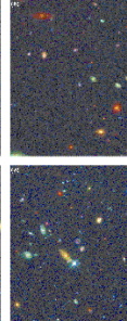
Figure 8: Panels (a), (b), and (c) show 52” x 72” colour images generated from our no-evolution simulations for the $\Omega=1.0$, $\Omega=0.1$, and $\Lambda=0.9$/$\Omega=0.1$ geometries, respectively, of the $B_{450}$, $V_{606}$, and $I_{814}$ images, constructed with pixel size, S/N, and PSF identical to that of the HDF. Panel (d) shows an image of the same size taken from the HDF. Clearly, the no-evolution simulation strongly underpredicts the total number of faint galaxies in the HDF.

The simulations cover a sky area four times that of the HDF in each of the four broadbands $U_{300}$, $B_{450}$, $V_{606}$, and $I_{814}$. We perform these simulations self-consistently for $\Omega=0.1$/$\Lambda=0.9$, $\Omega=0.1$, and $\Omega=1$, by which we mean that the $V_{max}$ of the bright sample uses the same geometry as the volume used in constructing the simulation. In Figure 8 we compare a no-evolution simulation assuming $\Omega=1.0$, $\Omega=0.1$, and $\Lambda=0.9$/$\Omega=0.1$ with an area of the same size selected from the HDF.

A simple test of our procedure is to construct images of the 31 prototype galaxies at their observed redshifts ($z_{obs}$). Good agreement is found between these images and their originals at $z_{obs}$, within the errors expected on the basis of our pixel-by-pixel SED fits. To illustrate this agreement more quantitatively, we plot a comparison of the recovered values for the half-light radius, Petrosian radius (Petrosian 1976), and apparent $I_{814}$ magnitudes in Figure 9.

6 Object Detection

On both the simulations and the HDF itself, we perform the object identification and photometry using SExtractor version 1.2b5 (Bertin & Arnouts 1996). After smoothing the $I_{814}$ images with a Gaussian of 0.06-arcsec radius (the approximate PSF) within SExtractor, we require that objects be at least 2 sigma above the noise over an area of at least 10 contiguous pixels, and we use a cleaning parameter of 1.0. We select our apparent magnitudes to be equal to SExtractor’s $MAG\_BEST$ estimate, which for non-crowded objects is equivalent to an isophotal magnitude extrapolated beyond the isophotes. We exclude objects with half-light radii less than 0.15 arcsec and $I_{814,AB}<23$ as stars, fainter than which the contamination is relatively small. Then, based upon the detected objects, we used SExtractor to determine the apparent magnitudes in the other bands with the $I_{814}$ apertures.

We set the deblending parameter ($DEBLEND\_MINCONT$), which is important in determining the extent to which SExtractor breaks up objects, to be equal to 0.04. We found some dependence of our results on the value chosen for this parameter, particularly the break-up rate, but for the most part this dependence was small. Our chosen value of the deblending parameter is very close to that (0.05) used by Clements & Couch (1997) (Couch, private communication). With this choice of parameter, we obtained the reasonable result that no bright galaxy from our sample broke up into smaller pieces when placed at its $z_{max}$, in agreement with our qualitative impressions in looking at these images.

We derive two different measures of the angular size for each object in our image, a Petrosian radius (Petrosian 1976) and a half-light radius. We take the Petrosian radius to equal the smallest radius for which the surface brightness at that radius equals half the average surface brightness interior to that radius. The half-light radius is equal to the radius of the aperture which contained half the light as determined by SExtractor’s best estimate of the total light. We performed some simulations to test our method for recovering half-light radii and found that our recovered half-light radii are only slightly scattered about sizes 10% smaller than the input half-light radii at $I_{814,AB}\sim 24$. The scatter in this relationship partially derives from the uncertainty in the overall photometry performed by SExtractor.

7 Results

7.1 Number Counts in the $I_{814}$ band

It is natural to begin our comparison of the faint galaxy population in the HDF by looking at the counts in $I_{814}$, the longest wavelength band and hence least affected by uncertainty in the k-correction. Figure 10 compares the number counts recovered from both our simulations and the observations (a description of the plotted $1\sigma$ estimates based on the size of our bright sample is given in Appendix A.) For all geometries, we find that our no-evolution predictions fall steadily short of the observations with increasing apparent magnitude. For $\Lambda=0.9$/$\Omega=0.1$, the shortfall is noticeably less pronounced due to the relatively larger volume available. At $I_{814,AB}=26$, for example, the counts fall short by a factor $1.9\pm 0.4$ for $\Lambda=0.9$/$\Omega=0.1$ compared to $5.4\pm 1.0$ for $\Omega=1$ and $2.7\pm 0.8$ for $\Omega=0.1$.

Of course, the counts recovered at bright magnitudes, $I_{814,AB}\approx 22$, are in fair agreement with the observations, as one would expect given the definition of our sample up to approximately the same bright limit, $I_{814,AB}=22.33$. It is reassuring to find that there little dependence of the number counts on the choice of spectral template, whether it be the CWW set or the K96 set. Finally, as discussed in Appendix B, we note that the present no-evolution faint counts ($I_{814,AB}\sim 28$) are compromised of a non-negligible number of the input prototype galaxies ($\gtrsim 10$).

7.2 Number-Count Completeness, Overcounting, and Clustering

Given our knowledge of the positions, redshifts, magnitudes, and types of galaxies laid down in each simulated image, it is simple to determine systematic uncertainties such as incompleteness in the number counts, by matching up the object catalogues from the simulations created by SExtractor with our input Monte-Carlo catalogues. Figure 11 shows that the incompleteness becomes significant in the range $I_{814,AB}>26$ for both our no-evolution simulations. This incompleteness stems from the fact that at fainter magnitudes, we are sensitive to smaller and hence the higher surface brightness galaxies, so that large fraction of the population of galaxies at faint magnitudes subtend areas too large for detection given their redshifted surface brightnesses.

In a similar manner, we can determine the rate of overcounting of in our simulated fields. As explained in Colley et al. (1997), it is possible to overcount the number of faint galaxies by misidentifying individual parts of a galaxy as distinct galaxies, especially at higher redshifts, where the rest-frame ultraviolet light is accessed and HII regions have a higher contrast (cf. the galaxy at $z=0.319$ in Figure 2b). For simplicity, rather than perform an angular correlation analysis like Colley et al. (1997), we have chosen to measure this number directly. In Figure 12, we display the rate of overcounting for all the simulations performed by comparison of the input random catalogue with those recovered. Clearly, in our no-evolution simulations, using the parameters chosen for the photometry, overcounting is never an important effect for any of the cosmologies examined.

The clustering seen in the HDF redshift data at bright magnitudes (Figure 1) is responsible for the overdensity at bright magnitudes $I_{814}<22.33$ in the HDF relative to the mean field counts measured in wider field surveys. Compared to the CFRS, for example, this amounts to a $\sim 28\%$ overdensity (Figure 7). At fainter magnitudes, however, the count variance should be less affected by clustering, given the greater projected volume and the expectation of less well developed structure at earlier times. We provide a quick test of the plausibility of this hypothesis using other deep HST $I_{814}$ data. Figure 13 shows the count variance between 6 pointings (two sets of 3 HST pointings separated by 3 hours on the sky from another program). These data show that the count variance in $I_{814}$ band decreases steadily to the Poissonian limit ($I>25$) over the area of WFPC2, consistent with isotropy at faint magnitudes.

7.3 Angular Sizes

We compare the distributions of half-light radii recovered from the HDF with those of our “no-evolution” simulations in Figure 14. The hatched area represents the $1\sigma$ uncertainty range based on the finite size of our bright sample for the no-evolution model using the CWW SED templates. The solid curve indicates the angular size distribution recovered from simulations using the K96 SED templates. At bright magnitudes ($21<I_{814,AB}<22.6$), the angular sizes recovered from the simulations agree quite well with the observations as expected given the fact that we defined our bright sample in terms of many of these same galaxies.

In contrast, at fainter magnitudes, the half-light radii from the no-evolution simulations become significantly larger than those from the observations: larger by 43%, 44%, and 57% in the magnitude range $24<I_{814,AB}<26$ and larger by 35%, 42%, and 53% in the magnitude range $26<I_{814,AB}<27.5$ for the $\Lambda=0.1$/$\Omega=0.1$, $\Omega=0.1$, and $\Omega=1$ geometries, respectively, where the median of the angular size distribution in each magnitude bin is used for comparison. As expected, we see that galaxies in the $\Lambda=0.9$/ $\Omega=0.1$ geometry tend to possess smaller angular sizes than galaxies in the $\Omega=0.1$ geometry and especially galaxies in the $\Omega=1.0$ geometry because of the somewhat larger angular-diameter distances.

We repeat the above comparisons using the Petrosian radii instead of the half-light radii. Ideally, Petrosian radii provide a more reliable surface brightness-independent estimator of the angular size than half-light radii, though one might question its meaningfulness given the increasingly lumpy appearance and small sizes of faint galaxies. In any case, an inspection of Figure 15 shows that the same general trends and conclusions hold here as for the half-light radii.

7.4 Colour Distributions

In Figure 16-17, we plot a comparison between the colour distributions recovered from the observations and our ‘no-evolution’ simulations in three different magnitude ranges for two different colours, $(B_{450}-I_{814})_{AB}$ and $(V_{606}-I_{814})_{AB}$. Good agreement is found at the bright magnitudes ($21<I_{814,AB}<22.6$) as expected given that our bright sample is selected up to this magnitude limit. At fainter magnitudes, however, a clear excess of bluer galaxies is observed relative to our no-evolution simulations. In addition, in the faintest magnitude bin ($26<I_{814,AB}<27.5$), there also appears to be an excess of red galaxies relative to that found in the no-evolution simulations. This is somewhat unexpected because one would expect the real universe, for which our sample is representative at $z\sim 0.5$ to have a younger and therefore bluer appearance than that of our extrapolated sample. This excess may, therefore, reflect the presence of dust and Lyman-series forest absorption at moderate to high-redshift. Conceivably, an ad-hoc maximal dwarf-model, might also account for this red excess in terms of faded dwarfs at low redshift.

7.5 Redshift Distributions

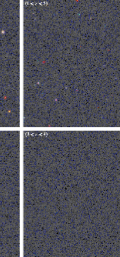
Figure 19: Simulated 52” x 72” colour images generated from the $B_{450}$, $V_{606}$, and $I_{814}$ bands for four different redshift slices ($0<z<1$, $1<z<2$, $2<z<3$, and $3<z<4$) using a $\Omega=0.1$ no-evolution simulation with pixel size, signal-to-noise, and PSF identical to that of the HDF. Note the decreased visibility of our bright galaxy sample at high redshift.

In Figure 18, we plot the redshift distributions of the galaxies recovered by SExtractor by matching them up with our input catalogues. It is apparent that in the absence of evolution very few galaxies lie beyond a redshift $z=2$, even at the faintest magnitude, with little dependence on the choice of geometry. A dramatic illustration of the relative unobservability of high redshift galaxies for $\Omega=0.1$ is given in Figure 19, where we have broken up the simulation of a 52” x 72” HDF exposure into 4 redshift slices.

It is interesting to see how these distributions compare with the photometric redshift estimates derived from fits to the 4 passbands of the HDF, and from subsequent near-IR imaging of this field from the ground. Surprisingly enough, the redshift distribution recovered from our “no-evolution” simulations agree remarkably well with the approximate distribution of Lanzetta, Yahil, & Fernandez-Soto (1996). Given that similar coincidences have been found for redshift surveys at somewhat brighter magnitude limits (Broadhurst et al. 1988; Colless et al. 1993; Cowie et al. 1996), it is somewhat tempting to suppose that this result might hold to yet fainter magnitudes. Despite such hopes, clearly this relationship begins to break down in the $B$ band at fainter magnitudes ($B>24$), at least, as Cowie et al. (1996) have shown, and presumably a similar break down will occur in the redder bands at fainter magnitudes.

7.6 $U_{300}$ and $B_{450}$ “Dropouts”

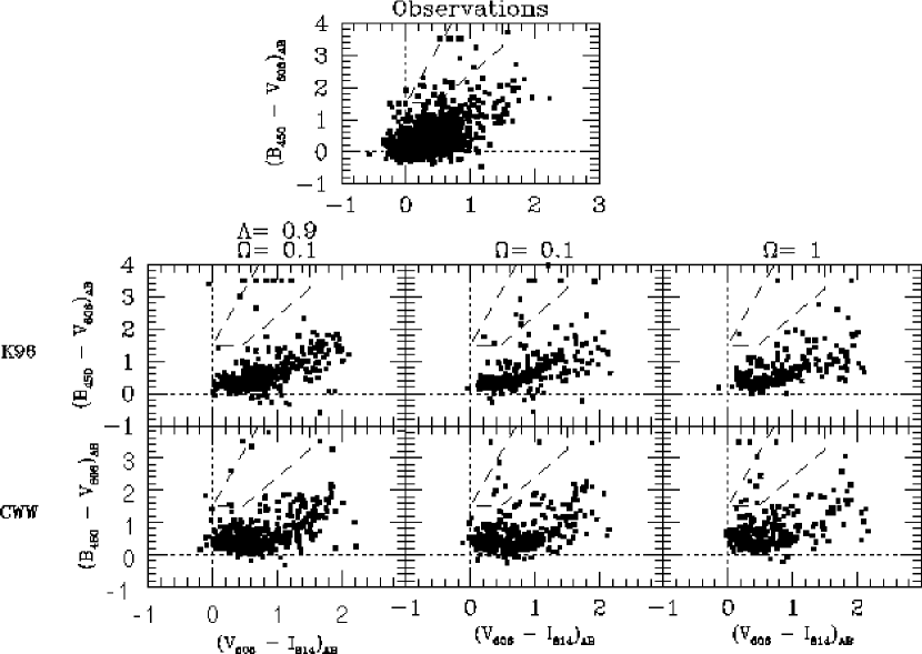
Figure 21: Comparison of the $(B_{450}-V_{606})_{AB}$ versus $(V_{606}-I_{814})_{AB}$ diagrams for our no-evolution simulations with the CWW SED templates (lowest panel) and our no-evolution simulations with K96 SED templates (top panel) against the observations for galaxies with $V_{606,AB}<28.0$ (the same criterion used in Madau et al. 1996). With a dashed line, we have overplotted the $B$-band dropout region suggested by Madau et al. (1996) for finding high redshift ($3.5<z<4.5$) galaxies whose Lyman-limit crosses the $B$ bandpass. Note that galaxies near the top of the colour-colour diagram, i.e., with $(B_{450}-V_{606})_{AB}>3.5$, are simply lower limits on the $(B_{450}-V_{606})_{AB}$ colour. As with the $U_{300}$ dropouts, these no-evolution simulations underpredict the number of dropouts.

In Figures 20 and 21, we plot several colour-colour diagrams, and overplot the $U_{300}$-dropout and $B_{450}$-dropout selection criteria given by Madau et al. (1996), criteria, useful for selecting galaxies at redshifts $2<z<3.5$ and $3.5<z<4.5$, respectively. We count the number of recovered galaxies satisfying these criteria and provide a sumary in Table 2. As expected from the recovered redshift distributions plotted in Figure 18, it is clear that the no-evolution simulations contain manifestly fewer dropouts than the observations. Clearly then, the high-redshift universe contains a larger number of objects which of greater luminosity in the ultraviolet than the galaxy population in our redshift-complete sample.

We have compared the numbers of dropouts in the HDF found by Madau et al. (1996) with our values listed in Table 2, using the same colour-magnitude window. Our dropout rate is higher for the HDF, a finding which might result from our use of SExtractor for photometry rather than FOCAS as employed by Madau et al. (1996). Given that these programs likely differ with regard to the degree to which they successfully estimate the magnitudes of detected objects, our analyses probably probe slightly different depths, even though we choose for comparison the same nominal magnitude limit ($I_{814}<26.79$). Imposing a magnitude limit $0.^{m}3$ brighter, we can reproduce their dropout rate. Also, as stated by Madau et al. (1996), their FOCAS magnitudes are in general estimated to be too faint by about $0.^{m}5$.

7.7 Asymmetry

In the light of recent work attempting to quantify the morphology of faint galaxies, we compare the properties of the faint galaxies from the HDF against those from our simulations with the $A$ statistic proposed by Abraham et al. (1996a,1996b), in order to provide an approximate estimate of the extent to which evolution may affect the asymmetry of galaxies, where $A$ is defined as the sum of the absolute value of the differences between a galaxy image and itself rotated 180 degrees about the center of the image. The approximate contribution of the noise to the apparent asymmetry is calculated and subtracted. We plot the distribution of this asymmetry parameter recovered both from our simulations and from the HDF in Figure 22, for two different magnitude bins. We find a clear trend toward larger values of this parameter with increasing magnitude. At the simplest level, this would seem to imply that the faint galaxies are less smooth than the redshifted field population at $z\sim 0.5$ used in our simulations.

Some caution must be exercised in interpreting the $A$ statistic since it appears to be extremely sensitive to the manner in which one determines the center about which to rotate for evaluating the statistic (Abraham & Brinchmann, private communication) and can exhibit a fair amount of scatter ($\pm 0.1$) depending upon whether one takes the centroid or the maximum as the for the center. Because of this, the statistic, or at least the present implementation, seems to become increasingly unreliable for the smallest galaxies and hence we restrict our comparison to the bright magnitudes ($I_{814,AB}<26$) where we are more confident in the reliability of the statistic from our own internal tests.

Note that along similar lines, based upon pixel-by-pixel k-corrections of the Frei, Guhathakurta, & Gunn (1996) sample and systematic applications of asymmetry ($A$) & central-concentration ($C$) statistics, Abraham et al. (1996a,1996b) have argued that the fainter galaxy population is quite unlike the local galaxy population broadly represented by the Frei et al. (1996) sample, which is nevertheless somewhat ill-defined, lacking a firm magnitude limit or well-defined selection criteria.

8 Discussion

Since the novelty of the HDF is principally its angular size information obtained to unprecedentedly faint magnitudes, it is not too surprising that our most interesting finding relates to the sizes of the faint images. The count excess is clearly composed of galaxies with smaller projected areas than expected on the basis of relatively low-redshift galaxies ($\bar{z}=0.5$) for any interesting geometry. The evolution of angular-size has not been completely clear in the literature to date. Previously, in the range $24<I<25$, Roche et al. (1996) find an apparent excess of galaxies with small angular sizes relative to their no-evolution models which are designed to replicate the angular sizes of galaxies in the local universe. At brighter magnitudes ($I\approx 22$), the study by Im et al. (1995) on the prerefurbished HST data indicates that the angular sizes of this population is also smaller than expected based upon more local, brighter measures. However, there have also been some studies based on this parallel data indicating no changes in size (Mutz et al. 1994; Casertano et al. 1995).

We also find that the number density of dropouts discovered at faint magnitudes exceeds that recovered from our no-evolution simulation, a finding which clearly indicates that the real high-redshift universe contains a larger density of galaxies with high UV surface brightnesses. Note, however, that despite this finding, the estimated integrated star-formation rates in these redshift ranges are similar (Madau et al. 1996). Clearly, then, as argued in Steidel et al. (1996) and Lowenthal et al. (1997) (cf. Figure 7), more star-formation took place on relatively small scales at high-redshift. It remains unclear whether this is the result of the intrinsically smaller baryonic aggregations or the increasing prominence of starbursts at high redshifts.

Our finding that overcounting rates do not seem to be very important (see also the companion paper: Bouwens, Broadhurst, & Silk 1998) is somewhat contrary to the claims of Colley et al. (1997), even though we used a similar program (SExtractor) with similar values of the deblending parameter as one catalogue (Clements & Couch 1997) used in their study. Of course, the galaxy population we have used for our study is more evolved than expected in the real universe at higher redshifts, so we might expect our value to be an underestimate. Note that in any case, the small scale correlation claimed is a statistically marginal result, ($\sim 1.5\sigma$, Colley et al 1997).

Less contentious are our findings regarding the colours and the number counts. In agreement with most authors we find clear evidence that the predictions without evolution are redder than observed (Lilly et al. 1995) and that the number counts fall short of the data at faint magnitudes (Lilly 1993; Pozzetti et al. 1996).

As we have already argued, it is possible to see the present work as a demonstration that the trends found in comparing the local ($z\sim 0$) population with intermediate-redshift galaxies ($z\sim 0.5$) extend to yet fainter magnitudes and presumably higher redshifts. At these intermediate magnitudes a larger number of faint, blue, irregular, and presumably small galaxies (Ellis et al. 1996; Lilly et al. 1995; Brinchmann et al. 1998; Guzman et al. 1997) have been reported at $z\sim 0.5-0.8$ relative to local expectations. The present study demonstrates that the these trends extend to yet fainter magnitudes, in that there continues to be both an increase in the number and apparent starburst activity of the faint galaxy population as well as a decrease in mean galaxy size.

Uncertainty estimates for the present study are somewhat “internal” and, therefore, might underestimate a field-averaged variance in our measurements. Certainly, at bright magnitudes the HDF is $\sim 28\%$ overdense with respect to the CFRS. However, since 90% of our bright galaxy sample ranges over a wide spread in distance, some 1500 Mpc/h, and $V/V_{max}$ is evenly spread over the interval [0,1], most bright galaxies should be considered as independent. Clearly, we would prefer a larger, more local sample of redshift-complete bright galaxies for our simulations, and other deep multicolour HDF imaging would be useful in the first two respects.

9 Summary

We have developed a technique for generating a model-independent faint galaxy population based on pixel-by-pixel k-corrected images of the bright galaxy population, for comparison with deep high-resolution images. Our technique has the virtue of being model-independent and completely empirical, except for the usual choice of geometry. We have made use of the HDF for the purposes of defining a redshift-complete bright galaxy sample from which to construct empirical simulations and also for evaluating the evolution of the much fainter galaxies detected in the HDF. We have made use of all four passbands and have been able to make concrete statements about the evolution of the image properties with estimated uncertainties based on the size of a volume-limited sample. We find that, relative to our simulations based on the bright galaxy sample, the faint galaxies are smaller, more numerous, bluer, less regular, and contain more dropouts for any interesting geometry. Of particular note is our finding with regard to angular sizes, for which a variety of nebulous and seemingly contradictory statements may be found in the literature.

Our bright galaxy sample is small, and it will be important to see if our conclusions remain valid when a larger sample is available. Nonetheless, we believe this work is an important foundation on which to build, in particular, as we look forward to independent deep fields and the very significant improvement in the quality of UV and optical imaging promised by the Advanced Camera (Ford et al. 1996).

Appendix A Determination of Random Errors

Here we quantify the empirical model uncertainties due to the finite size of our input sample. We look at this uncertainty in terms of an arbitrary quantity describing the surface density of objects on the sky satisfying some observational criteria.

For any faint sample of objects satisfying a certain set of observable criteria ($S_{O}$), it is possible to express the probability distribution for the number of these objects as the sum of the probability distributions for this variable over all possible galaxy morphologies, luminosities, and sizes, i.e., $\sum_{i=1}^{N}f_{i}$. We suppose that this faint sample of galaxies is derived in a Monte-Carlo manner from our bright sample on the basis of no-evolution assumptions, so that it is possible to express this probability distribution for each galaxy type as the product of the probability distribution for the number of times this object will appear in our bright sample, call it $B_{i}$, and the probability distribution for the number of times such a galaxy would be expected to appear in the faint sample in question ($S_{O}$), call it $D_{i}$. In this way, the overall probability distribution for the number of galaxies observed in a given faint sample ($S_{O}$) can be expressed as

$$\sum_{i=1}^{N}B_{i}D_{i}$$

We shall suppose that each galaxy in our bright sample is sufficiently unique to be represented by its own term in the above equation. Furthermore, since each of these galaxies appeared in our bright sample once and only once, we suppose that $B_{i}$ is Poisson-distributed with a mean of 1, which we approximate as a normal distribution about this mean. For lack of something better, we shall take the probability distributions $B_{i}$ for all other galaxy types to be delta functions at 0.

Now, it is possible to estimate the uncertainty in the expectation value for the number of galaxies in our faint sample based on the finite number of galaxies we have in our bright sample. Because our simulated area is, in principle, unlimited, the uncertainty in the expectation value of $D_{i}$ is vanishingly small, and in practice we take this uncertainty to be zero. As such, the above probability distribution is simply the sum of normal distributions with various weights, and therefore its 1-sigma uncertainty is simply equal to $\sqrt{\sum_{i=1}^{N}D_{i}^{2}}$. We have used this expression throughout our paper in the estimation of errors for each observable calculated from our no-evolution simulations.

Appendix B Breakdown of Faint Samples

At fainter magnitudes, one expects a smaller number of the galaxy prototypes to make up an increasing fraction of our faint galaxy sample, as a result both of the differential k-corrections and of the relatively greater volume available to lower luminosity objects at fainter magnitudes. To quantify the importance of this trend, we compute a weighted measure of the effective number of galaxies which contribute to the counts in each magnitude bin, a quantity we take to equal

$$\left(\frac{\sum_{i=1}^{N}n_{i}}{\sqrt{\sum_{i=1}^{N}n_{i}^{2}}}\right)^{2}$$

where $n_{i}$ is the number of galaxies of a given prototype per magnitude per square degree recovered from our simulations and $N$ is the number of prototypes considered (i.e. 31). Basically, the above expression equals the square of the number counts divided by the estimated Poissonian error based on the size of the contributing sample at the magnitude in question, the derivation of which is given in Appendix A. In the case that all the $n_{i}$’s are the same, the expression reduces to $N$ as required.

We compute the above expression from our simulations, and we plot the results in Figure 23. At bright magnitudes, the bright galaxy catalogues are still dominated by shot noise so that the number of galaxies estimated from the above expression to contribute at any magnitude is lower than the real number ($\sim 31$) which contribute. At fainter magnitudes, the effective of number of galaxies decreases again for the reasons stated above, i.e., a relatively smaller differential volume for the more luminous galaxies and the k-correction. For the sake of clarity, we emphasize that at each magnitude, every galaxy prototype contributes some fraction to the number counts there.

Figure 1: Redshift distribution of our magnitude-limited sample ($I_{814,AB}<22.33$) from the HDF follow-up redshift surveys (solid histogram) plotted along with the redshift distribution of all the redshifts available to this limit compiled by Cohen et al. (1996) of the HDF and flanking fields.

Figure 3: The two spectral energy distribution (SED) template sets used for the purposes of pixel-by-pixel k-correcting our bright HDF sample. The upper panel shows the set compiled by Kinney et al. (1996) and the lower panel shows the set compiled by Coleman, Wu, & Weedman (1980) which we have augmented with the NGC4449 spectrum (Bruzual & Ellis 1985, unpublished). In practice, the best-fit linear interpolation between these template spectra are adopted for the purposes of k-correction.

Figure 4: The $V/V_{max}$ distribution for our sample of galaxies with $1\sigma$ Poissonian error bars determined for the $\Omega=0.1$/$\Lambda=0.9$, $\Omega=0.1$, and $\Omega=1$ geometries. The solid vertical line indicates the average value of $V/V_{max}$, and the dotted vertical lines bracket the one sigma range for a homogeneous sample of 31 galaxies. The bottom panel shows this for the “no-evolution” case. Note that for our faint galaxy simulations the calculation of the sample galaxy densities, given by $1/V_{max}$, are made self-consistently. This figure shows that the bright sample is evenly spread in the interval $0<V/V_{max}<1$ given the errors, for any choice of geometry, indicating we have a fair representation of galaxies.

Figure 5: The recovered magnitudes of our sample galaxies after placing them at their values of $z_{max}$, corresponding to the magnitude limit of the data $I_{814,AB}=22.33$. $z_{max}$ is determined using the integrated light, whose mean SED was taken as an integral over all the pixels. This plot shows that the determination of $z_{max}$ (and hence the space density $1/V_{max}$) derived in this way is very close to the value that would be determined using two-dimensional k-corrections, albeit slightly biased, since the recovered magnitudes are only 6% fainter than the magnitude limit. That the recovered magnitudes are systematically on the faint side of this limit is to be expected since a portion of the outer light profiles are lost in the sky noise.

Figure 6: Luminosity functions determined for the galaxies in our sample (solid circles) colour transformed to the $b_{j}$-band, by using the integrated SED determined from the pixel-by-pixel fits to the broadband colours. We compare these luminosity functions to the local luminosity functions of the APM survey (Loveday et al. 1992) and the ESP $b_{j}$-band luminosity function of (Zucca et al. 1997) plotted as solid squares and triangles, respectively. All error bars represent $1\sigma$ Poissonian uncertainties. Also shown is the transformed CFRS luminosity function to the $b_{j}$-band using their published $V-I$ colours and the CWW SED templates for interpolation. Note the fairly good agreement of our luminosity function with the CFRS and that both of our luminosity functions show evolution with respect to the APM and ESP.

Figure 7: Comparison of the redshift distribution for the CFRS (histogram) with that predicted from our simulations for $17.5<I_{AB}<22.5$ for $\Omega=1$, $\Omega=0.1$, and $\Omega=0.1$/$\Lambda=0.9$ using two different sets of SED templates (solid lines = CWW SED templates; dotted lines = K96 SED templates) for the interpolation between the HDF bands. The comparison accounts for the relative areas of the two redshift samples and assumes the 19% incompleteness in redshift of the CFRS as just a normalization correction. The HDF bright sample lies 28% higher in number than the CFRS, almost certainly reflecting the clustering seen in the redshift distribution (see figure 1). Note that the shapes of the distributions are very similar, suggesting that our sample has a representative mix of galaxies.

Figure 9: A comparison of the apparent magnitudes, Petrosian radii, and half-light radii extracted from the HDF $I_{814}$ images against those sample bright galaxies laid down on a simulated image at their observed redshifts for our bright sample of galaxy prototypes. Note that the recovered values are very close to the true observations, thereby validating our technique of image generation.

Figure 10: The upper panels show the comparison of the observed number counts (histogram with $1\sigma$ Poisson errors) in $I_{814,AB}$ with those recovered from our “no-evolution” simulations for the two choices of SED templates. The hatched region represents the estimated 1 $\sigma$ range in the counts based on the finite size of our bright input sample using the CWW templates while the solid curve represents the recovered counts using the K96 templates. All cases are shown for $\Omega=0.1$/$\Lambda=0.9$, $\Omega=0.1$ and $\Omega=1$ geometries.

Figure 11: The completeness of the counts in the $I_{814}$ band determined from the simulations for the no-evolution simulations based on the CWW SED templates (solid line) and the no-evolution simulations based on the K96 SED templates for $\Omega=0.1$/$\Lambda=0.9$, $\Omega=0.1$ and $\Omega=1$. Because surface brightness has a rough inverse proportionality to angular size at a given magnitude, the completeness limit is directly related to the angular sizes of the faint galaxy population in that galaxy populations with smaller angular sizes are more complete at fainter magnitudes.

Figure 12: The % of galaxies which are counted more than once, mostly as a result of the fact that in the UV they break up into distinct pieces. The overcounting rate is relatively low and similar for all geometries.

Figure 13: The variance in the number counts in the $I_{814}$ band from 6 independent faint WFPC pointings from another program. The variance tends steadily towards the Poissonian limit. This simple empirical demonstration suggests that our use of the small HDF region as a fair representation of the universe is reasonable.

Figure 14: Comparison of the distribution of half-light radii recovered from the HDF (histogram) with those recovered from our no-evolution simulations for three different geometries ($\Omega=0.1$, $\Lambda=0.9$; $\Omega=0.1$; $\Omega=1$) and three different magnitude ranges. The hatched region represents the angular sizes recovered from the “no-evolution” simulations generated using the CWW SED templates while the solid curve represents those sizes recovered from simulations generated using the K96 SED templates. Note the good agreement between the recovered sizes for the no-evolution models and the data at bright magnitudes, as required. In contrast, for the fainter magnitude bins, $I_{814,AB}>24$, the observed sizes are much smaller than for the simulations. Low $\Omega$ and the addition of low-luminosity galaxies (see Bouwens, Broadhurst, & Silk 1998) help somewhat with this discrepancy, but the shortfall in number is still large.

Figure 15: Analogous to Figure 14 except using the Petrosian radius. The observed distribution shows a sharper peak at small sizes, but the basic conclusions are the same. Note that contrary to the half-light radii, the Petrosian radius is not sensitive to changes in the surface brightness or the choice of isophotes.

Figure 16: Comparison of the colour distributions $(B_{450}-I_{814})_{AB}$ for the observations (histogram with $1\sigma$ Poissonian errors) with the simulations using the CWW SED templates (hatched region representing the $1\sigma$ uncertainties based upon the finite size of our bright galaxy sample) and using the K96 SED templates (solid line) for different geometries ($\Omega=0.1$, $\Lambda=0.9$; $\Omega=0.1$; $\Omega=1$) and different magnitude ranges. Note the recovered distribution of colours from our no-evolution simulations agrees roughly with the recovered distribution of colours from the HDF in the bright magnitude bin as it should since our no-evolution simulations are composed of precisely these same galaxies. At fainter magnitudes, the breadth of the observed distribution is greater than the “no-evolution” simulations, with the mean shifted to bluer colours.

Figure 17: Comparison of the colour distributions $(V_{606}-I_{814})_{AB}$ for the observations (histogram with $1\sigma$ uncertainties) with the simulations using the CWW SED templates (hatched region representing the estimated 1 $\sigma$ uncertainties based upon the finite size of the bright galaxy sample) and using the K96 SED templates (solid line) for different geometries ($\Omega=0.1$, $\Lambda=0.9$; $\Omega=0.1$; $\Omega=1$) and different magnitude ranges.

Figure 18: Redshift distribution of those objects recovered by SExtractor from no-evolution simulations with CWW SED templates (hatched region indicating $1\sigma$ uncertainties) and our no-evolution simulations with K96 SED templates (solid line) with $I_{814,AB}<26$ and $I_{814,AB}<28$ for $\Omega=0.1$/$\Lambda=0.9$, $\Omega=0.1$ and $\Omega=1$ geometries. For comparison, the upper panel shows the redshift estimates by Lanzetta, Yahil, & Fernandez-Soto (1996) which are lower than the estimates by Mobasher et al. (1996) and higher than those of Sawicki, Lin, & Yee (1997).

Figure 20: Comparison of the $(U_{300}-B_{450})_{AB}$ versus $(B_{450}-I_{814})_{AB}$ diagrams for our no-evolution simulations with the CWW SED templates (lower panel) and our no-evolution simulations with the K96 SED templates (top panel) with the observations for $B_{450,AB}<26.79$ (the same criterion used in Madau et al. 1996). The area interior to the dashed line is the region Madau et al. (1996) suggests is occupied by high-redshift galaxies ($2<z<3.5$) whose Lyman limit crosses the $U_{300}$ bandpass. Note that galaxies near the top of the colour-colour diagram, i.e., with $(U_{300}-B_{450})_{AB}>4.6$, are simply lower limits on the $(U_{300}-B_{450})_{AB}$ colour. These no-evolution simulations underpredict the number of dropouts in this region.

Figure 22: Comparison of the distribution of asymmetries recovered from the HDF (histogram with $1\sigma$ Poissonian errors) and our simulations assuming no-evolution using the CWW SED templates (hatched region representing the 1 $\sigma$ uncertainties estimated from the finite size of our bright sample) and using the K96 SED templates (solid line). The asymmetry statistic, pioneered by Abraham et al. (1996a,1996b), is equal to zero for completely symmetric objects and systematically increases for more asymmetric objects. Clearly, the data appears to be systematically more asymmetric at fainter magnitudes than the observations, though this result may be partially biased by the general differences in angular-sizes of the populations in question.

Figure 23: This figure sows the effective number of the galaxy prototypes which contribute as a function of magnitude (see Appendix B for a description). At brighter magnitudes, the effective number should be close to the number of galaxy prototypes, the shortfall seen here can be attributed to shot noise. At fainter magnitudes, because of a relatively smaller differential volume for the more luminous galaxies and differing k-corrections, the bluer galaxy prototypes contribute more to the counts than others, effectively reducing the numbers of prototypes sampled at higher redshift.

Table 1: Sample of HDF Galaxies Used.

Right Ascension	Declination	z	$I_{814,AB}$	$M_{b_{j}}$	$k(2.5)$	$\mu$ ($b_{j}$)	MT
12:36:49.351	62:13:47.934	0.089	18.2	-19.2	4.4	19.7	E
12:36:50.971	62:13:21.738	0.199	19.6	-20.2	1.0	21.9	Sp
12:36:56.572	62:12:46.478	0.517	20.1	-21.8	4.1	21.6	Sp
12:36:47.992	62:13:10.107	0.475	20.5	-21.2	4.3	19.9	E
12:36:50.138	62:12:40.811	0.474	20.7	-21.4	1.1	20.7	Mrg
12:36:42.827	62:12:17.400	0.454	20.7	-21.1	1.2	20.5	Sp
12:36:41.654	62:11:32.961	0.089	20.8	-18.4	0.6	21.9	Sp
12:36:43.713	62:11:43.907	0.764	20.9	-22.5	3.8	19.2	E
12:36:53.820	62:12:55.070	0.642	20.9	-21.8	2.0	20.4	Sp
12:36:41.850	62:12:06.478	0.432	21.0	-20.7	1.5	20.6	Sp
12:36:46.952	62:12:37.901	0.318	21.0	-19.9	0.9	20.7	E
12:36:51.708	62:13:54.832	0.557	21.1	-21.2	2.1	20.5	Ir
12:36:46.082	62:11:43.119	1.012	21.3	-23.1	1.5	20.3	Sp
12:36:58.690	62:12:53.457	0.319	21.3	-19.7	1.0	22.6	Sp
12:36:46.262	62:14:05.706	0.960	21.3	-23.0	2.9	18.5	E
12:36:57.230	62:13:00.701	0.473	21.4	-20.8	0.5	21.7	Sp
12:37:00.485	62:12:35.720	0.562	21.4	-20.8	3.3	20.1	E
12:36:50.193	62:12:46.807	0.677	21.5	-21.5	4.4	20.1	E
12:36:49.634	62:13:14.095	0.475	21.5	-20.4	2.3	21.7	Sp
12:36:44.287	62:11:34.292	1.013	21.6	-23.5	4.7	18.9	E 12:36:51.640	62:12:21.247	0.299	21.6	-19.0	2.5	21.1	Sp
12:36:44.097	62:12:48.868	0.555	21.7	-20.8	0.4	20.6	Sp
12:36:43.066	62:12:43.258	0.847	21.8	-22.2	4.8	18.9	E
12:36:49.416	62:14:07.778	0.752	21.8	-21.4	1.7	19.5	E
12:36:55.493	62:12:46.551	0.790	22.0	-21.5	1.6	20.4	Sp
12:36:46.422	62:11:52.360	0.504	22.0	-19.9	3.5	19.6	E
12:36:49.559	62:12:58.629	0.475	22.0	-19.9	1.7	20.7	Sp
12:36:49.288	62:13:12.300	0.478	22.2	-19.9	0.9	19.3	E
12:36:43.936	62:12:50.496	0.556	22.2	-21.3	2.0	20.5	Irr
12:36:38.882	62:12:20.817	0.608	22.2	-20.4	1.0	21.2	Sp
12:36:39.920	62:12:08.424	1.015	22.3	-22.5	4.5	18.3	E

Table 2: Number of $U_{300}$ and $B_{450}$ dropouts. One $\sigma$ uncertainties are given on all simulated results based on the finite size of our bright sample.

Data set	$U_{300}$ dropouts	${B_{450}}$ dropouts
Observations (Madau et al. 1996)	58	14
Observations (This work)	90	19
NE ($\Omega=0.1$/$\Lambda=0.9$/CWW)	$1\pm 1$	$3\pm 2$
NE ($\Omega=0.1$/CWW)	$2\pm 1$	$4\pm 3$
NE ($\Omega=1$/CWW)	$6\pm 3$	$5\pm 3$
NE ($\Omega=0.1$/$\Lambda=0.9$/K96)	$2\pm 2$	$3\pm 2$
NE ($\Omega=0.1$/K96)	$2\pm 1$	$4\pm 3$
NE ($\Omega=1$/K96)	$3\pm 2$	$2\pm 2$

References

- (1) Abraham, R.G., Tanvir, N.R., Santiago, B.X., Ellis, R.S., Glazebrook, K., van den Bergh, S., MNRAS, 1996a, MNRAS, 279, L47.
- (2) Abraham, R.G., van den Bergh, S., Glazebrook, K., Ellis, R.S., Santiago, B., Surma, P., & Griffiths, R.E., 1996b, ApJS, 107, 1.
- Bertin & Arnouts (1996) Bertin, E., & Arnouts, S. 1996, A&AS, 117, 393.
- Blecha et al. (1990) Blecha, A., Golay, M., Huguenin, D., Reichen, D., Bersier, D. 1990, A&A, 233, L9-12.
- Bohlin et al. (1991) Bohlin, R.C., et al. 1991, ApJ, 368, 12.
- Bouwens, Broadhurst, & Silk (1998) Bouwens, R.J., Broadhurst, T.J., & Silk, J. 1998, ApJ, submitted.
- Brinchmann et al. (1997) Brinchmann, J., et al. 1998, MNRAS, submitted.
- Broadhurst, Ellis, & Shanks (1988) Broadhurst, T.J., Ellis, R.S, & Shank, T. 1988, MNRAS, 235, 827.
- Casertano et al. (1995) Casertano, S., Ratnatunga, K.U., Griffiths, R.E., Im., M., Neuschaeffer, L.W., Ostrander, E.J., Windhorst, R.A. 1995, ApJ, 453, 699.
- Clements & Couch (1997) Clements, D., & Couch, W. 1997, MNRAS, 280, L43-48.
- Cohen et al. (1996) Cohen, J.G., Cowie, L.L., Hogg, D.W., Songaila, A., Blandford, R., Hu, E.M., Shopbell, P. 1996, ApJ, 471, L5.
- Colless et al. (1993) Colless, M., Ellis, R.S., Taylor, K., Broadhurst, T.J., Peterson, B.A. 1993, MNRAS, 261, 19.
- Colley et al. (1997) Colley, W.N., Rhoads, J.E., Ostriker, J.P., Spergel, D.N. 1996, ApJ, 473, L63.
- Connolly et al. (1996) Connolly, A.J., Szalay, A.S., Bershady, M.A., Kinney, A.L., & Calzetti, D. 1996, AJ, 110, 1071.
- Coleman, Wu, & Weedman (1980) Coleman, G.D., Wu, C.-C., & Weedman, D.W. 1980, ApJS, 43, 393.
- Cowie et al. (1996) Cowie, L.L., Songaila, A., Hu, E.M., Cohen, J.D. 1996, AJ, 112, 839.
- Driver, Windhorst, & Griffiths (1995) Driver, S.P., Windhorst, R.A., & Griffiths, R.E. 1995, ApJ, 453, 48.
- Ellis et al. (1996) Ellis, R.S., Colless, M., Broadhurst, T.J., Heyl, J.S., Glazebrook, K. 1996, MNRAS, 280: 235-251.
- Ford et al. (1996) Ford, H.C., et al. 1996. Proc. SPIE, 2807, 184.
- Frei, Guhathakurta, Gunn (1996) Frei, Z., Guhathakurta, P., Gunn, J.E. 1996, AJ, 111, 174.
- Gallego et al. (1995) Gallego, J., Zamorano, J., Aragon-Salamanca, A., Rego, M. 1995, ApJ, 445, L1.
- (22) Giavalisco, M., Livio, M., Bohlin, R.C., Macchetto, F.D., Stecher, T.P. 1996a, AJ, 112, 369.
- (23) Giavalisco, M., Steidel, C.C., Macchetto, F.D. 1996b, ApJ, 470, 189.
- Glazebrook et al. (1995) Glazebrook, K., Ellis, R.S., Santiago, B., Griffiths, R. 1995b, MNRAS, 275, L19.
- Guzman et al. (1997) Guzman, R., Gallego, J., Koo, D.C., Phillips, A.C., Lowenthal, J.D., Faber, S.M., Illingworth, G.D., Vogt, N.P. 1997, ApJ, 489, 559.
- Im et al. (1995) Im, M., Casertano, S., Griffiths, R.E., & Ratnatunga, K.U. 1995, ApJ, 441, 494.
- Kinney et al. (1996) Kinney, A.L., Calzetti, D., Bohlin, R.C., McQuade, K., Storchi-Bergmann, T., & Schmitt, H.R. 1996, ApJ, 467, 38.
- Lanzetta, Yahil, & Fernandez-Soto (1996) Lanzetta, K.M., Yahil, A., Fernandez-Soto, A. 1996, Nature, 381, 759.
- Leitherer et al. (1996) Leitherer et al. 1996, PASP, 108, 996.
- Lilly (1993) Lilly, S.J. 1993, ApJ, 411, 502.
- Lilly et al. (1995) Lilly, S.J., Tresse, L., Hammer, F., Crampton, D., LeFevre, O. 1995, ApJ, 455, 108.
- Loveday et al. (1992) Loveday, J., Peterson, B.A., Efstathiou, G., & Maddox, S.J. 1992, ApJ, 390, 338.
- Lowenthal et al. (1997) Lowenthal, J., et al. 1997, ApJ, 481, 673.
- Madau (1995) Madau, P. 1995, ApJ, 441, 18.
- Madau et al. (1996) Madau, P., Ferguson, H.C., Dickinson, M.E., Giavalisco, M., Steidel, C.C., & Fruchter, A. 1996, MNRAS, 283, 1388.
- Maoz (1997) Maoz, D. 1997, ApJ, 490, L135.
- Maoz et al. (1997) Maoz, D., Filippenko, A.V., Ho, L.C., Macchetto, F.D., Rix, H.-W., Schneider, D.P. 1997, ApJS, 107, 215.
- Mutz et al. (1994) Mutz, S.B., et al. 1994, ApJ, 434, L55.
- Naim et al. (1995) Naim, A., et al. 1995, MNRAS, 274, 1107.
- O’Connell & Markum (1996) O’Connell, R.W., & Marcum, P. 1996, in HST and the High Redshift Universe (37th Hertstmonceux Conference), eds. N.R. Tanvir, A. Aragon-Salamanca, and J.V. Wall, 1996, astro-ph/9609101.
- Oke (1974) Oke, J.B. 1974, ApJS, 27, 21.
- Peebles (1993) Peebles, P.J.E. 1993, Principles of Physical Cosmology, Princeton University Press, Princeton.
- Petrosian (1976) Petrosian, V. 1976, ApJ, 209, L1.
- Pozzetti et al. (1996) Pozzetti, L., Bruzual, G., Zamorani, G. 1996, MNRAS, 274, 832.
- Roche et al. (1996) Roche, N., Ratnatunga, K., Griffiths, R.E., Im, M., & Neuschaefer, L. 1996, MNRAS, 282, 1247.
- Schmidt et al. (1968) Schmidt, M. 1968, ApJ, 151, 393.
- Stecher et al. (1992) Stecher, T., et al. 1992, ApJ, 395, L1.
- Steidel, Dickinson, & Persson (1994) Steidel, C.C., Dickinson, M., Persson, S.E. 1994, ApJ, 437, L75.
- (49) Steidel, C.C., Giavalisco, M., Pettini, M., Dickinson, M., Adelburger, K.L. 1996a, ApJ, 462, L17.
- (50) Steidel, C.C., Giavalisco, M., Dickinson, M., Adelburger, K.I. 1996b, AJ, 112, 352.
- Williams et al. (1996) Williams, R.E., et al. 1996, AJ, 112, 1335.
- Zucca et al. (1997) Zucca, E., et al. 1997, A&A, 326, 477