CHEMICAL ABUNDANCES OF THE DAMPED Ly$\alpha$ SYSTEMS AT $z>1.5$

Abstract

We present chemical abundance measurements for 19 damped Ly$\alpha$ systems observed with HIRES on the 10m W.M. Keck Telescope. We perform a detailed analysis of every system, deriving ionic column densities for all unblended metal-line transitions. Our principal goal is to investigate the abundance patterns of the damped systems and thereby determine the underlying physical processes which dominate their chemical evolution. We place particular emphasis on gauging the relative importance of two complementary effects often invoked to explain the damped Ly$\alpha$ abundances: (1) nucleosynthetic enrichment from Type II supernovae and (2) an ISM-like dust depletion pattern.

Similar to the principal results of Lu et al. (1996), our observations lend support both for dust depletion and Type II SN enrichment. Specifically, the observed overabundance of Zn/Fe and underabundance of Ni/Fe relative to solar abundances suggest significant dust depletion within the damped Ly$\alpha$ systems. Meanwhile, the relative abundances of Al, Si, and Cr vs. Fe are consistent with both dust depletion and Type II supernova enrichment. Our measurements of Ti/Fe and the Mn/Fe measurements from Lu et al. (1996), however, cannot be explained by dust depletion and indicate an underlying Type II SN pattern. Finally, the observed values of $[$S/Fe$]$ are inconsistent with the combined effects of dust depletion and the nucleosynthetic yields expected for Type II supernovae. This last result emphasizes the need for another physical process to explain the damped Ly$\alpha$ abundance patterns.

We also examine the metallicity of the damped Ly$\alpha$ systems both with respect to Zn/H and Fe/H. Our results confirm previous surveys by Pettini and collaborators, i.e., $[<$Zn/H$>]$ = $-1.15\pm 0.15$ dex. In contrast with other damped Ly$\alpha$ surveys at $z>1.5$, we do not formally observe an evolution of metallicity with redshift, although we stress this result is based on the statistics from a small sample of high $z$ damped systems.

1. INTRODUCTION

The damped Ly$\alpha$ systems dominate the neutral gas content of the universe and at high redshift are widely believed to be the progenitors of present-day galaxies (Wolfe et al. (1995)). Therefore, one can directly measure the chemical evolution of the early universe by tracing the chemical abundances of the damped systems. Pettini and his collaborators have performed the most extensive surveys on the metallicity of the damped Ly$\alpha$ systems to date (Pettini et al. (1994, 1997)). Working on the premise one can measure accurate column densities of Zn⁺ and Cr⁺ from unresolved line profiles, they have successfully observed over 30 damped Ly$\alpha$ systems with the Anglo-Australian, William Herschel, and Hale Telescopes. Their results indicate a mean metallicity of Zn/H $\approx$ 1/10 solar abundance with a notably large dispersion. These measurements indicate the damped systems are chemically young at $z>2$ and lend further support to the interpretation of damped systems as the progenitors of modern galaxies (e.g. Malaney and Chaboyer (1996)). In addition to an analysis of Zn, Pettini et al. performed accurate measurements of ${N({\rm Cr^{+}})}$ aided by the coincidence in wavelength of the strongest metal-line transitions for the two species. Comparing the relative abundances of Cr and Zn, they noted an underabundance of Cr to Zn relative to solar abundances (a typical value is [Cr/Zn] $\approx-0.5$ dex). In the ISM, Cr is significantly depleted onto dust grains while Zn is only lightly depleted. Therefore, Pettini and others have argued that the relative underabundance of Cr to Zn is indicative of dust in the damped Ly$\alpha$ systems. They also point out the Cr/Zn measurements imply a dust-to-gas ratio much lower than that observed in dusty ISM regions where typical values for [Cr/Zn] are less than $-1.0$ dex. Establishing the level of dust depletion in damped Ly$\alpha$ systems is very important as dust could significantly bias the results from the damped Ly$\alpha$ surveys against high ${N({\rm HI})}$ systems (Fall & Pei (1993)).

Table 1QSO and Observational Data

QSO	Alternate Name	Date	Exposure	$z_{em}$	Resolution	SNR
		Time (s)		(km s-1 )
Q0019$-$15	BR 0019$-$1522	F96	35000	4.528	7.5	18
Q0100+13	PHL 957	S94	11700	2.69	7.5	40
Q0149+33	OC 383	F97	17600	2.43	7.5	25
Q0201+36	UT 0201+3634	F94	34580	2.49	7.5	35
Q0347$-$38	…	F96	12600	3.23	7.5	33
Q0458$-$02	PKS 0458$-$020	F95	28800	2.29	7.5	15
Q0841+12	…	F97,S98	10800		7.5	30
Q0951$-$04	BR 0951$-$0450	S97	30600	4.369	7.5	13
Q1215+33	GC 1215$+$3322	S94	14040	2.61	7.5	20
Q1331+17	MC 1331$+$170	S94	36000	2.08	6.6	80
Q1346$-$03	BRI 1346$-$0322	S97	31000	3.992	7.5	29
Q1759+75	GB1759+7539	F96	10400	3.05	6.6	33
Q2206$-$19	…	F94	25900	2.56	7.5	40
Q2230+02	LBQS 2230+0232	F97	18000	2.15	7.5	26
Q2231$-$00	LBQS 2230$-$0015	F95	14400	3.02	7.5	30
Q2348$-$14	…	F96	9000	2.940	7.5	41
Q2359$-$02	UM 196	F97	25000	2.31	7.5	17

More recently, Lu et al. (1996) have offered an alternate interpretation for the abundance patterns of the damped systems. Unlike the Pettini et al. sample, Lu et al. measured abundances for a large number of elements including Zn, Cr, Fe, S, N, O, Si, Ni, and Mn with HIRES on the 10m W.M. Keck Telescope. The primary result of their analysis is that the damped Ly$\alpha$ systems exhibit abundance patterns typical of nucleosynthetic yields for Type II supernova. The tell-tale signature of Type II SN enrichment is the overabundance of $\alpha$-process elements (e.g. Si and S) relative to Fe. Empirical measurements of the abundance patterns for Type II SN are commonly derived from the metal-poor halo stars (Evardsson et al. (1993)) which presumably were primarily enriched by Type II supernova. As expected for Type II SN abundances, Lu et al. found an overabundance of Si/Fe in every case and further noted that the relative abundances of Fe, Cr, Mn, N, O, and S all match the metal-poor halo star observations. Furthermore, Lu et al. stress the measured ratios of Mn/Fe and N/O cannot be explained in terms of dust depletion and therefore argue for an underlying Type II SN abundance pattern. The interpretation of the damped Ly$\alpha$ abundances patterns as Type II SN enrichment fails, however, with respect to Zn. In particular, the observed overabundance of Zn to Fe (or Cr) contradicts the observations of halo stars where one finds [Zn/Fe] $\approx 0$ dex irrespective of the star’s metallicity. While it is possible to theoretically explain the observed overabundance of Zn relative to Fe as a natural consequence of Type II supernova enrichment (Hoffman et al. (1996)), the halo star observations pose a significant problem. Several authors have interpreted the observed abundance patterns by combining the effects of dust depletion and Type II SN enrichment (Lu et al. (1996); Kulkarni et al. (1997); Vladilo (1998)), but their efforts have been largely unsuccessful. They have had particular difficulty in matching both the [Zn/Fe] and [Mn/Fe] patterns observed in the damped systems. Developing a consistent explanation for all of the abundance patterns remains an outstanding problem.

In this paper, we investigate these issues with observations of 19 damped Ly$\alpha$ systems, including two systems previously observed by Lu et al. (1996). Building on the abundance results from Prochaska & Wolfe (1996) and Prochaska & Wolfe (1997a), we derive ionic column densities for all of the unblended metal-line transitions comprising our damped Ly$\alpha$ sample. In turn, we look for abundance patterns similar to those observed in the Lu et al. (1996) sample and also interpret these results in the light of dust depletion. Lastly, we investigate the evolution of the observed metallicity of the damped Ly$\alpha$ systems with increasing redshift.

In $\S$ 2 we summarize the observational sample and data reduction techniques. The individual damped systems are briefly discussed in $\S$ 3 and measurements of the ionic column densities and velocity plots of the metal-line transitions are presented. $\S$ 4 discusses the observed abundance patterns of the damped Ly$\alpha$ systems. Finally, the metallicity of the damped Ly$\alpha$ systems is investigated in $\S$ 5 and a brief summary is given in $\S$ 6.

Table 2Metal Line Data

Transition	$\lambda_{\rm rest}$ ($\AA$)	$f^{a}$
HI 1215	1215.6701	0.4164
OI 1302	1302.1685	0.04887
SiII 1304	1304.3702	0.0940
NiII 1317	1317.217	0.1458b
CII 1334	1334.5323	0.1278
CuII 1358	1358.773	0.3803
NiII 1370	1370.131	0.144
SiIV 1393	1393.755	0.528
SnII 1400	1400.400	0.71
SiIV 1402	1402.770	0.262
GaII 1414	1414.402	1.8
NiII 1454	1454.842	0.0516
SiII 1526	1526.7066	0.1160
CIV 1548	1548.195	0.1908
CIV 1550	1550.770	0.09522
GeII 1602	1602.4863	0.135
FeII 1608	1608.4511	0.06196
FeII 1611	1611.2005	0.001020
AlII 1670	1670.7874	1.88
PbII 1682	1682.15	0.156
NiII 1703	1703.405	0.01224
NiII 1709	1709.600	0.0666b
NiII 1741	1741.549	0.0776b
NiII 1751	1751.910	0.0638
SiII 1808	1808.0126	0.00218
AlIII 1854	1854.716	0.539
AlIII 1862	1862.790	0.268
TiII 1910a	1910.6	0.0975
TiII 1910b	1910.97	0.0706
ZnII 2026	2026.136	0.489
CrII 2056	2056.254	0.1050c
CrII 2062	2062.234	0.0780c
ZnII 2062	2062.664	0.256
CrII 2066	2066.161	0.05150c
FeII 2260	2260.7805	0.00244
FeII 2344	2344.214	0.1108
FeII 2374	2374.4612	0.03260
FeII 2382	2382.765	0.3006
MnII 2576	2576.877	0.3508
FeII 2586	2586.6500	0.0684
MnII 2594	2594.499	0.2710
FeII 2600	2600.1729	0.2132
MnII 2606	2606.462	0.1927

^aUnless otherwise indicated, the $f$ and $\lambda$ values were taken from Morton (1991)

^bZsargo & Federman (1998)

^cTripp et al. (1996)

2. OBSERVATIONAL SAMPLE

Table 1 presents a journal of our observations. In addition to exposure times and dates, we estimate the typical signal-to-noise ratio per pixel (SNR) and resolution of the spectra, and include the emission redshift, $z_{em}$, of the quasar. All of the data were acquired with the high-resolution echelle spectrograph (HIRES; Vogt (1992)) on the 10m W.M. Keck I telescope. The data were reduced with the HIRES software package developed by T. Barlow. This package converts the 2D echelle images to fully reduced, 1D wavelength-calibrated spectra. We then continuum fit these spectra with a program similar to the IRAF package continuum and optimally coadded multiple observations.

Our observational sample of QSO’s all have at least one known intervening damped Ly$\alpha$ system. The systems exhibit a range of ${N({\rm HI})}$ values and absorption redshifts ($z_{abs}=1.8-4.2$). In several cases, we have identified additional metal-line systems with very large ionic column densities which suggest they are damped systems. In the following, however, we restrict our analysis to systems with measured HI column density, ${N({\rm HI})}>2{\rm\;\times\;10^{20}}\,{\rm cm^{-2}}$. The metal-line transitions are identified by composing velocity plots of the absorption lines listed in Table 2 at the known redshift of the damped system and then correlating the profiles by eye. We performed a systematic search for other metal-line systems toward each QSO to account for possible line misidentification and blending. The data are presented in the following section.

3. IONIC COLUMN DENSITIES

All of the ionic column densities presented in this section were derived with the apparent optical depth method (AODM; Savage and Sembach (1991)). Savage and Sembach (1991) have stressed measuring column densities by fitting multiple Voigt profiles to the line-profiles does not always account for hidden saturated components. They introduced a technique to correct for hidden saturation by comparing the apparent column density, $N_{a}$, for multiple transitions from a single ion. The analysis involves calculating $N_{a}(v)$ for each pixel from the optical depth equation

$$N_{a}(v)={m_{e}c\over\pi e^{2}}{\tau_{a}(v)\over f\lambda},$$ (1)

where $\tau_{a}(v)=\ln[I_{i}(v)/I_{a}(v)]$, f is the oscillator strength, $\lambda$ is the rest wavelength and $I_{i}$ and $I_{a}$ are the incident and measured intensity. Comparing $N_{a}(v)$ deduced from two or more transitions of the same ion, one finds the stronger transition will have smaller values of $N_{a}(v)$ in those features where hidden saturation is present. Thus, one can ascertain the likelihood of saturated components for ions with multiple transitions.

In Wolfe et al. (1994), Prochaska & Wolfe (1996) and Prochaska & Wolfe (1997a), we showed the damped Ly$\alpha$ profiles are not contaminated by hidden saturation. Furthermore, we demonstrated the column densities derived with the AODM agree very well with line-profile fitting, which should give a more accurate measure of the ionic column densities when hidden saturation is negligible. As the AODM is easier to apply to a large data set, we have chosen to use this technique to measure the ionic column densities for the damped Ly$\alpha$ sample. Throughout the paper we adopt the wavelengths and oscillator strengths presented in Table 2 compiled by Morton (1991), Tripp et al. (1996), and Zsarg$\rm\acute{o}$ & Federman (1998).

Tables 3$-$21 present the results of the abundance measurements including an estimate of the $1\sigma$ error. For those transitions where the profile saturates (i.e. $I_{i}/I_{a}<0.01$ in at least one pixel), the column densities are listed as lower limits. The values reported as upper limits are $3\sigma$ upper limits. We warn the reader of two points: (1) logarithmic errors are misleadingly small (e.g. a 0.1 dex error is $\approx 25\%$ for a 13 dex measurement) and (2) we have ignored continuum error in our analysis which could significantly affect measurements of very weak transitions. In the following subsections we comment briefly on each of the damped Ly$\alpha$ systems, plot all of the identified metal-line transitions, and discuss the adopted ${N({\rm HI})}$ values. We note which systems are members of the LBQS sample (Wolfe et al. (1995)) and advise the reader the refer to that paper for further details. In the velocity plots, $v=0$ is chosen arbitrarily and corresponds to the redshift listed in the figure caption. We indicate regions where blends with other transitions occur (primarily through blends with other metal-line systems or the Ly$\alpha$ forest) by plotting with dotted lines.

3.1. Q0000$-$26, $z$ = 3.390

This high redshift damped Ly$\alpha$ system has been previously observed with HIRES (Lu et al. (1996)) and we adopt $\log{N({\rm HI})}=21.41\pm 0.08$ based on that analysis. It is a member of the LBQS (Wolfe et al. (1995)) statistical sample, one of the few with $z_{abs}>3$ The velocity profiles are presented in Figure 1 and the derived ionic column densities are listed in Table 3. As our spectral coverage did not include FeII 1608, the Fe abundance is based solely on FeII 1611 which is a very weak transition and has a relatively low SNR. Interestingly, we find ${N({\rm Fe^{+}})}$ to be significantly higher than the lower limit derived from the FeII 1608 transition reported by Lu et al. (1996), which may be the result of an error in the continuum fit to our profile. We find ${N({\rm Si^{+}})}$ to be significantly higher as well, however, both from the direct measurement of the SiII 1808 transition and by fitting a Voigt profile to the saturated SiII 1526 profile. We therefore note Lu et al. (1996) may have significantly underestimated the true metallicity. At the same time, we observe that the ${N({\rm Ni^{+}})}$ measurement coincides with the Lu et al. results. Because we have no unblended, unsaturated high SNR profiles for this system we have not included it in the kinematic analyses thus far (Prochaska & Wolfe 1997b ; Wolfe & Prochaska (1998); Prochaska & Wolfe (1998)).

Table 3

Ionic Column Densities: Q0000$-$26, $z$ = 3.390 Ion $\lambda$ AODM $N_{adopt}$ [X/H] HI 1215 $21.410\pm 0.080$ CIV 1548 $14.707\pm 0.006$ AlIII 1854 $12.772\pm 0.020$ SiII 1526 $>14.607$ $15.086\pm 0.012$ $-1.874\pm 0.081$ 1808 $15.086\pm 0.012$ FeII 1611 $15.146\pm 0.037$ $15.146\pm 0.037$ $-1.774\pm 0.088$ NiII 1751 $13.325\pm 0.029$ $13.325\pm 0.029$ $-2.335\pm 0.085$

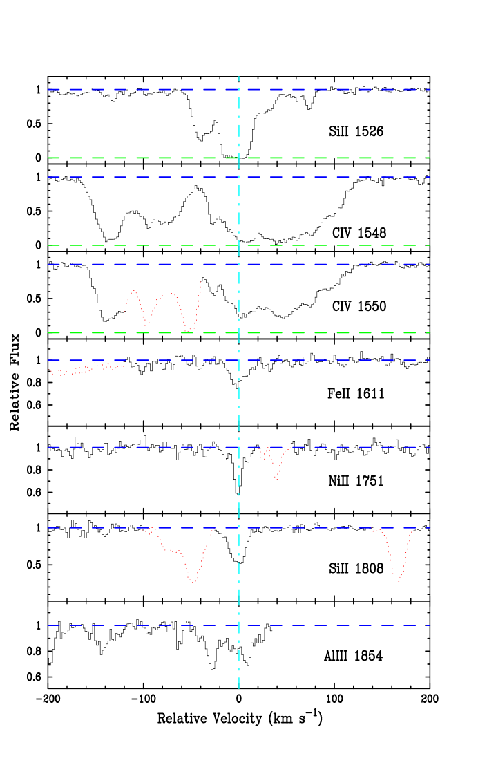
Figure 1.— Velocity plot of the metal-line transitions for the damped Ly$\alpha$ system at $z=3.390$ toward Q0000$-$26. The vertical line at $v=0$ corresponds to $z=3.3901$. Figures 2-21 are not included here but can be downloaded from: http://mamacass.ucsd.edu:8080/people/xavier/WWW/DLA/abundfig.ps.gz

3.2. Q0019$-$15, $z$ = 3.439

This damped Ly$\alpha$ system comes from the high redshift survey by Storrie-Lombardi et al. (1996) and the adopted $\log{N({\rm HI})}=20.9\pm 0.1$ was taken from recent Keck measurements of Storrie-Lombardi & Wolfe (1998). While our observations covered Ly$\alpha$ for this system, the profile extends over two echelle orders and an accurate measurement of ${N({\rm HI})}$ proved impossible. Figure 2 shows the metal-line transitions and Table 4 presents the measurements for this system. The Fe abundance is based on the marginally saturated FeII 1608 profile, yet should be reasonably accurate. The NiII lines are very weak and in poor SNR regions so these measurements are not reliable. The same is true for the Si measurements, although to a lesser extent. Note all of the high-ion profiles are blended with other metal-line transitions or Ly$\alpha$ forest clouds.

Table 4

Ionic Column Densities: Q0019$-$15, $z$ = 3.439 Ion $\lambda$ AODM $N_{adopt}$ [X/H] HI 1215 $20.900\pm 0.100$ SiII 1526 $>14.953$ $15.423\pm 0.053$ $-1.027\pm 0.113$ 1808 $15.423\pm 0.053$ SiIV 1402 $>14.495$ FeII 1608 $14.770\pm 0.064$ $14.770\pm 0.064$ $-1.640\pm 0.119$ NiII 1709 $13.300\pm 0.103$ $13.442\pm 0.043$ $-1.708\pm 0.109$ 1741 $13.442\pm 0.043$

3.3. Q0100$+$13, $z$ = 2.309

The majority of our results on PHL 957 (a.k.a. Q0100$+$13) were published by Wolfe et al. (1994). The major exception is we now present a measurement of the Fe abundance based on the previously unidentified FeII 1611 profile. Also, we measure column densities in light of new $f$ and $\lambda$ values, in particular those for the CrII and NiII transitions. Note the O abundance is based on the very weak OI 1355 profile and we report it as a $3\sigma$ upper limit. Figure 3 presents the velocity plots and Table 5 lists the measured ionic column densities for this system. This damped system is included in the statistical sample of the LBQS survey.

Table 5

Ionic Column Densities: Q0100$+$13, $z$ = 2.309 Ion $\lambda$ AODM $N_{adopt}$ [X/H] HI 1215 $21.400\pm 0.050$ CIV 1548 $13.241\pm 0.031$ 1550 $13.303\pm 0.056$ OI 1355 $<17.628$ $<17.628$ $<-0.702$ AlIII 1854 $12.635\pm 0.022$ 1862 $12.715\pm 0.033$ SiII 1526 $>14.722$ $>14.722$ $>-2.228$ SiIV 1393 $13.127\pm 0.017$ 1402 $13.146\pm 0.029$ CrII 2062 $13.389\pm 0.018$ $13.387\pm 0.015$ $-1.693\pm 0.052$ 2066 $13.383\pm 0.024$ FeII 1608 $>14.599$ $15.096\pm 0.041$ $-1.814\pm 0.065$ 1611 $15.096\pm 0.041$ NiII 1454 $13.621\pm 0.041$ $13.620\pm 0.014$ $-2.030\pm 0.052$ 1741 $13.620\pm 0.015$ ZnII 2026 $12.498\pm 0.028$ $12.494\pm 0.023$ $-1.556\pm 0.055$ 2062 $12.485\pm 0.039$

3.4. Q0149$+$33, $z$ = 2.140

This relatively metal-poor ([Fe/H] $\approx-1.8$ dex) damped system is a also member of the LBQS statistical sample. Table 6 gives the measured column densities and Figure 4 plots the metal-lines. In the following analysis, we assume $\log{N({\rm HI})}=20.5\pm 0.1$ (Wolfe et al. (1995)). As with PH957, the O abundance is based on the statistically insignificant OI 1355 profile and provides a very conservative upper limit. Finally the Al abundance is derived from the marginally saturated AlII 1670 profile but should be a reliable value. The system is notable for exhibiting an atypical Cr to Zn ratio; [Cr/Zn] $=+0.26\pm 0.1$ dex. The Cr measurement is reasonably accurate and the ZnII 2062 transition places a rather strict upper limit to the Zn abundance. Therefore, it is very likely [Cr/Zn] $>0$ which marks the first such occurrence in a damped system and indicates this system must be essentially undepleted.

Table 6

Ionic Column Densities: Q0149$+$33, $z$ = 2.140 Ion $\lambda$ AODM $N_{adopt}$ [X/H] HI 1215 $20.500\pm 0.100$ CI 1560 $<12.801$ CII 1334 $>14.623$ 1335 $<12.780$ CIV 1548 $13.880\pm 0.011$ 1550 $13.890\pm 0.017$ OI 1355 $<17.795$ $<17.795$ $<0.365$ AlII 1670 $12.936\pm 0.018$ $12.936\pm 0.018$ $-2.044\pm 0.102$ AlIII 1854 $12.518\pm 0.028$ 1862 $12.556\pm 0.043$ SiII 1304 $14.401\pm 0.042$ $14.367\pm 0.029$ $-1.683\pm 0.104$ 1526 $14.320\pm 0.034$ 1808 $14.572\pm 0.047$ SiIV 1393 $13.380\pm 0.017$ CrII 2056 $12.793\pm 0.044$ $12.811\pm 0.036$ $-1.369\pm 0.106$ 2062 $12.533\pm 0.087$ 2066 $12.853\pm 0.060$ FeII 1608 $14.202\pm 0.018$ $14.202\pm 0.018$ $-1.808\pm 0.102$ 1611 $<14.785$ NiII 1370 $12.920\pm 0.103$ $12.900\pm 0.042$ $-1.850\pm 0.108$ 1703 $<13.575$ 1709 $12.871\pm 0.088$ 1741 $12.990\pm 0.064$ 1751 $12.817\pm 0.090$ ZnII 2026 $11.496\pm 0.103$ $11.496\pm 0.103$ $-1.654\pm 0.144$ 2062 $<11.697$

3.5. Q0347$-$38, $z$ = 3.025

The damped Ly$\alpha$ system toward Q0347$-$38 is another member of the LBQS statistical sample, one of the four with $z_{abs}>3$. We adopt $\log{N({\rm HI})}=20.8\pm 0.1$ based on a measurement by Pettini et al. (1994). This is one of the few systems where we have an estimate of ${N({\rm S^{+}})}$, although we note SII 1259 is partially blended with the Ly$\alpha$ forest and should be considered an upper limit to the true S abundance, ${N({\rm S^{+}})}<10^{14.73}\,{\rm cm^{-2}}$. We discuss the S/Fe ratio in detail below, noting here that the value has particular impact on interpreting the abundances of the damped Ly$\alpha$ systems with respect to Type II SN enrichment and dust depletion. The system is also notable for the easily identifiable excited fine structure CII^∗ 1335 transition. Unfortunately, the CII 1334 profile is so heavily saturated that no meaningful comparison can be made with the fine structure transition. Finally, we observe a very low Ni abundance for this system, [Ni/H] $<-2.37$ dex, implying [Ni/Fe] $<-0.5$ dex which may be difficult to explain within the leading explanations for the damped Ly$\alpha$ abundance patterns.

Table 7

Ionic Column Densities: Q0347$-$38, $z$ = 3.025 Ion $\lambda$ AODM $N_{adopt}$ [X/H] HI 1215 $20.800\pm 0.100$ CII 1334 $>15.027$ $>15.027$ $>-2.333$ 1335 $13.477\pm 0.032$ CIV 1548 $13.846\pm 0.011$ 1550 $13.783\pm 0.020$ OI 1302 $>15.379$ $<17.740$ $<0.010$ 1355 $<17.740$ SiII 1260 $>14.268$ $14.820\pm 0.028$ $-1.530\pm 0.104$ 1304 $14.820\pm 0.028$ 1526 $>14.748$ SiIV 1393 $13.750\pm 0.017$ SII 1259 $14.731\pm 0.012$ $14.731\pm 0.012$ $-1.339\pm 0.101$ FeII 1608 $14.472\pm 0.007$ $14.472\pm 0.007$ $-1.838\pm 0.100$ 1611 $<14.476$ NiII 1370 $<12.677$ $<12.677$ $<-2.373$

3.6. Q0458$-$02, $z$ = 2.040

This damped Ly$\alpha$ system is ’famous’ for exhibiting HI 21cm absorption. In particular, Briggs et al. (1989) have used VLBI radio observations to place a lower limit on its size of 8 $h_{100}^{-1}$ kpc. In our analysis we adopt $\log{N({\rm HI})}=21.65\pm 0.09$ taken from Pettini et al. (1994). A plot of the metal-line profiles is given in Figure 6 and Table 8 lists the column densities. Note the CII^∗ 1335 profile is heavily saturated. Assuming the ${}^{2}P_{3/2}$ excited fine-structure state is populated by e^- collisions and ${N({\rm C^{+}})}<10^{17}\,{\rm cm^{-2}}$ (which follows by assuming [C/H] $<$ [Zn/H]), the limit on ${N({\rm CII^{*}})}$ indicates $n_{e}>0.1\,{\rm cm^{-3}}$. The system, with one of the highest measured ${N({\rm HI})}$ values, must have a high neutral fraction implying $n_{H}>0.1\,{\rm cm^{-3}}$. Because FeII 1608 is saturated, we base the Fe abundance on the FeII 1611 transition. Finally, we note the ZnII 2026 profile is blended with an unidentified line at $v>20{\rm\;km\;s^{-1}}$ and therefore the AODM was applied only to $v=+20{\rm\;km\;s^{-1}}$.

Table 8

Ionic Column Densities: Q0458$-$02, $z$ = 3.040 Ion $\lambda$ AODM $N_{adopt}$ [X/H] HI 1215 $21.650\pm 0.090$ CII 1334 $>15.010$ 1335 $>14.794$ CIV 1548 $>14.906$ 1550 $>15.111$ OI 1302 $>15.410$ 1355 $<18.560$ AlII 1670 $>13.720$ AlIII 1854 $13.334\pm 0.018$ 1862 $13.335\pm 0.022$ SiII 1304 $>15.095$ $>15.095$ $>-2.105$ 1526 $>14.981$ 1808 $>16.021$ SiIV 1393 $>14.262$ 1402 $>14.481$ CrII 2056 $13.756\pm 0.013$ $13.797\pm 0.008$ $-1.533\pm 0.090$ 2062 $13.763\pm 0.014$ 2066 $13.987\pm 0.015$ FeII 1608 $>15.136$ $15.508\pm 0.048$ $-1.652\pm 0.102$ 1611 $15.508\pm 0.048$ NiII 1317 $13.985\pm 0.024$ $13.853\pm 0.019$ $-2.047\pm 0.092$ 1709 $13.840\pm 0.035$ 1741 $13.936\pm 0.032$ 1751 $13.808\pm 0.033$ ZnII 2026 $13.141\pm 0.018$ $13.141\pm 0.018$ $-1.159\pm 0.092$

3.7. Q0841+12, $z$ = 2.375 & $z$ = 2.476

The damped Ly$\alpha$ systems toward this BL Lac object were first identified by C. Hazard and were subsequently analyzed by Pettini et al. (1997). We take ${N({\rm HI})}=20.95\pm 0.087$ for the system at $z=2.375$ and ${N({\rm HI})}=20.78\pm 0.097$ for the system at $z=2.476$ (Pettini et al. (1997)). Figures 7 and 8 plot the metal-line profiles for these systems and Tables 9 and 10 list the ionic column densities. The profiles for the lower redshift system have good SNR and the derived column densities are accurate. Unfortunately, its FeII 1608 and FeII 1611 transitions are blended with sky lines. In the abundance analysis, then, we will adopt an Fe abundance, [Fe/H] = [Cr/H], motivated by the fact that [Cr/Fe] $\approx$ 0 in the damped systems. For the system at $z=2.476$, SiII 1808 is blended with the AlIII 1862 transition from the $z=2.375$ system and also may be contaminated by a sky line. Therefore, we adopt a lower limit to ${N({\rm Si^{+}})}$ from the saturated SiII 1526 profile. Finally, we obtain an upper limit measurement for ${N({\rm Zn^{+}})}$ for this system which is a significant improvement over previous efforts (Pettini et al. (1997)).

Table 9

Ionic Column Densities: Q0841+12, $z$ = 2.375 Ion $\lambda$ AODM $N_{adopt}$ [X/H] HI 1215 $20.950\pm 0.087$ CIV 1548 $13.968\pm 0.011$ 1550 $13.973\pm 0.015$ AlII 1670 $>13.267$ $>13.267$ $>-2.163$ AlIII 1854 $12.504\pm 0.029$ 1862 $12.703\pm 0.035$ SiII 1526 $>14.566$ $15.239\pm 0.024$ $-1.261\pm 0.090$ 1808 $15.239\pm 0.024$ CrII 2056 $12.960\pm 0.061$ $13.079\pm 0.027$ $-1.551\pm 0.091$ 2062 $13.185\pm 0.034$ 2066 $13.035\pm 0.059$ NiII 1454 $13.211\pm 0.075$ $13.243\pm 0.030$ $-1.957\pm 0.092$ 1741 $13.297\pm 0.039$ 1751 $13.185\pm 0.055$ ZnII 2026 $12.114\pm 0.057$ $12.115\pm 0.049$ $-1.485\pm 0.100$ 2062 $12.115\pm 0.099$

Table 10

Ionic Column Densities: Q0841$+$12, $z$ = 2.476 Ion $\lambda$ AODM $N_{adopt}$ [X/H] HI 1215 $20.780\pm 0.097$ CIV 1548 $13.914\pm 0.009$ 1550 $13.986\pm 0.012$ AlII 1670 $13.186\pm 0.286$ $13.186\pm 0.286$ $-2.074\pm 0.302$ AlIII 1854 $12.683\pm 0.027$ 1862 $12.633\pm 0.038$ SiII 1526 $>14.461$ $>14.461$ $>-1.869$ 1808 $14.958\pm 0.022$ SiIV 1393 $13.646\pm 0.009$ 1402 $13.646\pm 0.011$ TiII 1910 $<12.434$ $<12.434$ $<-1.276$ CrII 2056 $12.907\pm 0.043$ $12.840\pm 0.036$ $-1.620\pm 0.103$ 2062 $12.759\pm 0.061$ 2066 $<12.802$ FeII 1608 $14.434\pm 0.027$ $14.434\pm 0.027$ $-1.856\pm 0.101$ 1611 $<14.668$ NiII 1741 $13.067\pm 0.052$ $13.048\pm 0.049$ $-1.982\pm 0.108$ 1751 $12.965\pm 0.129$ ZnII 2026 $<11.778$ $<11.778$ $<-1.652$ 2062 $<11.772$

3.8. Q0951$-$04, $z$ = 3.857 & $z$ = 4.203

The QSO Q0951$-$04 from the survey by Storrie-Lombardi et al. (1996) has two intervening damped Ly$\alpha$ systems, both at very high redshift. The velocity plots and measurements for the $z=3.857$ system are given in Figure 9 and Table 11, while those for the $z=4.203$ system are presented by Figure 10 and Table 12. We adopt $\log{N({\rm HI})}=20.6\pm 0.1$ for the system at $z=3.857$ and $\log{N({\rm HI})}=20.4\pm 0.1$ for the system at $z=4.203$, based on recent Keck measurements (Storrie-Lombardi and Wolfe (1998)). Because all of the column densities are based on either marginally saturated profiles or weaker, low SNR profiles all of these measurements are somewhat tentative. In fact, we consider the limits on ${N({\rm Fe^{+}})}$ for the system at $z=4.203$ to be too conservative to include this system in the abundance analysis. Finally, we note the feature at $v=180{\rm\;km\;s^{-1}}$ in the NiII 1370 profile for the $z=3.857$ system may be an unidentified blend, although it nearly coincides with a strong feature in the SiII 1526 profile.

Table 11

Ionic Column Densities: Q0951$-$04, $z$ = 3.857 Ion $\lambda$ AODM $N_{adopt}$ [X/H] HI 1215 $20.600\pm 0.100$ AlII 1670 $13.298\pm 0.022$ $13.298\pm 0.022$ $-1.782\pm 0.102$ SiII 1526 $14.645\pm 0.030$ $14.645\pm 0.030$ $-1.505\pm 0.104$ SiIV 1393 $13.900\pm 0.011$ FeII 1608 $14.062\pm 0.060$ $14.062\pm 0.060$ $-2.048\pm 0.117$ NiII 1370 $12.994\pm 0.099$ $12.994\pm 0.099$ $-1.856\pm 0.141$

Table 12

Ionic Column Densities: Q0951$-$04, $z$ = 4.203 Ion $\lambda$ AODM $N_{adopt}$ [X/H] HI 1215 $20.400\pm 0.100$ OI 1302 $14.607\pm 0.323$ $14.607\pm 0.323$ $-2.723\pm 0.339$ SiII 1190 $13.455\pm 0.050$ $13.392\pm 0.032$ $-2.558\pm 0.105$ 1304 $13.286\pm 0.060$ 1526 $13.483\pm 0.055$ FeII 1608 $<13.281$ $<13.281$ $<-2.629$ 1611 $<15.153$ NiII 1317 $<12.589$ $<12.589$ $<-2.061$ 1370 $<12.625$

3.9. Q1215$+$33, $z$ = 1.999

This radio-selected damped system (Wolfe et al. (1986)) was observed as part of the commissioning run for the HIRES instrument and is a member of the LBQS statistical sample. In the following analysis we assume $\log{N({\rm HI})}=20.95\pm 0.067$ based on observations by Pettini et al. (1994). Figure 11 presents a plot of the metal-line transitions and the ionic column densities are listed in Table 13. As the FeII 1608 profile is saturated and the FeII 1611 transition is marginally detected, we establish only a lower limit to ${N({\rm Fe^{+}})}$. We will include this system in the abundance analysis, however, by adopting $\log 10[{N({\rm Fe^{+}})}]=14.648\pm 0.033$ based solely on the FeII 1608 profile, noting this value may be an underestimate.

Table 13

Ionic Column Densities: Q1215$+$33, $z$ = 1.999 Ion $\lambda$ AODM $N_{adopt}$ [X/H] HI 1215 $20.950\pm 0.067$ CIV 1548 $13.605\pm 0.019$ 1550 $13.672\pm 0.030$ OI 1355 $<17.952$ $<17.952$ $<0.072$ AlII 1670 $>13.358$ AlIII 1854 $12.746\pm 0.017$ 1862 $12.783\pm 0.021$ SiII 1526 $>14.681$ $15.030\pm 0.025$ $-1.470\pm 0.072$ 1808 $15.030\pm 0.025$ SiIV 1393 $12.993\pm 0.039$ CrII 2056 $13.173\pm 0.034$ $13.130\pm 0.031$ $-1.500\pm 0.074$ 2062 $13.034\pm 0.066$ FeII 1608 $14.648\pm 0.039$ $14.648\pm 0.039$ $-1.812\pm 0.078$ 1611 $14.925\pm 0.100$ NiII 1741 $13.419\pm 0.040$ $13.344\pm 0.033$ $-1.856\pm 0.075$ 1751 $13.262\pm 0.056$ ZnII 2026 $12.291\pm 0.058$ $12.291\pm 0.058$ $-1.309\pm 0.089$

3.10. Q1331$+$17, $z$ = 1.776

This famous damped Ly$\alpha$ system which exhibits 21cm absorption (Wolfe & Davis (1979)) has been studied by a number of authors (over $100$ papers), yet never with the quality of data presented here (FWHM resolution $\approx 6{\rm\;km\;s^{-1}}$ and SNR $>$ 50). Table 14 lists the column densities for the metal-line transitions and Figure 12 plots their profiles. We assume $\log{N({\rm HI})}=21.176\pm 0.041$ (Pettini et al. (1994)). The SNR is excellent throughout the entire spectrum yielding very accurate column density measurements. This is one of the very few systems where CI absorption is detected and Songaila et al. (1994) have used measurements of the CI profile to estimate the cosmic background temperature at $z=1.776$. Consider the feature at $v=+20{\rm\;km\;s^{-1}}$ which is fully resolved in the CI profiles, barely resolved in the Zn⁺ profiles, and is unresolved in the stronger transitions even at 6 km s^-1 resolution. This suggest the gas in this component is at a temperature $T<6000$K. While this system may be atypical because it is one of the few damped systems to exhibit CI absorption, it is worth noting a majority of observed damped Ly$\alpha$ profiles may be the result of the superposition of many narrow components.

Table 14

Ionic Column Densities: Q1331$+$17, $z$ = 1.776 Ion $\lambda$ AODM $N_{adopt}$ [X/H] HI 1215 $21.176\pm 0.041$ CI 1560 $13.573\pm 0.013$ 1656 $13.312\pm 0.012$ CIV 1548 $>15.073$ 1550 $>15.172$ AlII 1670 $>13.573$ AlIII 1854 $13.004\pm 0.004$ 1862 $12.968\pm 0.007$ SiII 1526 $>14.951$ $15.285\pm 0.004$ $-1.441\pm 0.041$ 1808 $15.285\pm 0.004$ CrII 2056 $12.950\pm 0.017$ $12.919\pm 0.015$ $-1.937\pm 0.044$ 2066 $12.834\pm 0.034$ FeII 1608 $14.601\pm 0.003$ $14.598\pm 0.001$ $-2.088\pm 0.041$ 2344 $14.597\pm 0.022$ 2374 $14.598\pm 0.002$ 2382 $>14.433$ NiII 1709 $13.166\pm 0.017$ $13.235\pm 0.009$ $-2.191\pm 0.042$ 1741 $13.313\pm 0.011$ 1751 $13.165\pm 0.022$ ZnII 2026 $12.605\pm 0.009$ $12.605\pm 0.008$ $-1.221\pm 0.042$ 2062 $12.605\pm 0.013$

3.11. Q1346$-$03, $z$ = 3.736

This very high $z$ damped Ly$\alpha$ system was taken from the survey of Storrie-Lombardi et al. (1996). We present the velocity plots and column densities in Figure 13 and Table 15. We adopt $\log{N({\rm HI})}=20.7\pm 0.1$ (Storrie-Lombardi and Wolfe (1998)) throughout the analysis. Unfortunately both FeII 1608 and FeII 1611 are blended with B-band sky lines. Therefore, we have no metallicity indicator for this system and it is not included in the subsequent analysis. Measuring [Si/H] = $-2.3$ dex, we expect this is a very metal-poor system.

Table 15

Ionic Column Densities: Q1346$-$03, $z$ = 3.736 Ion $\lambda$ AODM $N_{adopt}$ [X/H] HI 1215 $20.700\pm 0.100$ CII 1334 $14.422\pm 0.095$ $14.422\pm 0.095$ $-2.838\pm 0.138$ AlII 1670 $12.546\pm 0.025$ $12.546\pm 0.025$ $-2.634\pm 0.103$ SiII 1304 $13.961\pm 0.012$ $13.954\pm 0.011$ $-2.296\pm 0.101$ 1526 $13.923\pm 0.026$ SiIV 1393 $12.344\pm 0.096$ 1402 $<12.598$ NiII 1370 $<12.694$ 1741 $<13.024$

3.12. Q1759$+$75, $z$ = 2.625

This system and the adopted ${N({\rm HI})}=20.8\pm 0.1$ are taken from an ongoing survey by I. Hook. Figure 14 presents the velocity plots and Table 16 gives the measurements. The QSO is very bright and was observed at FWHM $\approx 6{\rm\;km\;s^{-1}}$ resolution. We expect all of the measured abundances are very accurate with the exception of ${N({\rm Zn^{+}})}$ where the ZnII 2026 profile is blended with sky lines. Although the strongest feature appears unblended, we have chosen not to include Zn in the abundance analysis.

Table 16

Ionic Column Densities: Q1759$+$75, $z$ = 2.625 Ion $\lambda$ AODM $N_{adopt}$ [X/H] HI 1215 $20.800\pm 0.100$ CIV 1548 $14.636\pm 0.019$ 1550 $14.647\pm 0.005$ AlIII 1854 $13.623\pm 0.004$ SiII 1526 $>15.014$ $15.532\pm 0.008$ $-0.818\pm 0.100$ 1808 $15.532\pm 0.008$ CrII 2066 $13.211\pm 0.062$ $13.211\pm 0.062$ $-1.269\pm 0.117$ FeII 1608 $>14.980$ $15.076\pm 0.042$ $-1.234\pm 0.108$ 1611 $15.076\pm 0.042$ NiII 1454 $13.589\pm 0.039$ $13.565\pm 0.011$ $-1.485\pm 0.101$ 1709 $13.615\pm 0.020$ 1741 $13.582\pm 0.017$ 1751 $13.506\pm 0.021$ ZnII 2026 $>11.650$ $>11.650$ $>-1.800$

3.13. Q2230$+$02, $z$ = 1.864

Figure 15 presents the velocity plots for the damped Ly$\alpha$ system toward Q2230$+$02 and Table 17 lists the measured ionic column densities. We adopt $\log{N({\rm HI})}=20.85\pm 0.084$ (Pettini et al. (1994)) for this LBQS damped system. We have wavelength coverage of 28 metal-line transitions and have determined accurate column densities for the majority of them. This system is notable for a $4\sigma$ detection of ${N({\rm Ti^{+}})}$. There are two TiII transitions at 1910   Åwith similar oscillator strengths and the profiles cannot be disentangled. Following the analysis presented in Prochaska & Wolfe (1997a), we integrate $N_{a}$ over the entire velocity region associated with the TiII transitions and use a reduced oscillator strength, $f^{*}\equiv(f_{1}^{2}+f_{2}^{2})/(f_{1}+f_{2})=0.0862$, to calculate ${N({\rm Ti^{+}})}$. There is another difficulty in determining the Ti⁺ column density for this system. An emission line feature lies just blueward of the TiII profiles and causes problems in determining the continuum level. This leads to a systematic error estimated at 0.1 dex.

The profile for the low-ion transitions is comprised of three primary features whose relative optical depth apparently varies from transition to transition. For instance, the central feature is the strongest in the SiII 1808, CrII 2062, CrII 2066, and ZnII 2026 profiles and the weakest in the FeII 2260 and CrII 2056 transitions. While differences in the level of dust depletion could account for some of the variations, it would be impossible to explain the differences for a single ion (e.g. the CrII transitions). The most likely explanation is that this central feature is a very narrow component – not fully resolved at our resolution – whose relative optical depth varies significantly with the strength of the transition. Finally, this system is notable for the presence of a nearby metal-line system at $\approx-550{\rm\;km\;s^{-1}}$ which shows multiple metal transitions (Figure 16). The subsystem exhibits ionic column densities typical of a damped Ly$\alpha$ system and its Al⁺/Al${}^{++}=2.6$ ratio indicates the system is nearly neutral. Therefore, it is almost certainly contributing to the measured ${N({\rm HI})}$ for this system which would mean we are underestimating the metallicity of the system at $z=1.864$. Because the nearby system exhibits ionic column densities at $<10\%$ of the damped system, we have chosen to ignore its effects in our abundance analysis.

Table 17

Ionic Column Densities: Q2230$+$02, $z$ = 1.864 Ion $\lambda$ AODM $N_{adopt}$ [X/H] HI 1215 $20.850\pm 0.084$ CIV 1548 $>14.848$ 1550 $14.808\pm 0.007$ AlII 1670 $>14.020$ AlIII 1854 $13.590\pm 0.006$ 1862 $13.596\pm 0.009$ SiII 1526 $>15.233$ $15.656\pm 0.010$ $-0.744\pm 0.085$ 1808 $15.656\pm 0.010$ SiIV 1393 $>14.267$ 1402 $>14.354$ TiII 1910 $12.985\pm 0.099$ $12.985\pm 0.099$ $-0.795\pm 0.130$ CrII 2056 $13.361\pm 0.036$ $13.403\pm 0.027$ $-1.127\pm 0.088$ 2066 $13.483\pm 0.041$ FeII 1608 $>15.115$ $15.188\pm 0.016$ $-1.172\pm 0.086$ 1611 $15.273\pm 0.084$ 2249 $15.120\pm 0.036$ 2260 $15.210\pm 0.019$ 2344 $>14.988$ 2374 $>15.183$ 2382 $>14.723$ NiII 1370 $13.883\pm 0.052$ $13.812\pm 0.011$ $-1.288\pm 0.085$ 1709 $13.860\pm 0.014$ 1741 $13.838\pm 0.023$ 1751 $13.687\pm 0.028$ ZnII 2026 $12.800\pm 0.028$ $12.800\pm 0.028$ $-0.700\pm 0.088$

3.14. Q2231$-$00, $z$ = 2.066

This LBQS system is another damped Ly$\alpha$ system exhibiting significant $(5\sigma)$ TiII 1910 absorption. As in the damped Ly$\alpha$ system toward Q2230$+$02, the TiII profiles overlap, hence we use the technique outlined above to determine ${N({\rm Ti^{+}})}$. Throughout the analysis we adopt $\log{N({\rm HI})}=20.56\pm 0.1$ (Pettini et al. (1994)). The velocity plots are given in Figure 17 and the column densities are presented in Table 18. This is the other system in our data sample which was previously observed by Lu et al. (1996). We find our measurements match theirs in nearly every case, although their analysis did not include Ti⁺.

Table 18

Ionic Column Densities: Q2231$-$00, $z$ = 2.066 Ion $\lambda$ AODM $N_{adopt}$ [X/H] HI 1215 $20.560\pm 0.100$ CII 1335 $13.580\pm 0.040$ CIV 1548 $14.195\pm 0.005$ OI 1302 $>15.543$ $<17.748$ $<0.258$ 1355 $<17.748$ AlIII 1854 $13.172\pm 0.010$ 1862 $13.110\pm 0.023$ SiII 1304 $>15.030$ $15.247\pm 0.019$ $-0.863\pm 0.102$ 1526 $>15.014$ 1808 $15.247\pm 0.019$ SiIV 1393 $13.704\pm 0.010$ 1402 $13.698\pm 0.012$ TiII 1910 $12.848\pm 0.071$ $12.848\pm 0.071$ $-0.642\pm 0.123$ CrII 2062 $13.182\pm 0.040$ $13.165\pm 0.034$ $-1.075\pm 0.106$ 2066 $13.130\pm 0.063$ FeII 1608 $14.750\pm 0.009$ $14.750\pm 0.009$ $-1.320\pm 0.100$ 1611 $14.783\pm 0.065$ NiII 1370 $12.880\pm 0.091$ $13.306\pm 0.032$ $-1.504\pm 0.105$ 1741 $13.381\pm 0.033$ 1751 $13.100\pm 0.091$ ZnII 2026 $12.463\pm 0.023$ $12.463\pm 0.023$ $-0.747\pm 0.103$

3.15. Q2348$-$14, $z$ = 2.279

This very metal-poor system was first discussed by Pettini et al. (1994) and has been previously observed at high resolution by Pettini et al. (1995). In Figure 19 we plot the Ly$\alpha$ transition for this system. Overplotted are Voigt profiles centered at $z=2.2794$ with $\log{N({\rm HI})}=20.56\pm 0.075$ corresponding to the measurements made by Pettini et al. (1994). While the profiles provide a reasonable fit to the left wing of the damped profile, the fit for $v>750{\rm\;km\;s^{-1}}$ is clearly inconsistent for all of the assumed ${N({\rm HI})}$ values. It is very difficult, however, to continuum fit an order of HIRES data which includes a damped Ly$\alpha$ profile; it is easier to fit intermediate resolution data. Therefore, we adopt $\log{N({\rm HI})}=20.56\pm 0.075$ from the Pettini et al. analysis, but note in passing that this may be an overestimate of the true ${N({\rm HI})}$ value. Comparing our derived chemical abundances with the work of Pettini et al. (1995) we find reasonable agreement and note we have improved on their limits in a few cases (e.g. N and S).

The system is exceptional for a number of reasons. First, it is one of the few systems where we have a measurement of ${N({\rm S^{+}})}$ based on the SII 1259 transition. As discussed for the damped system toward Q0347$-$38, S/Fe is an excellent diagnostic of dust depletion. Here we find [S/Fe] = 0.17 dex which argues strongly against dust depletion if the system has an underlying Type II SN pattern. Second, the system exhibits two distinct low-ion features, one at $v\approx-100{\rm\;km\;s^{-1}}$ (feature 1; this feature was not resolved in previous observations) and the more dominant at $v\approx 0{\rm\;km\;s^{-1}}$ (feature 2). Feature 1 is present in all of the SiII transitions and is the strongest feature in the AlIII, CIV and SiIV profiles. Comparing ${N({\rm Si^{+}})}$ for the two features in the SiII 1526 profile, we find ${N({\rm Si^{+}})}_{1}/{N({\rm Si^{+}})}_{2}=0.18$. At the same time, however, the feature is entirely absent in the OI 1302 and FeII 1608 profiles: ${N({\rm O^{0}})}_{1}/{N({\rm O^{0}})}_{2}<0.027$ and ${N({\rm Fe^{+}})}_{1}/{N({\rm Fe^{+}})}_{2}<0.07$. While dust could possibly explain the absence of Fe where Si is present because Si is only lightly depleted in the ISM, it cannot account for the lack of OI absorption. The system corresponding to feature 1 must be significantly ionized such that the dominant states of O, Fe, and Si are higher ions. We have performed CLOUDY (Ferland (1991)) calculations which demonstrate values of [Si⁺/O⁰] $\approx 1.2$ dex and [Si⁺/Fe⁺] $\approx 0.7$ dex are possible in a Lyman limit system provided the ionization parameter is significantly high. Therefore, we argue feature 2 marks the damped Ly$\alpha$ system while feature 1 may be a significantly ionized satellite or halo cloud. The system is also notable for providing a meaningful estimate of N/O. Finally, perhaps the most remarkable characteristic of this damped system is the velocity width of the CIV profiles, $\Delta v>600{\rm\;km\;s^{-1}}$, particularly in light of the very narrow $\Delta v$ exhibited by the low-ion profiles. This kinematic observation poses a difficult challenge to any physical model introduced to explain the damped Ly$\alpha$ systems.

Table 19

Ionic Column Densities: Q2348$-$14, $z$ = 2.279 Ion $\lambda$ AODM $N_{adopt}$ [X/H] HI 1215 $20.560\pm 0.075$ CII 1334 $>14.610$ 1335 $13.207\pm 0.070$ NI 1200 $<13.223$ $<13.223$ $<-3.387$ OI 1302 $>14.798$ $>14.798$ $>-2.692$ AlII 1670 $12.654\pm 0.006$ $12.654\pm 0.006$ $-2.386\pm 0.075$ AlIII 1854 $12.726\pm 0.012$ 1862 $12.613\pm 0.027$ SiII 1190 $>14.207$ $14.201\pm 0.010$ $-1.909\pm 0.076$ 1193 $>13.924$ 1260 $>13.744$ 1304 $14.227\pm 0.021$ 1526 $14.201\pm 0.011$ 1808 $14.089\pm 0.059$ SiIV 1393 $>14.063$ SII 1259 $13.725\pm 0.119$ $13.725\pm 0.119$ $-2.105\pm 0.140$ FeII 1608 $13.792\pm 0.016$ $13.792\pm 0.016$ $-2.278\pm 0.077$

3.16. Q2359$-$02, $z$=2.095 & $z$=2.154

This faint QSO exhibits two intervening damped Ly$\alpha$ systems. Both are members of the LBQS statistical survey. The velocity plots and column densities for the $z=2.095$ system are presented in Figure 20 and Table 20 and those for the $z=2.154$ are given by Figure 21 and Table 21. Both are part of the LBQS statistical sample and we have taken the HI column densities from Wolfe et al. (1995): $\log{N({\rm HI})}=20.7\pm 0.1$ for the $z=2.095$ system and $\log{N({\rm HI})}=20.3\pm 0.1$ for the $z=2.154$ system. The SNR is relatively low for most of the spectrum and therefore abundances established on the weakest transitions are suspect, particularly those for Zn. We intend to make further observations of these two systems to improve the accuracy of our abundance measurements.

Table 20

Ionic Column Densities: Q2359$-$02, $z$ = 2.095 Ion $\lambda$ AODM $N_{adopt}$ [X/H] HI 1215 $20.700\pm 0.100$ CII 1334 $>15.146$ CIV 1548 $>14.639$ 1550 $>14.800$ AlII 1670 $13.662\pm 0.034$ $13.662\pm 0.034$ $-1.518\pm 0.106$ AlIII 1854 $13.383\pm 0.010$ 1862 $13.396\pm 0.016$ SiII 1526 $>15.045$ $15.408\pm 0.021$ $-0.842\pm 0.102$ 1808 $15.408\pm 0.021$ SiIV 1393 $>14.072$ 1402 $>14.517$ CrII 2056 $12.748\pm 0.091$ $12.748\pm 0.091$ $-1.632\pm 0.135$ 2062 $13.131\pm 0.057$ 2066 $<12.897$ FeII 1608 $14.507\pm 0.025$ $14.507\pm 0.025$ $-1.703\pm 0.103$ 1611 $<15.077$ NiII 1703 $<13.693$ $13.142\pm 0.054$ $-1.808\pm 0.114$ 1709 $13.152\pm 0.127$ 1741 $13.185\pm 0.072$ 1751 $13.071\pm 0.107$ ZnII 2026 $12.595\pm 0.029$ $12.595\pm 0.029$ $-0.755\pm 0.104$ 2062 $12.486\pm 0.075$

Table 21

Ionic Column Densities: Q2359$-$02, $z$ = 2.154 Ion $\lambda$ AODM $N_{adopt}$ [X/H] HI 1215 $20.300\pm 0.100$ CII 1334 $>14.987$ CIV 1548 $>14.880$ 1550 $>14.966$ AlII 1670 $13.165\pm 0.016$ $13.165\pm 0.016$ $-1.615\pm 0.101$ AlIII 1862 $12.960\pm 0.021$ SiII 1526 $14.316\pm 0.015$ $14.316\pm 0.015$ $-1.534\pm 0.101$ SiIV 1393 $>14.568$ 1402 $>14.528$ CrII 2056 $<12.549$ $<12.946$ $<-1.034$ 2066 $<12.946$ FeII 1608 $13.895\pm 0.032$ $13.895\pm 0.032$ $-1.915\pm 0.105$ 1611 $<14.917$ NiII 1317 $<13.152$ $<12.949$ $<-1.601$ 1370 $<13.248$ 1454 $<13.063$ 1741 $<12.949$ 1751 $<13.200$ ZnII 2026 $<11.901$ $<11.901$ $<-1.049$

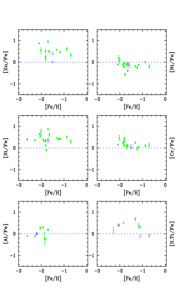
Figure 22.— Abundance patterns of the most common elements from our full damped Ly$\alpha$ sample. Following standard practice in stellar abundance analysis we plot [X/Fe], the logarithmic abundance of element X to Fe relative to solar. We plot this quantity vs. [Fe/H], an indicator of the metallicity of the system. The triangles printed in each panel represent the typical metal-poor halo value (McWilliam (1997)). The circles indicate the observed pattern for lightly depleted ISM gas (Savage and Sembach (1996)). In the lower right panel, the $x$’s identify [S/Fe] values and the squares mark [Ti/Fe].

Table 22

DLA	$z_{abs}$	log[N(HI)]	[Si/H]	[Al/H]	[S/H]	[Fe/H]	[Ni/H]	[Cr/H]	[Zn/H]
Q0000$-$26	3.390	21.410	$-1.874$			$-1.774$	$-2.335$
Q0019$-$01	3.439	20.900	$-1.027$			$-1.640$	$-1.708$
Q0100+13	2.309	21.400	$>-2.228$			$-1.814$	$-2.030$	$-1.693$	$-1.556$
Q0149+33	2.141	20.500	$-1.683$	$-2.044$		$-1.808$	$-1.850$	$-1.369$	$-1.654$
Q0201+36	2.463	20.380	$-0.376$			$-0.878$	$-0.877$	$-0.776$	$-0.266$
Q0347$-$38	3.025	20.800	$-1.530$		$-1.339$	$-1.838$	$<-2.373$
Q0458$-$02	2.040	21.650	$>-2.105$			$-1.652$	$-2.047$	$-1.533$	$-1.159$
Q0841+12A	2.375	20.950	$-1.261$	$>-2.163$		$-2.015$	$-1.957$	$-1.551$	$-1.485$
Q0841+12B	2.476	20.780	$>-1.869$	$-2.074$		$-1.856$	$-1.982$	$-1.620$	$<-1.652$
Q0951$-$04A	3.857	20.600	$-1.505$	$-1.782$		$-2.048$	$-1.856$
Q0951$-$04B	4.203	20.400	$-2.558$			$<-2.629$	$<-2.061$
Q1215+33	1.999	20.950	$-1.470$			$-1.812$	$-1.856$	$-1.500$	$-1.309$
Q1331+17	1.776	21.176	$-1.441$			$-2.088$	$-2.191$	$-1.937$	$-1.221$
Q1346$-$03	3.736	20.700	$-2.296$	$-2.634$
Q1759+75	2.625	20.800	$-0.818$			$-1.234$	$-1.485$	$-1.269$	$>-1.800$
Q2206$-$19A	1.920	20.653	$-0.402$			$-0.705$	$-0.903$	$-0.580$	$-0.379$
Q2206$-$19B	2.076	20.431	$-2.225$	$-2.727$		$-2.621$
Q2230+02	1.864	20.850	$-0.744$			$-1.172$	$-1.288$	$-1.127$	$-0.700$
Q2231$-$00	2.066	20.560	$-0.863$			$-1.320$	$-1.504$	$-1.075$	$-0.747$
Q2348$-$14	2.279	20.560	$-1.909$	$-2.386$	$-2.105$	$-2.278$
Q2359$-$02A	2.095	20.700	$-0.842$	$-1.518$		$-1.703$	$-1.808$	$-1.632$	$-0.755$
Q2359$-$02B	2.154	20.300	$-1.534$	$-1.615$		$-1.915$	$<-1.601$	$<-1.034$	$<-1.049$

4. ABUNDANCE PATTERNS

Table 22 lists the relative logarithmic abundances for the damped Ly$\alpha$ systems, [X/H] $\equiv\log[{N({\rm X})}/{N({\rm H})}]-\log[{N({\rm X})}/{N({\rm H})}]_{\odot}$. For each system we adopt the value for ${N({\rm HI})}$ indicated in the previous section, and calculate ${N({\rm X})}$ by performing a weighted mean of all direct measurements, i.e. no limits or blends. Included in Table 22 are the abundance measurements for the damped Ly$\alpha$ systems toward Q0201$+$36 and Q2206$-$19. In a few cases the values differ from the published values in light of new oscillator strengths. It is well-established both observationally and theoretically that the damped Ly$\alpha$ systems are primarily neutral (Viegas (1994); Prochaska & Wolfe (1996)). Therefore we perform no ionization corrections in determining the abundances from the ionic column densities of the low-ions.

Figure 22 presents the abundance patterns for the most common elements in our full sample. We have chosen not to include error bars for presentation purposes; the derived errors are $<0.1$ dex with only a few exceptions. Following Lu et al. (1996), along the x-axis of each panel we plot metallicity – here expressed with [Fe/H] – in part because this is the primary metallicity indicator in local stellar populations and in part because we have Fe abundance measurements for a greater number of systems. Examining the upper-left panel of Figure 22, we note a systematic overabundance of Zn/Fe which suggests Fe may be depleted onto dust grains. Therefore consider the [Fe/H] values to be lower limits to the true metallicity. In one case where (Q0841+12A) we have no reliable Fe abundance measurement and have taken [Fe/H] = [Cr/H] on the grounds that [Cr/H] $\approx$ [Fe/H] in the majority of damped Ly$\alpha$ systems.

In the following, we discuss the evidence for dust depletion and Type II supernovae enrichment in light of the observed damped Ly$\alpha$ abundance patterns. The former is determined by comparing against abundance patterns in depleted ISM clouds (Savage and Sembach (1996)) while the latter is assessed by comparing against the abundance patterns of metal-poor halo stars presumed to exhibit nucleosynthetic patterns typical of Type II supernovae (McWilliam (1997)). First, consider the top two panels of Figure 22 which lend support to the presence of significant dust depletion in the damped Ly$\alpha$ systems. As described throughout the paper, the overabundance of Zn to Fe relative to solar abundances is suggestive of dust depletion both because (i) Zn is largely undepleted in dusty regions within the ISM whereas Fe is heavily depleted and (ii) [Zn/Fe] $\approx 0$ dex for stars of all metallicity observed within the Galaxy (Sneden et al. (1991)). Similarly, the Ni/Fe ratio is significantly lower than metal-poor halo stars, which is consistent with Ni being more heavily depleted than Fe in depleted regions of the ISM. Lu et al. (1996) have argued the underabundance is primarily due to an error in the oscillator strengths for the NiII transitions. While a recent analysis by Zsarg$\rm\acute{o}$ & Federman (1998) indicates the NiII $f$-values are poorly determined, it is not clear if this can entirely account for the discrepancy between the damped Ly$\alpha$ observations and the metal-poor halo star abundances. For our analysis, we have adopted the updated $f$-values from Zsarg$\rm\acute{o}$ & Federman (1998) – which does include a decrease in $f_{1714}$ by a factor of 1.34 – yet a significant underabundance of [Ni/Fe] is still apparent. Therefore it is unclear if errors in the oscillator strengths can fully resolve the discrepancy between the observed Ni/Fe pattern and that predicted for Type II SN yields.

In contrast to the top two panels, the middle panels and the Al/Fe abundance pattern are generally consistent with both dust depletion and Type II SN enrichment. As emphasized by Lu et al. (1996), the overabundance of Si/Fe relative to solar is very suggestive of Type II supernovae enrichment (McWilliam (1997)). In the case of Si/Fe, the Si overabundance is explained as the result of the overproduction of Si – an $\alpha$-element relative to Fe in Type II supernovae. Similarly, the Cr/Fe and Al/Fe patterns are consistent with those observed for the metal-poor halo stars. Contrary to the Lu et al. observations, however, we observe an overabundance of Cr/Fe at very low metallicity (for [Fe/H] $<-1.5$, $<$[Cr/Fe]$>=+0.21$). This result is most likely due to the fact that we are biased to high [Cr/Fe] values at low [Fe/H] because low [Cr/Fe] values would imply Cr⁺ column densities below our detection limit. In one system (Q0149+33) we observe [Cr/Zn] $>0$ dex indicating it is essentially undepleted by dust grains. Furthermore, we measure an overabundance of Si relative to Fe in this system ([Si/Fe] = $+0.12$ dex) which is an indication of a Type II $\alpha$-enhancement although at a somewhat smaller level than most metal-poor halo stars. Lastly, while the [Al/Fe] measurements are broadly consistent with the abundances observed in metal-poor halo stars, there may be a contradiction at very low [Fe/H]. For halo stars with [Fe/H] $<-2$ dex, [Al/Fe] $<-0.4$ dex; McWilliam (1997)) yet if anything the damped Ly$\alpha$ systems exhibit [Al/Fe] $>0$ dex at this metallicity. This result may ultimately pose a serious challenge to the interpretation of Type II SN nucleosynthetic patterns.

Figure 23.— [Si/Fe], [Zn/Fe] pairs for the 9 damped Ly$\alpha$ systems from the full sample exhibiting Si, Zn, and Fe. The positive correlation (Pearson’s correlation coeffecient $r=0.86$ with the null hypothesis a 0.003 probability) is suggestie of dust depletion, but could possibly have a nucleosynthetic origin (see text).

While the abundances for Cr, Al and Si vs. Fe resemble those for the metal-poor halo stars, the patterns also tend to match the dust depletion patterns of lightly depleted regions within the ISM (Savage and Sembach (1996)). In these regions, Si is overabundant relative to Fe, [Cr/Fe] $\approx 0.1$ dex, and recent measurements of the Al to Fe ratio towards three OB stars (Howk & Savage (1998)) suggest [Al/Fe] $\gtrsim 0$ dex. If the overabundance of Si/Fe relative to solar is indicative of dust depletion, then one might expect a correlation between [Si/Fe] and [Zn/Fe] with the most heavily depleted regions showing the largest Si/Fe and Zn/Fe ratios. A plot of [Si/Fe] vs. [Zn/Fe] for all the systems with accurate abundances for the three elements (Figure 23) reveals a positive correlation (the Pearson coeffecient is 0.86 in log-space with a null hypothesis probability of 0.003), consistent with that expected for dust depletion. However, if Zn is produced in the neutrino-driven winds of Type II SN (Hoffman et al. (1996)), one may also expect a correlation between the abundance of Si and Zn relative to Fe.

Now consider the observations of Ti/Fe (solid squares in the lower right hand panel) which pose a strong argument for Type II SN enrichment. As emphasized in Prochaska & Wolfe (1997a), Ti is more heavily depleted than Fe in dusty regions within the ISM (Lipman & Pettini (1995)), yet we find [Ti/Fe] $\geq 0$ in every damped Ly$\alpha$ systems where Ti is observed. As Ti is an $\alpha$-element, this argues strongly for the Type II SN interpretation. Lu et al. (1996) have made similar arguments for the observed underabundance of Mn/Fe in the damped systems. Because Mn is less depleted than Fe in dusty regions of the ISM, the Mn/Fe underabundance cannot be explained by dust depletion. On the other hand one observes [Mn/Fe]$<0$ dex for the metal-poor halo stars (McWilliam (1997)). Furthermore, the [Mn/Fe] values show a similar trend with [Fe/H] (albeit in terms of an underabundance) to that of the $\alpha$-elements. It is possible this trend indicates a metallicity dependent yield for Mn, but the plateau in [Mn/Fe] values at [Fe/H] $\approx-1$ to $-2.5$ is better understood if Mn is overproduced relative to Fe by Type Ia supernovae (Nakamura et al. (1998)). If the latter explanation is correct, then the low [Mn/Fe] values are significant evidence for Type II SN enrichment within the damped Ly$\alpha$ systems. At the very least, we wish to stress the damped [Mn/Fe] observations require that the underlying nucleosynthetic pattern does not simply match solar abundances.

For the elements considered thus far, the abundance patterns are broadly consistent with a combination of Type II SN enrichment and an ’ISM-like’ dust depletion pattern. This is not the case for Sulphur. In the two cases from our full sample where we have accurate measurements for S/Fe we find: (i) [S/Fe] = $0.50\pm 0.02$ for the damped system at $z=3.025$ toward Q0347$-$38 and (ii) [S/Fe] = $0.17\pm 0.1$ for the damped system toward Q2348$-$14. Similar to Silicon, Sulfur is an $\alpha$-element and is observed to be overabundant relative to Fe in metal-poor halo stars by [Si/Fe]${}_{II}\approx 0.3-0.5$ dex. Like Zinc, Sulfur is undepleted in the ISM. Therefore, interpreting the positive [Zn/Fe] values as the result of dust depletion, one would expect typical values for [S/Fe]_dust $>0.3$ dex on the basis of depletion alone. Given all of the damped systems – including those from Lu et al. (1996) – exhibit [S/Fe] $\leq 0.5$ dex, the S abundance pattern is inconsistent with a combination of Type II SN enrichment and dust depletion because this would require [S/Fe]_obs = [S/Fe]_II + [S/Fe]${}_{dust}>0.6$ dex in every case. While this point has been discussed previously, it needs to be emphasized. If dust is playing the primary role in the observed abundance patterns of the damped Ly$\alpha$ systems, then the [S/Fe] measurements require one of two conclusions: (1) the damped Ly$\alpha$ systems were not primarily enriched by Type II SN or (2) all of the systems where S has been measured are atypical in that they are the few which are undepleted. The first conclusion is at odds with most theories of galactic chemical evolution and is inconsistent with the observations of the Milky Way. To adopt point (1), one would have to argue the chemical history of the damped systems is very different from that of the Milky Way. Point (2) is a possibility for Q2348$-$14, but the Ni/Fe ratio observed for Q0347$-$38 ([Ni/Fe] $<-0.5$) would indicate this system is significantly depleted. At present, then, any attempt to match the abundance patterns of the damped Ly$\alpha$ systems with a combination of Type II SN enrichment and ISM-like dust depletion must fail the S observations.

Synthesizing our results with those from previous studies, we contend the abundance patterns of the damped Ly$\alpha$ systems lack any convincing single interpretation. On the face of it this may not be surprising, as one would expect some differences in their chemical evolution. While this would explain variations of a particular X/Fe ratio, this is unlikely to account for any of the inconsistencies discussed thus far. While the majority of the patterns are in excellent agreement with the Type II SN enriched halo star abundance patterns, Zn/Fe and Ni/Fe are clearly inconsistent and are very suggestive of dust depletion, albeit at considerably lower levels than that observed in dusty ISM clouds. An ’ISM-like’ dust depletion pattern on top of solar abundances accounts for a majority of the observations but fails for Mn/Fe and Ti/Fe. Attempts to match the observed abundance patterns with a combination of dust depletion and Type II supernovae enrichment have been largely unsuccessful (Lu et al. (1996); Kulkarni et al. (1997); Vladilo (1998)). This failure is accentuated by our measurements of [S/Fe] which are inconsistent with a synthesis of dust depletion and Type II SN abundance patterns. Of course to eliminate either effect would have profound consequences. If the damped Ly$\alpha$ systems do not exhibit Type II SN abundances they have a very different chemical evolution history than the Milky Way, in that they do not match the stellar abundance patterns for [Fe/H] $<-1$ dex. This would beg the questions: Is the Milky Way unique? Or do the damped Ly$\alpha$ systems somehow not include the progenitors of present-day spiral galaxies? Also, why would the damped systems exhibit relative solar abundances for all elements except Mn and Ti? On the other hand, if there is no dust depletion at play, then is the Zn/Fe ratio observed in the Milky Way a special case? Also, are the [Al/Fe] observation at low metallicity consistent with the Type II SN interpretation?

At the heart of these questions lies the physical nature of the damped Ly$\alpha$ systems. If dust depletion is playing a principal role, then perhaps the damped systems are tracing gas-rich galaxies not unlike the Magellanic Clouds (Welty et al. (1997)), whereas an underlying Type II SN pattern is more suggestive of the progenitors of massive spiral galaxies. What steps can be taken to resolve these issues? First, the overabudance of Ti/Fe must be confirmed. A more accurate measurement of the TiII 1910 $f$ values would be particularly useful. This could be achieved by performing observations of a system showing both the TiII 1910 and TiII 3073 transitions. Unfortunately, at present this requires high S/N, high resolution observations at wavelengths exceeding 9000   Å(i.e. $z\approx 2$). One could much more easily measure [Ti/Fe] in a few low $z$ systems via the TiII 3073 transition, but the majority of these systems exhibit [Fe/H] $>-1$ dex (Pettini et al. (1998)) and therefore may not offer a fair comparison with the metal-poor halo stars. It is interesting to note, however, that the presumed damped system at $z=0.75$ towards Q2206$-$19 has [Ti/Fe]$=0.27$ dex indicates an underlying Type II SN abundance pattern (Prochaska & Wolfe 1997a ). Second, one can look to the relative abundances of the $\alpha$-elements S, Si, O and Ti to investigate consistency with the metal-poor halo star patterns. Thus far the few data points we have are consistent with the Type II SN interpretation ([S/Si]$\approx$ 0.2 dex and [Si/Ti] $\approx 0.1$ dex). Third, the conclusions we have drawn from the S/Fe ratio are based on very few damped Ly$\alpha$ systems. Given the importance of this particular ratio, further measurements of Sulphur would be particularly enlightening. Lastly, a more detailed abundance analysis of the lowest metallicity systems would allow one to investigate the chemical evolution of the damped systems. Assuming the extremely metal-poor systems are the least depleted, they should provide the most accurate indication of the underlying nucleosynthetic pattern.

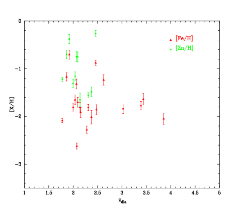
Figure 24.— [Zn/H] and [Fe/H] measurements from the full sample of damped Ly$\alpha$ systems vs. redshift.

5. METALLICITY

We now turn to examine the metallicity of our sample of damped systems. Given the debate on the presence of dust in the damped Ly$\alpha$ systems, we will consider both Zn/H and Fe/H. Figure 24 plots our complete sample of [Zn/H] and [Fe/H] measurements vs. redshift. The column density-weighted mean for Zn,

$$[<{\rm Zn/H}>]=\log{\sum_{i}{N({\rm Zn^{+}})}_{i}\over\sum_{i}{N({\rm H^{0}})}_{i}}-\log({\rm Zn/H})_{\odot}\;\;\;,$$ (2)

for our full sample is [$<$Zn/H$>$] = $-1.15\pm 0.15$ dex. This result confirms that of Pettini et al. (1997). For Fe, we find [$<$Fe/H$>$] = $-1.64\pm 0.11$ dex for $z<3$ and $-1.77\pm 0.11$ dex for $z>3$. Lu et al. (1997) have used similar measurements (in fact several of the values presented here) to conclude that $z\approx 3$ marks the onset of significant star formation in the damped Ly$\alpha$ systems. Their interpretation is based on the fact that the damped systems exhibit a break in [$<$Fe/H$>$] at $z\approx 3$. Formally, our data does not support their conclusion, but the fact that the high redshift [$<$Fe/H$>$] value is dominated by only three systems (Q0000$-$26, Q0019$-$15, and Q0347$-$38) suggests our result is probably suffering from small number statistics.

6. SUMMARY AND CONCLUSIONS

We have presented accurate ionic column density and abundance measurements for 19 damped Ly$\alpha$ systems observed with HIRES on the 10m W.M. Keck Telescope. Throughout the paper we have utilized the apparent column density techniques to analyze the damped Ly$\alpha$ profiles and have adopted ${N({\rm HI})}$ values from the literature. The main results of the paper are summarized as follows:

1. The abundance patterns of our 19 systems match those observed by Lu et al. (1996). Therefore, our analysis confirms their primary conclusion that the damped Ly$\alpha$ systems exhibit abundance patterns representative of Type II SN enrichment with the major exception of [Zn/Fe] and to a lesser extent [Ni/Fe]. The Zn and Ni patterns, however, are in accordance with what one would expect for dust depletion based on observations of the lightly depleted, ’warm’ HI clouds in the ISM. While the combination of dust depletion and Type II SN enrichment fits the majority of the observations, this interpretation is ruled out by the observed values of [S/Fe].

2. A majority of the damped Ly$\alpha$ elemental abundances are consistent with a dust depletion pattern on top of an underlying solar abundance pattern. Observations of Titanium and Manganese, however, strongly contradict this interpretation. In every system where Ti is observed, we measure [Ti/Fe] $\geq 0$ dex consistent with the observed overabundance found in metal-poor halo stars and therefore suggestive of Type II SN enrichment. Similarly, the observed underabundance of [Mn/Fe] (Lu et al. (1996)) is opposite to the effects of dust depletion and therefore requires a nucleosynthetic explanation, albeit not necessarily Type II SN yields.

3. Our metallicity measurements confirm the principal results from the surveys of Pettini and collaborators. Specifically, we find: [$<$Zn/H$>$] = $-1.15\pm 0.15$ dex, [$<$Fe/H$>$] = $-1.64\pm 0.11$ dex for $z<3$, and $-1.77\pm 0.11$ dex for $z>3$. Although we do not observe an evolution in the column density-weighted Fe abundance with redshift – as claimed by Lu et al. (1997) – we expect this inconsistency lies in the small number statistics of our high $z$ sample.

4. For a number of damped Ly$\alpha$ systems in our sample (e.g. Q1331, Q0201, Q2348), we observe metal-line systems within 500 ${\rm\;km\;s^{-1}}$ of the damped system. In the case of Q2348, for example, a metal-line system exhibiting SiII, SiIV and AlIII transitions is located only $100{\rm\;km\;s^{-1}}$ from the strongest damped Ly$\alpha$ component. The absence of FeII and OI absorption and the SiII/SiIV ratio for this component, however, indicates this system is significantly ionized. We believe the same is true for the majority of these neighboring metal-line systems (the system at $z=1.858$ toward Q2230$+$02 is a notable exception). If they were identified independently of the damped system, these systems would be very strong Lyman limit systems. Their coincidence with the damped system suggests they lie within the halo enclosing the damped system or perhaps that of a neighboring protogalactic system. We expect a detailed analysis of these systems may provide important insight into the physical conditions surrounding the damped Ly$\alpha$ systems.

Figure 2.— Velocity plot of the metal-line transitions for the damped Ly$\alpha$ system at $z=3.439$ toward Q0019$-$15. The vertical line at $v=0$ corresponds to $z=3.43866$.

Figure 3.— Velocity plot of the metal-line transitions for the damped Ly$\alpha$ system at $z=2.309$ toward Q0100$+$13. The vertical line at $v=0$ corresponds to $z=2.309$.

Figure 4.— Velocity plot of the metal-line transitions for the damped Ly$\alpha$ system at $z=2.141$ toward Q0149$+$33. The vertical line at $v=0$ corresponds to $z=2.140755$.

Figure 5.— Velocity plot of the metal-line transitions for the damped Ly$\alpha$ system at $z=3.025$ toward Q0347$-$38. The vertical line at $v=0$ corresponds to $z=3.0247$.

Figure 6.— Velocity plot of the metal-line transitions for the damped Ly$\alpha$ system at $z=2.040$ toward Q0458$-$02. The vertical line at $v=0$ corresponds to $z=2.03955$.

Figure 7.— Velocity plot of the metal-line transitions for the damped Ly$\alpha$ system at $z=2.374$ toward Q0841$+$12. The vertical line at $v=0$ corresponds to $z=2.374518$.

Figure 8.— Velocity plot of the metal-line transitions for the damped Ly$\alpha$ system at $z=2.476$ toward Q0841$+$12. The vertical line at $v=0$ corresponds to $z=2.476219$.

Figure 9.— Velocity plot of the metal-line transitions for the damped Ly$\alpha$ system at $z=3.386$ toward Q0951$-$04. The vertical line at $v=0$ corresponds to $z=3.856689$.

Figure 10.— Velocity plot of the metal-line transitions for the damped Ly$\alpha$ system at $z=4.203$ toward Q0951$-$04. The vertical line at $v=0$ corresponds to $z=4.202896$.

Figure 11.— Velocity plot of the metal-line transitions for the damped Ly$\alpha$ system at $z=1.999$ toward Q1215$+$33. The vertical line at $v=0$ corresponds to $z=1.9991$.

Figure 12.— Velocity plot of the metal-line transitions for the damped Ly$\alpha$ system at $z=1.776$ toward Q1331$+$17. The vertical line at $v=0$ corresponds to $z=1.77636$.

Figure 13.— Velocity plot of the metal-line transitions for the damped Ly$\alpha$ system at $z=3.736$ toward Q1346$-$03. The vertical line at $v=0$ corresponds to $z=3.735830$.

Figure 14.— Velocity plot of the metal-line transitions for the damped Ly$\alpha$ system at $z=2.625$ toward Q1759$+$75. The vertical line at $v=0$ corresponds to $z=2.6253$.

Figure 15.— Velocity plot of the metal-line transitions for the damped Ly$\alpha$ system at $z=1.864$ toward Q2230$+$02. The vertical line at $v=0$ corresponds to $z=1.864388$.

Figure 16.— Velocity plot of the metal-line transitions for the presumed damped system at $z=1.859$ toward Q2230$+$02. The vertical line at $v=0$ corresponds to $z=1.858536$.

Figure 17.— Velocity plot of the metal-line transitions for the damped Ly$\alpha$ system at $z=2.066$ toward Q2231$-$00. The vertical line at $v=0$ corresponds to $z=2.06615$.

Figure 18.— Velocity plot of the metal-line transitions for the damped Ly$\alpha$ system at $z=2.279$ toward Q2348$-$14. The vertical line at $v=0$ corresponds to $z=2.2794$.

Figure 19.— Ly$\alpha$ profile for the damped system toward Q2348$-$14. The overplotted curves correspond to ${N({\rm HI})}=20.56\pm 0.075$.

Figure 20.— Velocity plot of the metal-line transitions for the damped Ly$\alpha$ system at $z=2.095$ toward Q2359$-$02. The vertical line at $v=0$ corresponds to $z=2.095067$.

Figure 21.— Velocity plot of the metal-line transitions for the damped Ly$\alpha$ system at $z=2.154$ toward Q2359$-$02. The vertical line at $v=0$ corresponds to $z=2.153934$.

References

- Evardsson et al. (1993) Evardsson, B., Anderson, J., Gutasfsson, B., Lambert, D.L., Nissen, P.E., and Tompkin, J. 1993, Astronomy and Astrophysics, 275, 101.
- Fall & Pei (1993) Fall, S.M. & Pei, Y.C. 1993, ApJ, 402, 479
- Ferland (1991) Ferland, G. J. 1991, Ohio State Internal Report 91-01
- Hoffman et al. (1996) Hoffman, R.D. et al. 1996, ApJ, 460, 478
- Howk & Savage (1998) Howk, J.C. & Savage, B.D. 1998, ApJ, submitted
- Kulkarni et al. (1997) Kulkarni, V.P., Fall, S.M., & Truran, J.W. 1997, ApJ, 484, 7
- Lipman & Pettini (1995) Lipman, K. & Pettini, M. 1995, ApJ, 442, 628
- Lu et al. (1996) Lu, L., Sargent, W.L.W., Barlow, T.A., Churchill, C.W., & Vogt, S. 1996, ApJS, 107, 475
- Lu et al. (1997) Lu, L., Sargent, W.L.W., Barlow, T.A., 1997,
- Malaney and Chaboyer (1996) Malaney, R.A. and Chaboyer, B. 1996, ApJ, 462, 57
- McWilliam (1997) McWilliam, Andrew 1997, ARA&A, 35, 503
- Morton (1991) Morton, D.C. 1991, ApJS, 77, 119
- Nakamura et al. (1998) Nakamura, T., Umeda, H., Nomoto, K., Thielemann, F., & Burrows, A. 1998, ApJ, submitted (astro-ph/9809307)
- Pettini et al. (1994) Pettini, M., Smith, L. J., Hunstead, R. W., and King, D. L. 1994, ApJ, 426, 79
- Pettini et al. (1995) Pettini, M., Lipman, K., & Hunstead, R.W. 1995, ApJ, 451, 100
- Pettini et al. (1997) Pettini, M., Smith, L.J., King, D.L., & Hunstead, R.W. 1997, ApJ, 486, 665
- Pettini et al. (1998) Pettini, M., Ellison, S., Steidel, C.C., & Bowen, D.V. 1998, ApJ, in press
- Prochaska & Wolfe (1996) Prochaska, J. X. & Wolfe, A. M. 1996, ApJ, 470, 403
- (19) Prochaska, J. X. & Wolfe, A. M. 1997, ApJ, 474, 140
- (20) Prochaska, J. X. & Wolfe, A. M. 1997, ApJ, 486, 73
- Prochaska & Wolfe (1998) Prochaska, J. X. & Wolfe, A. M. 1998, ApJ, in press
- Savage and Sembach (1991) Savage, B. D. and Sembach, K. R. 1991, ApJ, 379, 245
- Savage and Sembach (1996) Savage, B. D. and Sembach, K. R. 1996, ARA&A, 34, 279
- Songaila et al. (1994) Songaila et al. 1994, Nature, 371, 43
- Sneden et al. (1991) Sneden, C., Gratton, R.G., & Crocker, D.A. 1991, A & A, 246, 354
- Storrie-Lombardi and Wolfe (1998) Storrie-Lombardi, L.J. & Wolfe, A.M. 1998, in preparation
- Tripp et al. (1996) Tripp, T. M., Lu L., & Savage B.D. 1996, ApJS, 102, 239
- Viegas (1994) Viegas, S.M. 1994, MNRAS, 276, 268
- Vladilo (1998) Vladilo, G. 1998, ApJ, 493, 583
- Vogt (1992) Vogt, S. S. 1992, in ESO Conf. and Workshop Proc. 40, High Resolution Spectroscopy with the VLT, ed. M.-H. Ulrich (Garching: ESO), p. 223
- Welty et al. (1997) Welty, D.E., Lauroesch, J.T., Blades, J.C., Hobbs, L.M., & York, D.G. 1997, ApJ, 489, 672
- Wolfe & Davis (1979) Wolfe, A.M., & Davis, M.M. 1979, AJ, 84, 699
- Wolfe et al. (1986) Wolfe, A.M., Turnshek, D.A., Smith, H.E., & Cohen, R.D. 1986, ApJS, 61, 249
- Wolfe et al. (1995) Wolfe, A. M., Lanzetta, K. M., Foltz, C. B., and Chaffee, F. H. 1995, ApJ, 454, 698
- Wolfe & Prochaska (1998) Wolfe, A.M. & Prochaska, J.X. 1998, ApJ, 494, 15L
- Zsarg & Federman (1998) Zsarg, J. & Federman, S.R. 1998, ApJ, 498, 256