Wavelet analysis and the detection of non-Gaussianity in the CMB

Abstract

We investigate the use of wavelet transforms in detecting and characterising non-Gaussian structure in maps of the cosmic microwave background (CMB). We apply the method to simulated maps of the Kaiser-Stebbins effect due to cosmic strings onto which Gaussian signals of varying amplitudes are superposed. We find the method significantly outperforms standard techniques based on measuring the moments of the pixel temperature distribution. We also compare the results with those obtained using techniques based on Minkowski functionals, and we again find the wavelet method to be superior. In particular, using the wavelet technique, we find that it is possible to detect non-Gaussianity even in the presence of a superposed Gaussian signal with five times the rms amplitude of the original cosmic string map. We also find that the wavelet technique is useful in characterising the angular scales at which the non-Gaussian signal occurs.

1 Introduction

The cosmic microwave background (CMB) is widely considered as one of the most important experimental tools in investigating the formation of structure in the Universe. In particular, by observing the temperature fluctuations in the CMB, we hope to distinguish between two competing theoretical paradigms. The first is the standard inflationary model, incorporating cold dark matter, for which the distribution of temperature fluctuations in the CMB should be Gaussian. The second class of theories invoke the formation of topological defects such as cosmic strings, monopoles or textures. In these theories the CMB temperature fluctuations are expected to be non-Gaussian, possessing steep gradients or well-defined ‘hot spots’ of emission (Bouchet, Bennett & Stebbins 1988; Turok 1996). Thus the detection (or otherwise) of a non-Gaussian signal in the CMB is an important means of discriminating between these two classes of theory.

Even in defect theories, however, it is possible that the non-Gaussian CMB signal may be obscured by an additional Gaussian component of primordial CMB fluctuations, by foreground emission from the Galaxy, or by instrumental noise. Moreover, CMB fluctuations arising from realistic defect cosmologies may well contain a Gaussian component that has a similar power spectrum to that of the non-Gaussian component (Magueijo & Lewin 1997), thereby making the task of detecting the non-Gaussian signal even more difficult. It is therefore important to investigate the regimes in which underlying non-Gaussianity can be detected when additional Gaussian signals are present. The most common technique is to define a statistic with properties that are easily calculated for Gaussian processes and then apply this statistic to the (possibly) non-Gaussian CMB map. In this way it is often possible to determine the probability that a given test map is drawn from an underlying Gaussian ensemble. Several approaches to this problem have already been proposed. Perhaps the most straightforward of these is the measurement of the skewness and kurtosis of the distribution of pixel temperatures in the map (Scaramella & Vittorio 1991). More elaborate methods include the calculation of the 3-point correlation function of the temperature distribution (Kogut et al. 1996) and the investigation of the statistics of maxima and minima in the map (Bond & Efstathiou 1987; Vittorio & Juskiewicz 1987). Methods based on the topological properties of the two-dimensional CMB temperature distribution have also been proposed (Coles 1988; Gott et al. 1990). The most recent of these techniques is based on the calculation of the three Minkowski functionals of the temperature distribution (see Section 5).

In this paper, we investigate the use of a new method for detecting non-Gaussianity which is based on the idea of expressing the CMB temperature distribution in terms of a set of two-dimensional wavelet basis functions (Fang & Pando 1996; Ferreira, Magueijo & Silk 1997). The wavelet transform provides a natural decomposition of the image into structure on different scales and, by analysing the distribution of wavelet coefficients on a given scale, it is possible to avoid the usual restrictions imposed by the central limit theorem, so that non-Gaussian signal is more easily detected. We apply this technique to simulated maps of the CMB that contain both a non-Gaussian contribution, due to the Kaiser-Stebbins effect from cosmic strings (Kaiser & Stebbins 1984), and also a Gaussian component with an identical power spectrum to the strings map. By varying the relative amplitudes of the two contributions, we determine to what extent the non-Gaussian signal can be obscured while still remaining detectable by the wavelet method. We compare our results with those obtained using either Minkowski functionals or straightforward calculation of the moments of the pixel temperature distribution.

2 The discrete wavelet transform

The discrete wavelet transform (DWT) has been discussed extensively elsewhere (e.g. Daubechies 1992). In particular, a characteristically clear introduction is given by Press et al. (1994). We therefore give only a brief description of its properties.

2.1 The one-dimensional DWT

It is best initially to discuss the DWT in just one dimension. In order to develop an intuitive understanding, let us begin by considering a periodic function $f(x)$ of period $L$ that we wish to expand in terms of a wavelet basis. The construction of the wavelet basis begins with the specification of the mother (or analysing) wavelet $\psi(x)$, together with another related function $\phi(x)$ called the father wavelet (or scaling function). In order to construct a wavelet basis that is discrete, orthogonal and compactly-supported, the functions $\phi(x)$ and $\psi(x)$ must together obey several highly-restrictive mathematical relations first derived by Daubechies (1992). We will not list these relations here, but merely note that the most straightforward requirements are that

$$\int_{-\infty}^{\infty}\phi(x)\,{\rm d}x = 1,$$ (1)

$$\int_{-\infty}^{\infty}\psi(x)\,{\rm d}x = 0.$$ (2)

Mother and father functions with compact support are usually defined on the interval $[0,1]$, and the wavelet basis is then constructed from dilations and translations of $\phi(x)$ and $\psi(x)$ as

$$\phi_{j,l}(x) = \left(\frac{2^{j}}{L}\right)^{1/2}\phi(2^{j}x/L-l),$$ (3)

$$\psi_{j,l}(x) = \left(\frac{2^{j}}{L}\right)^{1/2}\psi(2^{j}x/L-l),$$ (4)

where $j$ and $l$ are integers. The index $j$ labels the scale size of the wavelet, whereas $l$ labels the position of the wavelet at this scale. The set $\{\phi_{0,l},\psi_{j,l}\}$ with $0\leqslant j<\infty$ and $-\infty<l<\infty$ forms a complete, orthonormal basis in the space of functions of period $L$. The orthogonality of these functions is formally given by

$$\int_{-\infty}^{\infty}\phi_{j,l}(x)\phi_{j,l^{\prime}}(x)\,{\rm d}x = \delta_{ll^{\prime}},$$

$$\int_{-\infty}^{\infty}\phi_{j,l}(x)\psi_{j^{\prime},l^{\prime}}(x)\,{\rm d}x = \delta_{jj^{\prime}}\delta_{ll^{\prime}},$$

$$\int_{-\infty}^{\infty}\psi_{j,l}(x)\psi_{j^{\prime},l^{\prime}}(x)\,{\rm d}x = \delta_{jj^{\prime}}\delta_{ll^{\prime}}.$$

Using these orthogonality relationships, we may then write the function $f(x)$ as

$$f(x)=\sum_{l=-\infty}^{\infty}a_{0,l}\phi_{0,l}(x)+\sum_{j=0}^{\infty}\sum_{l=-\infty}^{\infty}b_{j,l}\psi_{j,l}(x),$$ (5)

where the wavelet coefficients $a_{0,l}$ and $b_{j,l}$ are given by

$$a_{0,l} = \int_{-\infty}^{\infty}f(x)\phi_{0,l}(x)\,{\rm d}x,$$ (6)

$$b_{j,l} = \int_{-\infty}^{\infty}f(x)\psi_{j,l}(x)\,{\rm d}x.$$ (7)

So far we have assumed our function $f(x)$ is defined for all values of $x$. In many applications, however, the function is in fact digitised (sampled) at $N=2^{J}$ equally-spaced points $x_{i}$. In this case, by analogy with the Discrete Fourier Transform (DFT) of a sampled function, (5) becomes

$$f(x_{i})=a_{0,0}\phi_{0,0}(x_{i})+\sum_{j=0}^{J-1}\sum_{l=0}^{2^{j}-1}b_{j,l}\psi_{j,l}(x_{i}),$$ (8)

and the integrals for the wavelets coefficents in (6) & (7) are replaced by the appropriate summations. If the mean of the function samples, $f(x_{i})$, is zero (as will be case in this paper), then $a_{0,0}=0$ and the function can be described entirely in terms of the wavelets $\psi_{j,l}$. As the scale index $j$ increases from 0 to $J-1$, the wavelets represent the structure of the function on increasingly smaller scales, with each scale a factor of 2 finer than the previous one. The index $l$ (which runs from 0 to $2^{j}-1$) denotes the position of the wavelet $\psi_{j,l}$ within the $j$th scale level.

If we collect the function samples $f_{i}=f(x_{i})$ in a column vector f (whose length $N$ must an integer power of 2), then (like the DFT) the DWT is a linear operation that transforms f into another vector $\widetilde{\textbf{{f}}}$ of the same length, which contains the wavelet coefficients of the (digitised) function. The action of the DWT can therefore be considered as the multiplication of the original vector by the $N\times N$ wavelet matrix W to give

$$\widetilde{\textbf{{f}}}={\textbf{{W}}f}.$$ (9)

Again like the DFT, the wavelet matrix W is orthogonal, so the inverse transformation can be performed straightforwardly using the transpose of W. Thus both the DFT and DWT can be considered as rotations from the original orthonormal basis vectors ${\textbf{{e}}}_{i}$ in signal space to some new orthonormal basis $\widetilde{\textbf{{e}}}_{i}$ ($i=1,\ldots,N$), with the transformed vector $\widetilde{\textbf{{f}}}$ containing the coefficients in this new basis.

The original basis vectors ${\textbf{{e}}}_{i}$ have unity as the $i$th element and the remaining elements equal to zero, and hence correspond to the ‘pixels’ in the original vector f. Therefore the original basis is the most localised basis possible in real space. For the DFT, the new basis vectors $\widetilde{\textbf{{e}}}_{i}$ are (digitised) complex exponentials and represent the opposite extreme, since they are completely non-local in real space but localised in frequency space. For the DWT, the new basis vectors are the wavelets, which enjoy the characteristic property of being reasonably localised both in real space and in frequency space, thus occupying an intermediate position between the original ‘delta-function’ basis and the Fourier basis of complex exponentials. Indeed, it is the simultaneous localisation of wavelets in both spaces that makes the DWT such a useful tool for analysing data in wide range of applications.

Since the wavelet basis $\widetilde{\textbf{{e}}}_{i}$ consists of (digitised) dilations and translations of the mother and father wavelets $\psi(x)$ and $\phi(x)$, we can obtain a different wavelet basis for each pair of these functions that obey the Daubechies conditions. Thus there exists an infinite number of possible wavelet transforms, with different wavelet bases making different trade-offs between how compactly they are localised in either real space or frequency space. In this paper, we will be concerned only with wavelet bases for which the wavelets are continuous and have compact support in either space (it is impossible for a function to have compact support in both spaces).

The implementation of the DWT is based on a pyramidal algortihm (Daubechies 1992; Press et al. 1994), and its speed is comparable to a Fast Fourier Transform. The calculation is arranged so that the transformed signal vector $\widetilde{\textbf{{f}}}={\textbf{{W}}f}$, containing the wavelet coefficients, takes the form

$$\widetilde{\textbf{{f}}}=(a_{0,0},b_{0,0},b_{1,0},b_{1,1},b_{2,0},b_{2,1},b_{2,2},b_{2,3},\ldots)^{\rm t}.$$

Thus the wavelet coefficients are placed in order of increasing scale index $j$ and, within a given scale, the $2^{j}$ coefficients are ordered with increasing position index $l$.

2.2 The two-dimensional DWT

The extension of the DWT to two-dimensional signals (or images) is straightforward and is usually performed by taking simple tensor products of the one-dimensional wavelet basis to produce a two-dimensional wavelet basis given by

$$\phi_{0,0;l_{1},l_{2}}(x,y) = \phi_{0,l_{1}}(x)\phi_{0,l_{2}}(y)$$

$$\zeta_{j_{1},0;l_{1},l_{2}}(x,y) = \psi_{j_{1},l_{1}}(x)\phi_{0,l_{2}}(y)$$

$$\xi_{0,j_{2};l_{1},l_{2}}(x,y) = \phi_{0,l_{1}}(x)\psi_{j_{2},l_{2}}(y)$$

$$\psi_{j_{1},j_{2};l_{1},l_{2}}(x,y) = \psi_{j_{1},l_{1}}(x)\psi_{j_{2},l_{2}}(y).$$

If the two-dimensional pixelised image has dimensions $2^{J_{1}}\times 2^{J_{2}}$ then by analogy with (8) we have $0\leqslant j_{1}\leqslant J_{1}-1$ and $0\leqslant l_{1}\leqslant 2^{j_{1}}-1$, and similarly for $j_{2}$ and $l_{2}$.

In this paper, will we be concerned with two-dimensional pixelised maps of temperature fluctuations in the CMB with dimensions $256\times 256$ (i.e. $J_{1}=J_{2}=8$). If we denote such an image by the matrix T, then the matrix of wavelet coefficients is given by

$$\widetilde{\textbf{{T}}}={\textbf{{W}}TW}^{\rm t},$$ (10)

where W is the wavelet matrix introduced in (9) and ${\textbf{{W}}}^{\rm t}$ is its transpose. The structure of the matrix $\widetilde{\textbf{{T}}}$ containing the wavelet coefficients is shown in Fig. 1, where the pixel numbers are plotted on a logarithmic scale.

Figure 1: The domains of the matrix $\widetilde{\textbf{{T}}}$ containing the coefficients of the two-dimensional wavelet transform. The italic numbers show the value of $k=2^{j_{1}}+2^{j_{2}}$ in each domain; see text for details.

We see that the matrix is partitioned into separate domains according to the scale indices $j_{1}$ and $j_{2}$ in the horizontal and vertical directions respectively. By analogy with the one-dimensional case, as $j_{1}$ increases the wavelets represent the horizontal structure in the image on increasingly smaller scales. Similarly, as $j_{2}$ increases the wavelets represent the increasingly fine scale vertical structure in the image. Thus domains that lie in the leading diagonal in Fig.1 (i.e. with $j_{1}=j_{2}$) contain coefficients of two-dimensional wavelets that represent the image at the same scale in the horizontal and vertical directions, whereas domains with $j_{1}\neq j_{2}$ contain coefficients of two-dimensional wavelets describing the image on different scales in the two directions.

Finally, we note that for the two-dimensional DFT it is common to denote the distance from the origin in Fourier space by $k$, which serves as a measure of inverse scale-length. In a two-dimensional DWT, it is also useful to define a similar quantity, but in this case $k$ is an integer variable given by $k=2^{j_{1}}+2^{j_{2}}$ which takes certain prescribed values between $k_{\rm min}=2$ and $k_{\rm max}=2^{J_{1}-1}+2^{J_{2}-1}$. In our application $J_{1}=J_{2}=8$ and so $k_{\rm max}=256$. By definition, the value of $k$ is constant within each of the domains shown in Fig.1. The values of $k$ in each domain are shown as the italic numbers in Fig. 1. We note that $k$ takes the same value for domains lying symmetrically on either side of the leading diagonal.

3 Detecting non-Gaussianity with the DWT

As mentioned above, let us denote our two-dimensional pixelised test map of temperature fluctuations in the CMB by the matrix T. If the test map is not drawn from a Gaussian ensemble, then we might hope to measure this non-Gaussianity directly from the histogram of the pixel temperatures, i.e. the histogram of the elements of the matrix T. Indeed, Scaramella & Vittorio (1991) use the skewness and kurtosis of the pixel temperature distribution as statistics for detecting non-Gaussianity in CMB images.

As noted by Fang & Pando (1996), however, methods based on statistics of the pixel temperature distribution can be unreliable in detecting non-Gaussianity, as a result of the central limit theorem. For example, if an image consists of numerous non-Gaussian processes on different scale lengths, then from the central limit theorem we would expect the probability distribution of the pixel temperatures to tend to a Gaussian as the number of processes increases.

In this paper, therefore, rather than analysing the distribution of the elements of T, we concentrate instead on the statistics of the wavelet coefficients, contained in the matrix $\widetilde{\textbf{{T}}}$. The wavelet transform provides a natural decomposition of the image into structure on different scales, and within each scale the wavelet basis functions are well-localised. Thus, by analysing the distribution of wavelet coefficients on a given scale, it is possible to avoid the restriction of the central limit theorem and any non-Gaussian signal on this scale is far more pronounced.

3.1 Statistics of wavelet coefficients

Referring to Fig. 1, it is useful to consider together all the wavelet coefficients that lie in domains sharing the same value of $k$. It is straightforward to show (and is intuitively reasonable) that if the input image T is (cyclically) translated or rotated, then wavelet coefficients sharing the same $k$-value are merely rearranged within the relevant domains. Thus any statistic based on the distribution of all wavelet coefficients sharing the same $k$-value is invariant to translations and rotations of the input image.

In order to describe the statisics of the wavelet coefficients of a given test image, we could (for each value of $k$ separately) calculate estimators of the moments $\hat{\nu}_{r}$ ($r=1,2,3,\ldots$), or central moments $\hat{\mu}_{r}$, of the distributions of its wavelet coefficients (see the Appendix). In this way, we obtain moment spectra $\hat{\nu}_{r}(k)$ (or central moment spectra $\hat{\mu}_{r}(k)$) for $r=1,2,3,\ldots$ which describe the (scale dependent) statistics of the wavelet coefficients. As discussed by Ferreira et al. (1997), however, a better approach is to describe the distribution of wavelet coefficients at each $k$-value in terms of its cumulants. Using unbiassed estimators of the cumulants based on $k$-statistics (see the Appendix), we thus calculate cumulant spectra $\hat{\kappa}_{r}(k)$ ($r=1,2,3,\ldots$) of the wavelet coefficients of the test image.

For a given test image T, the cumulant spectra of the corresponding wavelet coefficients have some useful properties. Firstly, let us suppose that T is drawn from a Gaussian ensemble. Since the wavelet transform can be considered merely an orthogonal rotation of the basis vectors in image space, it is straightforward to show that the wavelet coefficients at each value of $k$ are also drawn from a Gaussian distribution. Thus, for Gaussian test images, the expectation value of the estimated cumulant spectra $\hat{\kappa}_{r}(k)$ of the wavelet coefficients is zero for $r>2$ (see the Appendix). Secondly, let us consider a test image ${\textbf{{T}}}={\textbf{{T}}}_{1}+{\textbf{{T}}}_{2}$ that is the sum of two independent processes ${\textbf{{T}}}_{1}$ and ${\textbf{{T}}}_{1}$. Since the DWT is a linear operation, we thus have $\widetilde{\textbf{{T}}}=\widetilde{\textbf{{T}}}_{1}+\widetilde{\textbf{{T}}}_{2}$. Using the additive property of cumulants discussed in the Appendix, we therefore find that the $r$th cumulant spectrum $\hat{\kappa}_{r}(k)$ of the wavelet coefficients of T is simply the sum of the corresponding cumulant spectra of the wavelet coefficients of ${\textbf{{T}}}_{1}$ and ${\textbf{{T}}}_{2}$ taken separately. Of course, this argument can be extended to an arbitrary number of independent processes.

The cumulant spectra $\hat{\kappa}_{r}(k)$ ($r=1,2,3,\ldots$) form our basic test for non-Gaussianity. The procedure is as follows. We begin with some (possibly non-Gaussian) test image T and perform a wavelet transform to obtain the corresponding matrix of wavelet coefficients $\widetilde{\textbf{{T}}}$ given by (10). We then calculate the cumulant spectra $\hat{\kappa}_{r}(k)$ of these wavelet coefficients. Returning to the original test image T, we then create a large number (5000 say) of equivalent Gaussian realisations (EGR). Each EGR is created by Fourier transforming the original test image, randomising the phases of the complex Fourier coefficients, and inverse Fourier transforming the result. In the randomisation step, the phase of each Fourier coefficient is drawn at random from a uniform distribution in the range $[0,2\pi]$. Thus each EGR has exactly the same power spectrum as the original test image, but the pixel temperature distribution is drawn from a Gaussian ensemble. Each EGR is then analysed in exactly the same way as the original test image in order to obtain the cumulant spectra of its wavelet coefficients. Thus, after analysing all the EGRs, we obtain (for each value of $k$) approximate probability distributions of the cumulant estimators $\hat{\kappa}_{r}(k)$ for a Gaussian process with the same power spectrum as the original test map. By comparing these probability distributions with the cumuluant spectra of the original image, we thus obtain an estimate of the probability that the original image was drawn from a Gaussian ensemble. For $256\times 256$ images considered here, the entire analysis requires about 20 minutes CPU time on a Sparc Ultra workstation.

We note that, in two-dimensional applications it is usual to consider only the domains in Fig. 1 with $j_{1},j_{2}\geqslant 1$. The main reason is that the domains with $j_{1}=0$ or $j_{2}=0$ contain a mixture of coefficients of the three different two-dimensional wavelet bases $\phi_{0,0;l_{1},l_{2}}(x,y)$, $\zeta_{j_{1},0;l_{1},l_{2}}(x,y)$ and $\xi_{0,j_{2};l_{1},l_{2}}(x,y)$. Domains with $j_{1},j_{2}\geqslant 1$, however, contain only the coefficients $b_{j_{1},j_{2};l_{1},l_{2}}$ of the basis $\psi_{j_{1},j_{2};l_{1},l_{2}}(x,y)$ and, as a result, statistics based on the distribution of these wavelet coefficients are generally more informative. Therefore, for the remainder of this paper, we will restrict our attention to domains with $j_{1},j_{2}\geqslant 1$.

3.2 Choosing the wavelet basis

Our only remaining task is to choose the wavelet basis in which we wish to expand our CMB map. As mentioned above, in this paper we restrict ourselves to discrete, orthogonal, compactly-supported wavelet bases. Nevertheless, there are still an infinite number of such bases and so we will concentrate on only a small subset of commonly-used wavelet bases. Our wavelet ‘library’ consists of the following one-dimensional wavelet bases: Haar; Daubechies 4,6,12,20; Coiflet 2,3; Symmlet 6,8. Several of these wavelets are plotted and discussed by Graps (1995). We note that this library is in no way intended to be an exhaustive set of useful wavelets, but represents a fairly typical range of bases which could be employed. As mentioned above, in each case, the corresponding two-dimensional wavelet basis is formed by taking the tensor product of the one-dimensional basis.

Since each wavelet basis provides a different decompostion of the CMB test image, the resulting cumulant spectra will be different in each case. Indeed, depending on the structure present in the test image, some wavelet bases will be more powerful at detecting non-Gaussianity than others. Since the analysis discussed above requires the wavelet transform of a large number of EGR to be calculated, it would clearly be very time-consuming to perform this for every available wavelet basis. Therefore, for a given test image, we wish to find a quick method by which we can determine the wavelet basis that is most sensitive to any non-Gaussian structure present.

We begin by calculating the wavelet coefficients $b_{j_{1},j_{2};l_{2},l_{2}}$ of the single test map in each of the available bases, which requires only a couple of seconds of CPU time on a Sparc Ultra workstation. For each basis, we then define the ‘normalised’ wavelet coefficients at each value of $k$ by

$$p_{j_{1},j_{2};l_{2},l_{2}}=\frac{b^{2}_{j_{1},j_{2};l_{2},l_{2}}}{\sum_{j_{1},j_{2},l_{1},l_{2}}b^{2}_{j_{1},j_{2};l_{2},l_{2}}},$$

where, in the denominator, the sum on the scale indices $j_{1}$ and $j_{2}$ is for all values satisfying $2^{j_{1}}+2^{j_{2}}=k$ and the sum on position indices $l_{1}$ and $l_{2}$ corresponds to all wavelets coefficients lying within the relevant scale domains. Thus, for each value of $k$, the coefficients $p_{j_{1},j_{2};l_{2},l_{2}}$ have values between zero and unity and the sum of all the coefficients is equal to unity. We then calculate (a multiple of) the entropy of the normalised wavelet coefficients for each value of $k$,

$$S=-\frac{1}{\ln N}\sum_{j_{1},j_{2},l_{1},l_{2}}p_{j_{1},j_{2};l_{2},l_{2}}\ln p_{j_{1},j_{2};l_{2},l_{2}}$$

where again the sum extends over all wavelet coefficients sharing the $k$-value under consideration and $N$ is the total number of these coefficients. We also note that $\lim_{p\to 0}p\ln p=0$. The value of the sum lies between $0$ and $-\ln N$, and so we have normalised $S$ so that its value always lies between zero and unity. The entropy $S$ takes the value zero if one of the coefficients $p_{j_{1},j_{2};l_{2},l_{2}}$ equals unity and the rest are zero. At the other extreme, $S$ equals unity when all the coefficients are equal.

Now, if the original CMB map is Gaussian, then, as mentioned above, the distribution of wavelet coefficients at each $k$-value is also Gaussian. Furthermore, for a Gaussian CMB map with structure on a wide range of scales, we would expect that, at each scale $k$, all the wavelet basis functions would be required, with roughly equal amplitudes, in order to represent the image on that scale. Hence the entropy of the normalised wavelet coefficients should be close to its maximum value of unity. For a map with pronounced non-Gaussian features, however, this is not necessarily the case. If there exists a wavelet basis that resembles the non-Gaussian features in the map on some scale, then we might expect the original image to be well represented by fewer basis functions. In this case, many of the wavelet coefficients may be close to zero, with just a few large coefficients corresponding to the basis functions that best resemble the main features in the image. We would therefore expect a lower value for the entropy of the normalised wavelet coefficients. Thus, for each wavelet basis in our library, we calculate the entropy of the wavelet coefficients of the test image at each value of $k$. The optimal basis is then taken as that having the lowest entropy for any $k$-value. For each of the test maps discussed in the next Section, the Coiflet 2 wavelet basis was found to be optimal. In particular, the entropy of the wavelet coefficients was especially low for $k=66$, which, as we shall see below, is the angular scale on which a non-Gaussian signal is detected with the highest significance for each test map.

4 Application to simulated CMB maps

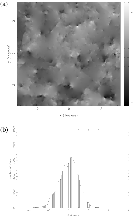
Figure 2: (a) A realisation of temperature fluctuations in the CMB due to the Kaiser-Stebbins effect from cosmic strings. The map is pixelised on a $256\times 256$ grid with a pixel size of 1.5 arcmin. For convenience the map has been normalised so that its variance equals unity. (b) A histogram of the pixel temperature distribution.

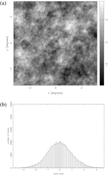
Figure 3: (a) A realisation of a Gaussian image with a power spectrum identical to that of the cosmic strings map shown in Fig. 2(a); see text for details. (b) A histogram of the pixel temperature distribution.

In this Section, we apply the wavelet transform technique described above to the detection of non-Gaussianity in simulated CMB maps. Our basic non-Gaussian test map is shown in Fig. 2(a) and is a realisation of CMB anisotropies due to the Kaiser-Stebbins effect from cosmic strings (Bouchet, Bennett & Stebbins 1988). The map is pixelised on a $256\times 256$ grid with a pixel size of 1.5 arcmin. Thus the size of the simulated field is $6.4\times 6.4$ deg². The map has zero mean and has, for convenience, been normalised so that its variance equals unity.

We see from Fig. 2(a) that the strings map is extremely non-Gaussian, possessing sharp temperature gradients and localised hot-spots. From the scale-bar, we also note that the maximum and minimum temperatures in the map are respectively $6.1$ and $-5.3$ times the rms value, again indicative of a highly non-Gaussian process. This non-Gaussianity is also apparent from the histogram of pixel temperatures shown in Fig. 2(b).

In order to assess to what extent the non-Gaussian signal in the strings map can be obscured, but still remain detectable, we will add to it some multiple of the Gaussian test map (GTM) shown in Fig. 3(a). The GTM shown is an equivalent Gaussian realisation of the cosmic strings map shown in Fig. 2(a) and thus has an identical power spectrum, but the pixel temperatures are drawn from a Gaussian distribution. Clearly, by construction, the GTM also has unit variance.

We could, of course, use a GTM that is not an equivalent Gaussian realisation of the strings map. For example, we could use a realisation of CMB fluctuations predicted from some inflationary model. Such a map would, however, in general possess a different power spectrum to the strings map and differences between the two could be discerned by measuring these different power spectra. By using a GTM that is an EGR of the strings map, we are considering the case of optimal confusion between the non-Gaussian and Gaussian signals and this should provide the most stringent test of the methods for detecting non-Gaussianity. Moreover, as mentioned in the Introduction, CMB fluctuations from realistic cosmic string cosmologies may well contain a Gaussian component that has a similar power spectrum to that of the non-Gaussian component. (Magueijo & Lewin 1997).

The differences between the strings map and the GTM are clear to the eye. The GTM possesses no sharp features or extreme maxima or minima. Furthermore, from the scale-bar, we see that the maximum and minimum of the pixel temperature distribution lie at 3.6 and -3.8 times the rms level, as one might expect for a Gaussian image with this number of pixels. The histogram of the pixel temperatures in the GTM is shown in Fig. 3(b) and is clearly closer to a Gaussian in shape than the corresponding histogram for the strings map shown in Fig. 2(b).

Our test maps thus consist of the sum of the above strings map and GTM in various proportions $(a:b)$. In order to make the simulations more realistic, before being analysed the test maps are first convolved with a 5-arcmin Gaussian beam and Gaussian pixel noise is added with an rms level equal to one-tenth that of the convolved map. This degree of smoothing and noise level is typical of what might be achieved for CMB observations using the ESA Planck Surveyor satellite (Bersanelli et al. 1996), after foreground contaminants have been removed using the maximum-entropy separation algorithm discussed by Hobson et al. (1998). The process of convolution smoothes out many of the sharp features visible in the underlying cosmic strings map in Fig. 2(a), and the addition of pixel noise obscures this structure still further. In each case, the resulting convolved, noisy test map is rescaled to have unit variance before being analysed for any non-Gaussian signal.

As mentioned above, for a wide range of non-Gaussian-to-Gaussian proportions $(a:b)$, the Coiflet 2 wavelet basis was found to be optimal for detecting the non-Gaussian signal due to the strings map in Fig.  2(a). Therefore, for the remainder of this paper, all wavelet decompositions will be in this basis. Furthermore, it was found, for our simulations, that the fourth cumulant spectrum, $\hat{\kappa}_{4}(k)$, was the most sensitive to the presence of any non-Gaussian signal, and so we will plot only this spectrum for each test map.

4.1 The Gaussian test map

We begin by assuming the CMB fluctuations to consist only of the Gaussian map shown in Fig. 3(a). Thus, formally, our initial test map consists of the sum of the cosmic strings map and the GTM in the proportions $(0:1)$ . This is then convolved with a 5-arcmin beam and pixel noise is added as discussed above. Applying the wavelet non-Gaussianity test to this image provides a useful check that a detection of non-Gaussianity is not obtained for a purely Gaussian signal. The resulting $\hat{\kappa}_{4}(k)$ cumulant spectrum of the wavelet coefficients of the test map is plotted as the solid squares in Fig. 4. As mentioned in Section 3.1, the same non-Gaussianity test is then also applied to 5000 equivalent Gaussian realisations (EGR) of the test map. In Fig. 4, the mean value of $\hat{\kappa}_{4}(k)$ obtained from the 5000 EGR is shown by the open circles, which all lie close to zero, as expected for a Gaussian process. At each value of $k$, the error bars show the 68, 95 and 99 per cent limits of the $\hat{\kappa}_{4}$ distribution obtained from the 5000 EGR. For presentational purposes, the cumulant spectrum has in fact been normalised so that, at each value of $k$, the variance of the $\hat{\kappa}_{4}$ distribution obtained from the 5000 EGR is equal to unity. Thus the significance of any detection of non-Gaussianity can be read off directly from the scale on the vertical axis of the plot. As might be expected in this case, however, the $\hat{\kappa}_{4}(k)$ spectrum of the test map lies well within the 2-sigma limits of the Gaussian ensemble at all values of $k$.

Figure 4: The $\hat{\kappa}_{4}(k)$ spectrum (solid squares) of the wavelet coefficients of the test map consisting of the sum of the cosmic strings map shown in Fig. 2(a) and the Gaussian test map shown in Fig. 3(a) in the proportions $(0:1)$, after convolution with a 5-arcmin Gaussian beam and the addition of Gaussian pixel noise with rms equal to one-tenth that of the convolved map. The open circles show the mean $\hat{\kappa}_{4}(k)$ spectrum obtained from 5000 equivalent Gaussian realisations of the test map (see text for details) and the error bars show the 68, 95 and 99 per cent limits of the resulting $\hat{\kappa}_{4}$ distribution at each value of $k$. For presentational purposes, the spectrum been normalised so that, at each value of $k$, the variance of the $\hat{\kappa}_{4}$ distribution obtained from the 5000 EGR is equal to unity. The point at $k=1$ is not calculated from the wavelet coefficients, but instead shows the values of $\hat{\kappa}_{4}$ obtained directly from the pixel temperature distributions in the test map and the 5000 EGR.

As discussed in Section 3.1, since we ignore domains of the wavelet transform with $j_{1}$ or $j_{2}$ equal to zero, we see from Fig. 1 that the $\hat{\kappa}_{4}(k)$ spectrum of the wavelet coefficients should start at $k=4$. The point plotted at $k=1$ in Fig. 4 is not in fact calculated from the wavelet coefficients, but instead shows the values of $\hat{\kappa}_{4}$ obtained directly from the pixel temperature distributions in the test map and the 5000 EGR. This point therefore represents a non-Gaussianity test similar to that proposed by Scaramella & Vittorio (1991), in which the skewness and kurtosis of the pixel temperature distributions were calculated. The point is included to provide an immediate comparison between methods based on the statistics of the wavelet coefficients and those based directly on the statistics of the pixel temperature distribution.

4.2 The cosmic strings map

Figure 5: As in Fig. 4, but for the test map with non-Gaussian: Gaussian proportions $(1:0)$.

We may repeat the above analysis for the opposite extreme in which the CMB fluctuations are assumed to consist only of the cosmic strings contribution (so that the non-Gaussian:Gaussian proportions are formally $(1:0)$). As before, the map is then convolved with a 5-arcmin beam and pixel noise is added. The resulting $\hat{\kappa}_{4}(k)$ spectrum is shown in Fig. 5. We see from the figure that unambiguous detections of non-Gaussianity are obtained at numerous values of $k$, the most spectacular being a 910-sigma detection at $k=66$. As discussed in Section 3.2, the entropy of the wavelet coefficients for the Coiflet 2 basis was lowest in the domains with $k=66$, and so we might have expected these domains to provide the most significant detection of non-Gaussianity.

Indeed, since the detection of non-Gaussianity is so large, it is not possible to discern the error bars denoting the confidence limits of the $\hat{\kappa}_{4}$ distributions for the 5000 EGR (although they are plotted). We merely note that for the $k=1$ point (calculated directly from the pixel temperatures), the significance of the non-Gaussian detection is only 1.1-sigma. Thus, in this case we find that, by analysing the wavelet coefficients of the image in separate $k$-domains, we obtain a vastly improved detection of non-Gaussianity as compared with analysing the pixel temperature distribution directly.

4.3 Mixed cosmic strings/Gaussian maps

Figure 6: As in Fig. 4, but for test maps with non-Gaussian: Gaussian proportions $(1:b)$.

Now we have analysed separately the cosmic strings map in Fig. 2(a) and the GTM in Fig. 3(a) (after convolution and the addition of pixel noise), we may repeat the analysis for test maps consisting of the sum of the cosmic strings map and GTM in different proportions $(1:b)$. It is clear that when $b\gg 1$ the resulting $\hat{\kappa}_{4}(k)$ spectrum of the wavelet coefficients will tend to that shown in Fig. 4. Similarly, if $b\ll 1$ the $\hat{\kappa}_{4}(k)$ spectrum will lie close to that in Fig. 5. In this Section, our aim is to find the value of $b$ at which the detection of non-Gaussianity becomes marginal. We reiterate that, in the following analysis, each test map is convolved and has noise added (as discussed above) before applying the non-Gaussianity test.

In Fig. 6 we plot the $\hat{\kappa}_{4}(k)$ spectra for test maps with $b=1,2,3,4,5,6$. We see from the figure that significant non-Gaussian detections are obtained for $b\leqslant 4$. We note that, in each case, the largest detection of non-Gaussianity occurs at $k=66$, as expected from the entropy analysis discussed in Section 3.2. The significance of the largest detections for $b=1,2,3,4$ is 495-, 88-, 24- and 9-sigma respectively. For $b=5$, the detection of non-Gaussianity becomes marginal. The largest signal again occurs at $k=66$, but the significance is only 4-sigma. For $b=6$, no detection is possible and, as expected, the $\hat{\kappa}_{4}(k)$ spectrum closely resembles that shown in Fig. 5 for the case when no non-Gaussian signal is present.

For all values of $b$, however, we note that for the $k=1$ point, which is calculated directly from the pixel temperatures, the value of $\hat{\kappa}_{4}$ for the test map lies within the 95 percent confidence limits of the of $\hat{\kappa}_{4}$ distribution obtained from the 5000 EGR. Thus, we see the statistic based on the pixel temperature distribution is far less sensitive to the presence of a non-Gaussian signal than those based on the wavelet coefficients of the image.

The performance of the wavelet non-Gaussianity test is encouraging. In particular, we must remember that the parameter $b$ represents the ratio of the rms values of the GTM and cosmic strings maps that constitute the test image. The ratio of the power in the Gaussian and non-Gaussian contributions is given by $b^{2}$ and so a marginal detection is still possible when the power due to the GTM is 25 times that due to the cosmic strings map. We note that, since the GTM possess an identical power spectrum to the cosmic strings map, the ratio of the power in the Gaussian and non-Gaussian contributions is equal to $b^{2}$ on all angular scales. Thus, the detection of non-Gaussianity is not the result of the presence of excess power in the cosmic strings map over some range of scales.

For illustration purposes, in Fig. 7(a) we plot the $b=5$ test map, after convolution and the addition of pixel noise. Although the wavelet non-Gaussianity test provided a marginal detection, as shown in Fig. 6(e), we see that, at least by eye, the non-Gaussian signal from the cosmic strings map in Fig. 2(a) is completely obscured by the signal due to the GTM in Fig. 3(a). Moreover, convolution with a 5-arcmin Gaussian beam and the addition of pixel noise have further diluted the non-Gaussian signal. The histogram is pixel temperatures is shown in Fig. 7(b) and is clearly close to Gaussian.

4.4 The cosmic strings map with enhanced pixel noise

As a final example, we consider again the case in which the CMB signal consists only of the cosmic strings map, convolved to 5-arcmin resolution (as in Section 4.2), but in which the level of instrumental pixel noise is increased such that its rms value is equal to that of the convolved CMB map. This example is included for two reasons. Firstly, it has traditionally been pixel noise that presented the greatest obstacle to the detection of non-Gaussianity in the CMB, and this is still the case for the 4-year COBE data. Although the observational strategy for our simulated data is very different from that used for the COBE observations, the information content of the two data-sets is comparable. The $6.4\times 6.4$ deg² map used here contains approximately 6000 5-arcmin beams, which is similar to the number of pixels in standard resolution COBE observations, although this somewhat larger than the number of independent COBE beams. The second reason for including this test image is to investigate the abilities of the wavelet technique when the main contaminant does not possess a power spectrum that is identical in shape to that of the non-Gaussian signal, but instead has a flat white-noise power spectrum.

The resulting $\hat{\kappa}_{4}(k)$ spectrum for this test map is shown in Fig. 8. We see from the figure that the most significant detection of non-Gaussianity is 42-sigma at $k=34$, accompanied by a 24-sigma detection at $k=66$ and several 5–10-sigma detections at other $k$-values. It is interesting to note that the most significant detection is much smaller than the 495-sigma detection obtained in Fig. 6(a) and occurs at a lower value of $k$. For Fig. 6(a), the main contaminant also had an rms equal to that of the cosmic strings map, but possessed an identical power spectrum. It is clear therefore that the wavelet technique is less effective at detecting the non-Gaussian signal due to the cosmic strings map when the main contaminant has a flat white-noise power spectrum. This is in fact to be expected, since the non-Gaussian signal in the strings map comes predominantly from sharp temperature gradients, which occur on small scales. As compared to the cosmic strings map, a pixel noise contaminant with the same rms value has relatively more power on small scales, and is therefore more effective at obscuring the non-Gaussian signal. By comparing Figs 6(a) and 8 more closely, this behaviour becomes more apparent. We see that in both cases a $\sim 40$-sigma detection is obtained at $k=34$, but the more significant detections in Fig. 6(a), which occur at higher $k$-values, have been much reduced in Fig. 8.

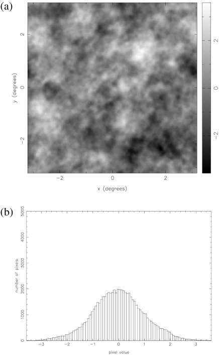
Figure 7: (a) The test map containing the cosmic strings map shown in Fig. 2(a) and the EGR shown on Fig. 3(a) in the proportions $(1:5)$. The map has been convolved with a 5-arcmin Gaussian beam and Gaussian pixel noise has been added with an rms equal to one-tenth that of the convolved CMB map. For convenience the map has been normalised to that its variance equals unity. (b) A histogram of the pixel temperature distribution.

Figure 8: As in Fig. 4, but for the test map with non-Gaussian: Gaussian proportions $(1:0)$ to which Gaussian pixel noise has been added with an rms value equal to that of the convolved CMB map.

5 Minkowski functionals analysis

In the previous Section, we found that the wavelet non-Gaussianity test was far more sensitive to the presence of a non-Gaussian signal than statistics based simply on the pixel temperature distribution of the CMB map. In order to compare the wavelet approach with other methods for detecting non-Gaussianity, in this Section we reanalyse the above test maps using an approach based on the topology of the CMB fluctuations.

The approach we adopt here requires the calculation of three Minkowski functionals for each test map. Minkowski functionals have been applied to CMB data in several forms previously. Schmalzing & Gorski (1998) derive the Minkowski functionals for a spherical sky and apply their results to the COBE four year data. Winitzki & Kosowsky (1998) give a detailed derivation of the expected form of the Minkowski functionals for a flat Euclidean space, taking into account boundary conditions, pixel noise and pixel size and shape. The reader is refered there for a more theoretical overview.

We opt here for an approach that is as simple as possible and use the three two-dimensional Minkowski functionals on square pixels in flat space. This approach is sufficient for the comparison desired in this paper. The three Minkowski functionals are the surface area, perimeter and Euler characteristic of an excursion region. The excursion region $R(T)$ is taken as the region of the map above a certain threshold temperature $T$, which is varied between the minimum and maximum values in the test map. The Minkowski functionals are therefore functions of the threshold temperature $T$. In two dimensions, the three functionals completely describe the statistical properties of a distribution. In terms of integral geometry they are given by

$$M_{0}(T) = \int_{R(T)}{\rm d}S,$$

$$M_{1}(T) = \int_{\partial R(T)}{\rm d}l,$$

$$M_{2}(T) = \int_{\partial R(T)}{{\rm d}l\over{r}}.$$

where $\partial R(T)$ is the boundary of the excursion region $R(T)$ at the threshold temperature $T$. The differentials ${\rm d}S$ and ${\rm d}l$ denote respectively the elements of area and of length along the boundary, and $r$ is the radius of curvature of the boundary. As an example, a circular disc of radius $a$ would have $M_{0}=\pi a^{2}$, $M_{1}=2\pi a$ and $M_{2}=2\pi$.

The surface area and perimeter of the excursion region in a pixelised map are trivial to calculate but the Euler characteristic requires a little explanation. It should be noted that, as defined here, the third Minkowski functional is equal to $2\pi G$ where $G$ is the genus of the excursion region. The genus is defined as the number of isolated holes (regions below the threshold) minus the number of islands (regions above the threshold) within the map. Using the approach advocated by Melott et al. (1989), based upon the three dimensional genus calculation of Hamilton, Gott & Weinberg (1986), we calculate the genus of the two-dimensional map by looking at the angle deficits of the vertices. Using this method it is also straightfoward to calculate the three Minkowski functionals simultaneously.

This approach to genus has been implemented previously and applied to the COBE data by Smoot et al. (1994), Kogut et al. (1996) and Colley, Gott & Park (1996). Gott et al. (1990) also looked at the use of the perimeter of the excursion regions but did not apply this analysis to any data. Theoretical predictions from defect theories have also been tested using the genus algorithm (see e.g. Avelino et al. (1998)) but the full Minkowski functional set is yet to be applied to a full CMB data set to constrain any cosmological parameters or defect theories. This has been carried out for various Large Scale Structure data sets (see e.g. Kerscher et al. 1997) with promising results.

5.1 Application to simulated CMB maps

Figure 9: Minkowski functionals analysis of the test map with non-Gaussian: Gaussian proportions $(1,0)$. Top panels: the three Minkowski functionals of the test map (dashed lines) calculated at 50 separate threshold temperatures between the minimum and maximum of the test map pixel temperature distribution. The solid lines show the mean Minkowski functionals calculated from 5000 EGR and the error bars denote the one-sigma limits of the probability distributions of the functionals at each temperature step. Bottom panels: the difference between the Minkowski functionals of the test map and mean Minkowski functionals of the 5000 EGR. At each temperature step, the plots have been normalised so that the one-sigma points of the probability distributions obtained from the 5000 EGR are equal to unity.

The three Minkowski functionals were calculated for the simulated CMB maps analysed in the previous Section. As discussed above, these test maps consist of the strings maps in Fig. 2(a) and the EGR in Fig 3(a) in proportions $(1:b)$, where $b$ can vary. Before being analysed, the test maps are first convolved with a 5-arcmin Gaussian beam and Gaussian pixel noise is added with an rms equal to one-tenth the rms of the convolved map. In each case the temperature range of the test map is divided into 50 steps and, at each temperature step, the three Minkowski functionals of the corresponding excursion region $R(T)$ are calculated. Following the procedure adopted in the wavelets non-Gaussianity test, in each case the three Minkowski functional are also calculated in an analogous manner for 5000 EGR so that approximate probability distributions are obtained for the values of the functionals at each temperature step.

Figure 10: As in Fig. 9, but for the test map with non-Gaussian: Gaussian proportions $(1:1)$.

Figure 11: As in Fig. 9, but for the test map with non-Gaussian: Gaussian proportions $(1:2)$.

Figure 12: As in Fig. 9, but for the test map with non-Gaussian: Gaussian proportions $(1:0)$ to which Gaussian pixel noise has been added with an rms value equal to that of the convolved CMB map.

The results for the cases $b=0$, 1 and 2 are shown in Figures 9–11. In the top three panels of each figure, we plot the Minkowski functionals of the test map (dashed lines) and the mean Minkowski functional for the 5000 EGR (solid lines). The error bars in each panel correspond to the one-sigma limits of the probability distributions of the values of the functionals at each temperature step, as obtained from the 5000 EGR. In order to estimate the significance of any non-Gaussian detection, in the bottom three panels of each figure we plot the difference between the Minkowski functionals of the test map and mean Minkowski functionals of the 5000 EGR. At each temperature step, the plots have been normalised so that the one-sigma points of the probability distributions obtained from the 5000 EGR are equal to unity. Thus, the significance of any non-Gaussian detection may be read-off directly from the vertical axis of each plot.

In the $b=0$ case (for which the test image is simply the convolved strings map with noise added), we see from the bottom three panels in Fig. 9 that significant detections of non-Gaussianity are obtained for all three Minkowski functionals. For low and high values of $T$, the corresponding excursions region of the test map are significantly different from those in a typical EGR and all three functionals detect some non-Gaussianity. Indeed the $M_{0}$, $M_{1}$ and $M_{2}$ functionals have detections of 14, 20 and 24-sigma respectively at high positive threshold temperatures. For the $M_{1}$ functional, we also see that, when the threshold temperature $T$ is close to zero (the mean of the maps), the excursion region $R(T)$ of the test map has a significantly smaller perimeter than for a typical EGR and a 6-sigma detection of non-Gaussianity is obtained.

This behaviour is easily understood by examining the structure present in the cosmic strings map shown in Fig. 2. The strings map possesses a great deal of structure for threshold temperatures near the minimum and maximum of the pixel temperature distribution. Even after convolution with the 5-arcmin beam, there still exist several sharply defined hot-spots and cold-spots that lie outside the typical 3-sigma range of the corresponding EGRs, and hence lead to large detections of non-Gaussianity. As noted earlier, the range of values in the (unconvolved) strings map is 6.1 to -5.3, and so at its extremes the temperature distribution is slightly skewed to positive values, which leads to more pronounced detections at high temperatures. Thus, as might be expected, the Minkowski functional analysis is powerful at detecting non-Gaussianity due to points in the strings map temperature distribution that lie outside the corresponding distribution of a typical EGR. For threshold temperatures near zero, however, the strings map is quite structureless, possessing large plane areas at constant temperature. Thus, the perimeter of a correpsonding excursion region will be quite small in comparison to an EGR and leads to the 6-sigma detection in the $M_{1}$ functional.

From Figs 10 & 11, however, we see that the results for $b=1$ and $b=2$ are somewhat disappointing. None of the Minkowski functionals have produced a significant detection of non-Gaussianity. Very few points lie outside the one-sigma limits obtained from the 5000 EGR and, even for $b=1$, the most significant deviation is only 2.5-sigma and must certainly not be considered as a robust detection of non-Gaussianity. Thus, we find that, in the presence of superposed Gaussian signals, the Minkowski functionals are far less sensitive than the wavelet technique to the presence of the non-Gaussian signal due to the cosmic strings map.

Finally, we perform the Minkowski functionals analysis on the enhanced noise map discussed in Section 4.4. The results are shown in Fig. 12. In contrast to the wavelets technique, we find that the Minkowski functionals are more sensitive to non-Gaussianity in the strings map when the main contaminant is pixel noise as opposed to an EGR. We see that the $M_{2}$ and $M_{3}$ functionals provide $\sim$8-sigma detections of non-Gaussianity at lower limit of the pixel temperature distribution.

6 Discussion and conclusions

We have investigated the use of wavelet analysis in detecting non-Gaussianity in the CMB. Our test images consist of non-Gaussian CMB fluctuations from the Kaiser-Stebbins effect due to cosmic strings plus some multiple of a Gaussian map with a power spectrum identical to the cosmic strings map. Before being analysed, the test images are convolved with a 5-arcmin Gaussian beam and Gaussian pixel noise is added with an rms equal to one-tenth that of the convolved test map. Using the wavelet technique, we find that the non-Gaussian signal can still be detected even when the superposed Gaussian map has an rms equal to 5 times that of the underlying cosmic strings map. However, statistics based directly on the pixel temperature distribution were unable to detect the non-Gaussian signal even in the absence of a superposed Gaussian map. The wavelet technique also produced clear detections of non-Gaussianity in the case where the cosmic strings map was contaminated by Gaussian pixel noise with the same rms value; in this regime standard methods were once again unsuccessful.

We also find that the wavelet technique outperforms methods based on the calculation of Minkowski functionals. Although the Minkowski functional approach yields a significant detection of non-Gaussianity for the case in which no Gaussian map is superposed, we find that, once a Gaussian signal with a equal rms value is added, no significant detection is obtained. However, the Minkowski functional technique did yield reasonable detections of non-Gaussianity in the high pixel noise regime. One possible way to improve the results from the Minkowski functional analysis may be to introduce into the method some notion of identifying localised structure, which is inherent in the wavelet technique. By looking at the distribution of Minkowski functionals as a function of position across the map it may be possible to make more significant detections of non-Gaussianity. Such a procedure has been investigated by Novikov, Feldman and Shandarin (1998), who use ‘partial’ Minkowski functionals to analyse the COBE 4-year data with promising results.

For both the wavelet and Minkowski functional analyses, we have quoted the significance of any detection of non-Gaussianity simply as the largest single deviation observed. This is, of course, the most conservative assumption that we can make, and corresponds to the situation in which a high degree of correlation exists bewteen the points in the $\hat{\kappa}_{4}(k)$ spectrum or between the values of the Minkowski functionals at different threshold temperatures. Thus, the significances quoted in this paper should properly be considered as lower limits. Clearly, if the points were independent, then we may simply multiply together the individual significances to obtain a greatly enhanced detection of non-Gaussianity. In order to obtain a value for the true level of significance for the wavelet or Minkowski functional approach, it is necessary to derive expressions for the correlations that exist between the individual points in each case. In particular, one would like to define some form of likelihood function that includes these correlations. We have not carried out such a procedure here, but will investigate these matters more fully in a forthcoming paper.

Finally, we mention how the current wavelet non-Gaussianity test might be further improved. The wavelet transform applied here decomposes the two-dimensional CMB temperature fluctuations into a two-dimensional wavelet basis. The bases used in this paper were constructed from the direct (tensor) product of existing commonly-used one-dimensional wavelet bases (see Section 2.2). The main disadvantage of this approach is the mixing of structure with different scales $j_{1}$ and $j_{2}$ in the horizontal and vertical directions. As pointed out by Mallat (1989), however, it is in fact possible to use one-dimensional wavelet bases to construct two-dimensional bases that do not mix scales and can be described in terms of a single scale index $j$. At each scale level $j$, these bases are given by

$$\phi_{j;l_{1},l_{2}}(x,y) = \phi_{j,l_{1}}(x)\phi_{j,l_{2}}(y)$$

$$\psi^{\rm H}_{j;l_{1},l_{2}}(x,y) = \psi_{j,l_{1}}(x)\phi_{j,l_{2}}(y)$$

$$\psi^{\rm V}_{j;l_{1},l_{2}}(x,y) = \phi_{j,l_{1}}(x)\psi_{j,l_{2}}(y)$$

$$\psi^{\rm D}_{j;l_{1},l_{2}}(x,y) = \psi_{j,l_{1}}(x)\psi_{j,l_{2}}(y).$$

The $\phi_{j;l_{1},l_{2}}$ wavelet is simply an averaging function at the $j$th level, while the other three wavelets correspond to structure at the $j$ scale level in the horizontal, vertical and diagonal directions in the image. Since such a basis does not mix structure on different scales, we might expect that it would provide wavelet decomposition of the CMB map that is more sensitive to the presence of any non-Gaussian signal. The application of this form of two-dimensional wavelet basis to the detection of non-Gaussianity in the CMB will be discussed in a forthcoming paper.

Even with the above modification, however, the wavelet non-Gaussianity test presented here is still restricted to flat two-dimensional images. Thus, in the context of the CMB, it can only be applied individually to small patches of sky for which the curvature of the sky is not significant. In order to apply the method to all-sky CMB maps, such as the COBE 4-year map or forthcoming maps from the MAP and Planck Surveyor missions, it is necessary to define two-dimensional wavelets on a sphere. A treatment of the continuous spherical wavelet transform and its discretization is given by Freeden & Winheuser (1996), and an algorithm for calculating bi-orthogonal discrete wavelet bases on a sphere is discussed by Schröder & Sweldens (1998). In addition to their possible use in detecting non-Gaussianity in all-sky CMB maps, the application of such wavelets to the general analysis of CMB data may also provide significant advantages in the compression of large data sets from the forthcoming MAP and Planck Surveyor satellite missions. These topics will also be investigated in a future paper.

Appendix A Moments, cumulants and k-statistics

For a detailed discussion of moments, cumulants and $k$-statistics the reader is referred to Struart & Ord (1994) or Kenney & Keeping (1954). Here, we outline only the basic definitions.

Let us consider the probability distribution $p(x)$ of some random variable $x$. The most straightforward description of $p(x)$ is in terms of its moments

$$\nu_{r}=\langle x^{r}\rangle,$$

where the angle brackets denote an ensemble average. Alternatively, one could describe the distribution using the central moments

$$\mu_{r}=\langle(x-\nu_{1})^{r}\rangle.$$

Clearly, if the mean $\nu_{1}$ of $p(x)$ is zero, then $\mu_{r}\equiv\nu_{r}$. The moments of a distribution are most conveniently described the its moment generating function (MGF), which is given by

$$M(h)\equiv\langle\exp(hx)\rangle=1+\nu_{1}h+\nu_{2}\frac{h^{2}}{2!}+\cdots+\nu_{r}\frac{h^{r}}{r!}+\cdots.$$ (11)

For example, the MGF of a Gaussian distribution with mean $\nu_{1}$ and variance $\sigma^{2}$ is

$$M(h)=\exp(\nu_{1}h+{\textstyle\frac{1}{2}}\sigma^{2}h^{2}).$$ (12)

Although the moments (or central moments) provide an intuitively straightforward description of the probability distribution $p(x)$, an alternative description in terms of its cumulants has several advantages. The cumulants $\kappa_{r}$ of $p(x)$ are defined through the cumulant generating function (CGF)

$$K(h)\equiv\ln M(h)\equiv\kappa_{1}h+\kappa_{2}\frac{h^{2}}{2!}+\cdots+\kappa_{r}\frac{h^{r}}{r!}+\cdots$$ (13)

By comparing (11) & (13), the cumulants of $p(x)$ are given in terms of its moments by (Stuart & Ord 1994)

$$\kappa_{r}=(-1)^{r-1}\left|\begin{array}[]{ccccc}\nu_{1}&\nu_{2}&\nu_{3}&\cdots&\nu_{r}\\ 1&\left({1\atop 0}\right)\nu_{1}&\left({2\atop 0}\right)\nu_{2}&\cdots&\left({r-1\atop 0}\right)\nu_{r-1}\\ 0&1&\left({2\atop 1}\right)\nu_{1}&\cdots&\left({r-1\atop 1}\right)\nu_{r-2}\\ 0&0&1&\cdots&\left({r-1\atop 2}\right)\nu_{r-3}\\ \vdots&\vdots&\vdots&&\vdots\\ 0&0&0&\cdots&\left({r-1\atop r-2}\right)\nu_{1}\end{array}\right|.$$ (14)

Evaluating this determinant for the first four cumulants, we find

$$\kappa_{1} = \nu_{1}$$

$$\kappa_{2} = \nu_{2}-\nu_{1}^{2}~{}=~{}\mu_{2}$$

$$\kappa_{3} = \nu_{3}-3\nu_{2}\nu_{1}+2\nu_{1}^{3}~{}=~{}\mu_{3}$$

$$\kappa_{4} = \nu_{4}-4\nu_{3}\nu_{1}+6\nu_{2}\nu_{1}^{2}-3\nu_{1}^{4}~{}=~{}\mu_{4}-3\mu_{2}^{2}.$$

There are clear advantages to using cumulants rather than moments to describe a probability distribution. Firstly, for two independent random variables $x$ and $y$, the cumulants are additive, i.e.

$$\kappa_{r}[x+y]=\kappa_{r}[x]+\kappa_{r}[y].$$

Secondly, from (12), we see that the CGF of a Gaussian distribution of mean $\nu_{1}$ and variance $\sigma^{2}$ is simply

$$K(h)=\nu_{1}h+{\textstyle\frac{1}{2}}\sigma^{2}h^{2}$$

Thus for a Gaussian distribution $\kappa_{r}=0$ for $r>2$.

From the cumulants and central moments, we can also define the dimensionless quantities

$$\chi_{r}=\kappa_{r}/\mu_{2}^{r/2}$$

of which $\chi_{3}$ and $\chi_{4}$ are better known as the skewness and kurtosis of the distribution. For a Gaussian distribution, $\chi_{3}=0$ and $\chi_{4}=3$, and so it is often useful to define the excess kurtosis ${\cal K}=\chi_{4}-3$, which equals zero for a Gaussian distribution.

Let us now consider a sample $x_{1},x_{2},\ldots,x_{N}$ of size $N$ drawn from the distribution $p(x)$. Clearly, these sample values may be used to obtain estimates of the cumulants of the parent distribution. The most straightforward method is first to estimate the moments or central moments of the distribution using

$$\hat{\nu}_{r} = \frac{1}{N}\sum_{i=1}^{N}x_{i}^{r},$$

$$\hat{\mu}_{r} = \frac{1}{N}\sum_{i=1}^{N}(x_{i}-\hat{\nu}_{1})^{r},$$

and then use (14) to obtain estimates $\hat{\kappa}_{r}$ of the cumulants. It is straightforward to show, however, that these estimates are biassed, so that $\langle\hat{\kappa}_{r}\rangle\neq\kappa_{r}$, and this bias is quite pronounced when the sample size $N$ is small. It is therefore better to estimate the cumulants of a distribution using $k$-statistics. The first four $k$-statistics are given by

$$\hat{\kappa}_{1} = \hat{\nu}_{1}$$

$$\hat{\kappa}_{2} = N\hat{\mu}_{2}/(N-1)$$

$$\hat{\kappa}_{3} = N^{2}\hat{\mu}_{3}/(N-1)(N-2)$$

$$\hat{\kappa}_{4} = N^{2}[(N+1)\hat{\mu}_{4}-3(N-1)\hat{\mu}_{2}^{2}]/(N-1)(N-2)(N-3).$$

The higher-order $k$-statistics are listed by Stuart & Ord (1994) up to $r=8$ but are extremely lengthy to write out in full. Using exact sampling theory, it is simple to show that these new estimators of the cumulants are unbiassed.

Finally, we note that, if the parent probability distribution $p(x)$ has zero mean, i.e. $\nu_{1}=0$ (as is the case for temperature fluctuations in the CMB), then there exists an alternative set of unbiassed estimators for the cumulants, which are much more straightforward to calculate. In this case, the first four estimators are given by

$$\hat{\kappa}_{1} = \hat{\nu}_{1}$$

$$\hat{\kappa}_{2} = \hat{\nu}_{2}$$

$$\hat{\kappa}_{3} = \hat{\nu}_{3}$$

$$\hat{\kappa}_{4} = [(N+2)\hat{\nu}_{4}-3N\hat{\nu}_{2}^{2}]/(N-1).$$

References

- [1] Avelino P.P., Shellard E.P.S., Wu J.H.P. & Allen B., astro-ph/9803120
- [2] Bersanelli M. et al., 1996, Report on Phase A Study for COBRAS/SAMBA, European Space Agency, Paris
- [3] Bond J.R., Efstathiou G., 1987, MNRAS, 226, 655
- [4] Bouchet F.R., Bennett D.P., Stebbins A., 1988, Nat, 335, 410
- [5] Coles P., 1988, MNRAS, 234, 509
- [6] Colley W.N., Gott III J.R., Park C. 1996, MNRAS, 281, L82
- [7] Daubechie I., 1992, Ten Lectures on Wavelets. S.I.A.M., Philadelphia
- [8] Fang L.Z., Pando J., 1996, in Sanchez N., Zichichi A., eds, Proc. International School of Astrophysics ‘D. Chalonge’, 5th Course: Current Topics in Astrofundamental Physics. World Scientific, Singapore, p. 616
- [9] Ferreira P.G., Magueijo J., Silk J., 1997, Phys. Rev. D, 56, 4592
- [10] Freeden W., Windheuser U., 1996, Adv. Comp. Math., 5, 51
- [11] Gott III J.R., Park C., Juszkiewicz R., Bies W., Bennett D.P., Bouchet F.R., Stebbins A., 1990, ApJ, 352, 1
- [12] Graps A.L., 1995, IEEE Comp. Sci. and Eng., 2, 50
- [13] Hamilton A.J.S., Gott III J.R., Weinberg D., 1986, ApJ, 309, 1
- [14] Hobson M.P., Jones A.W., Lasenby A.N., Bouchet F.R., 1998, MNRAS, in press
- [15] Kaiser N., Stebbins A., 1984, Nat, 310, 391
- [16] Kenney J.F., Keeping E.S., 1954, Mathematics of Statistics (Part I). Van Nostrand, New York
- [17] Kerscher M. et al., 1997, MNRAS, 284, 73
- [18] Kogut A., Banday A.J., Bennett C.L., Gorski K.M., Hinshaw G., Smoot G.F., Wright E.L., 1996, ApJ, 464, L29
- [19] Magueijo J., Lewin A., 1997, astro-ph/9702131
- [20] Mallat S.G., 1989, IEEE Trans. Acoust. Speech Sig. Proc., 37, 2091
- [21] Melott A.L., Cohen A.P., Hamilton A.J.S., Gott III J.R., Weinberg D., 1989, ApJ, 345, 618
- [22] Novikov D., Feldman H.A., Shandarin S.F., 1998, ApJ, submitted (astro-ph/9809238)
- [23] Press P.H., Teukolsky S.A., Vettering W.T., Flannery B.P., 1994, Numerical Recipes. Cambridge University Press, Cambridge
- [24] Scaramella R., Vittorio N., 1991, ApJ, 375, 439
- [25] Schmalzing J., Gorski K.M., 1998, MNRAS, in press (astro-ph/9710185)
- [26] Schröder P., Sweldens W., 1998, University of South Carolina, preprint
- [27] Smoot G.F., Tenorio L., Banday A.J., Kogut A., Wright W.L., Hinshaw G., Bennett C.L., 1994, ApJ, 437, 1
- [28] Stuart A., Ord K.J., 1994, Kendall’s Advanced Theory of Statistics (Volume I). Edward Arnold, London
- [29] Turok N., 1996, ApJ, 473, L5
- [30] Vittorio N., Juskiewicz R., 1987, ApJ, 314, L29
- [31] Winitzki S., Kosowsky A., 1998, New Astronomy, submitted (astro-ph/9710164)