Clustering in the ESP Redshift Survey

Abstract

ABSTRACT. We discuss the two-point correlation properties of galaxies in the ESO Slice Project (ESP) redshift survey, both in redshift and real space. The redshift-space correlation function $\xi(s)$ for the whole magnitude-limited survey is well described by a power law with $\gamma\sim 1.55$ between 3 and $\sim 40\rm\,h^{-1}\,Mpc$, where it smoothly breaks down, crossing the zero value on scales as large as $\sim 80\rm\,h^{-1}\,Mpc$. On smaller scales ($0.2-2\rm\,h^{-1}\,Mpc$), the slope is shallower mostly due to redshift-space depression by virialized structures, which are found to be enhanced by the J3 optimal-weighting technique. We explicitly evidence these effects by computing $\xi(r_{p},\pi)$ and the projected function $w_{p}(r_{p})$ . In this way we recover the real-space correlation function $\xi(r)$ , which we fit below $10\rm\,h^{-1}\,Mpc$ with a power-law model. This gives a reasonable fit, with $r_{o}=4.15^{+0.20}_{-0.21}h^{-1}\,$ Mpc and $\gamma=1.67^{+0.07}_{-0.09}$. This results on $\xi(r)$ and $\xi(s)$ and the comparison with other surveys clearly confirm how the shape of spatial correlations above $\sim 3\rm\,h^{-1}\,Mpc$ is characterised by a significant ‘shoulder’ with respect to the small-scale $\sim-1.8$ power law, corresponding to a steepening of P(k) near the turnover.

ABSTRACT. We discuss the two-point correlation properties of galaxies in the ESO Slice Project (ESP) redshift survey, both in redshift and real space. The redshift-space correlation function $\xi(s)$ for the whole magnitude-limited survey is well described by a power law with $\gamma\sim 1.55$ between 3 and $\sim 40\rm\,h^{-1}\,Mpc$, where it smoothly breaks down, crossing the zero value on scales as large as $\sim 80\rm\,h^{-1}\,Mpc$. On smaller scales ($0.2-2\rm\,h^{-1}\,Mpc$), the slope is shallower mostly due to redshift-space depression by virialized structures, which are found to be enhanced by the J3 optimal-weighting technique. We explicitly evidence these effects by computing $\xi(r_{p},\pi)$ and the projected function $w_{p}(r_{p})$ . In this way we recover the real-space correlation function $\xi(r)$ , which we fit below $10\rm\,h^{-1}\,Mpc$ with a power-law model. This gives a reasonable fit, with $r_{o}=4.15^{+0.20}_{-0.21}h^{-1}\,$ Mpc and $\gamma=1.67^{+0.07}_{-0.09}$. This results on $\xi(r)$ and $\xi(s)$ and the comparison with other surveys clearly confirm how the shape of spatial correlations above $\sim 3\rm\,h^{-1}\,Mpc$ is characterised by a significant ‘shoulder’ with respect to the small-scale $\sim-1.8$ power law, corresponding to a steepening of P(k) near the turnover.

1 Introduction

One of original goals of the ESO Slice Project (ESP) redshift survey was to study the clustering of galaxies from a survey hopefully not dominated by a single major superstructure (as it was the case for the surveys available at the beginning of this decade), being able to gather sufficient signal in the weak clustering regime, i.e. on scales above $10\rm\,h^{-1}\,Mpc$. After completion of the redshift survey, our first analyses concentrated on the galaxy luminosity function (the other main original goal), for which the ESP has yielded an estimate with unprecedented dynamic range (Zucca et al. 1997, Z97 hereafter). Here we shall report on the more recent results we have obtained on the clustering of ESP galaxies. The ESP covers a strip of sky $1^{\circ}$ thick (DEC) by $\sim 30^{\circ}$ long (RA) (with an unobserved $5^{\circ}$ sector inside this strip), in the SGP region. The target galaxies were selected from the EDSGC (Heydon-Dumbleton et al. 1989), and the final catalogue contains 3342 redshifts, corresponding to a completeness of 85% at a magnitude limit $b_{J}=19.4$. More details can be found in Vettolani et al. (1998). For the present analysis, we use comoving distances computed within a model with $H_{o}=100\mbox{km s${}^{-1}$}$ Mpc^-1 and $q_{o}=0.5$, while magnitudes are K-corrected as described in Z97.

2 Redshift-Space Correlations

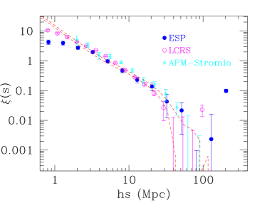
Figure 1: The redshift-space correlation function from the whole ESP magnitude-limited catalogue, compared to $\xi(s)$ from the LCRS and APM-Stromlo surveys. The dashed lines show the real space correlation function $\xi(r)$ derived from the APM $w(\theta)$, for two different clustering evolution models.

2.1 Optimal Weighting

The filled circles in Figure 1 show $\xi(s)$ computed from the whole ESP magnitude-limited sample using the J3-weighting technique (Guzzo et al. 1998, G98 hereafter). Note the smooth decay from the power law at large separations, with correlations going to zero only around $80\rm\,h^{-1}\,Mpc$, and perhaps some evidence for a positive fluctuation around $\sim 200\rm\,h^{-1}\,Mpc$. For $r<3\rm\,h^{-1}\,Mpc$, $\xi(s)$ tends to flatten (see below for more discussion on this). In the same figure, we reproduce $\xi(s)$ from the Las Campanas (LCRS, Tucker et al. 1997), and APM-Stromlo (Loveday et al. 1992), redshift surveys. There is a rather good agreement of the three independent data sets between 2 and $20\rm\,h^{-1}\,Mpc$, where $\xi(s)=(s/s_{\circ})^{-\gamma}$, with $s_{\circ}\sim 6\rm\,h^{-1}\,Mpc$ and $\gamma\sim 1.5$, with perhaps a hint for more power on larger scales in the blue-selected ESP and APM-Stromlo. In addition, the dashed lines describe the real-space $\xi(r)$ obtained by de-projecting the angular correlation function $w(\theta)$ of the APM Galaxy Catalogue (Baugh 1996), for two different assumptions on the evolution of clustering. It is rather interesting to note the degree of unanimity (within the error bars), between the angular and redshift data concerning the large-scale shape and zero-crossing scale ($40-90\rm\,h^{-1}\,Mpc$) of galaxy correlations. In fact, if one ideally extrapolates to larger scales the $\sim-1.8$ slope observed in real space below $3-4\rm\,h^{-1}\,Mpc$ [e.g. from the APM $\xi(r)$ ], all surveys agree in being consistently above this extrapolation, displaying what has been called a ‘shoulder’ or a ‘bump’ before breaking down (e.g. Guzzo et al. 1991). This excess power (see Peacock, these proceedings), requires in Fourier space a rather steep slope ($\sim k^{-2}$) for the power spectrum P(k). Such a feature is for example common in CDM models with an additional hot component (Bonometto & Pierpaoli 1998), or with high baryonic content (Eisenstein et al. 1998). On a different ground, the small amplitude difference between the redshift- and real-space correlations on scales $>5\rm\,h^{-1}\,Mpc$ is also remarkable, because implies a small amplification of $\xi(s)$ due to streaming flows, suggestive of a low value of $\beta=\Omega_{o}/b$.

2.2 Volume-limited estimates

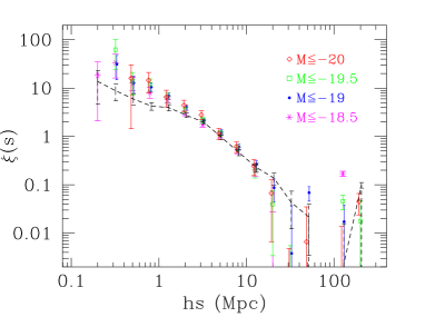
Figure 2: Redshift space correlation function for four volume-limited subsamples of the ESP survey, compared (dashed line with error bars) to the J3-weighted optimal estimate from the whole sample. For clarity, points for $M\leq-20$ and $M\leq-19$ are displayed with a constant shift in log(s).

While the J3-weighted estimate has the advantage of maximising the information extracted from the available data, it has a few drawbacks. The main one is that of mixing galaxy luminosities in the estimate of $\xi(s)$ . The worst aspect of this mixing is that it depends on scale: in fact, by its own definition, the method weighs pairs depending both on their separation and on their distance from the observer (see G98 for details).

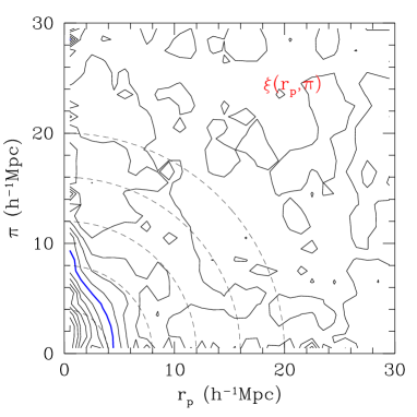
Figure 3: The $\xi(r_{p},\pi)$ map for the whole ESP survey, compared to the isotropic correlations expected in the absence of peculiar velocities (dashed). The heavy contour corresponds to $\xi=1$.

As a consequence, the main contribution to small-scale correlations comes from low-luminosity pairs, that are numerous in the nearer part of the sample, while $\xi(s)$ on large scales is mostly the result of correlations among high-luminosity objects, that are the in fact the only ones visible out to the more distant regions of the sample. Clearly, if there is any luminosity dependence of clustering, this technique will modify in some way the shape of $\xi(s)$ . In particular, if luminous galaxies are more clustered than faint ones, the J3 weighting will tend to produce a flatter estimate of $\xi(s)$ . In some way, therefore, while this method is certainly optimal for maximising the clustering signal on large scales (and so the previous discussion is certainly valid), it might be dangerous to draw from it conclusions on the global shape of $\xi(s)$ from, say, $0.1$ to $100\rm\,h^{-1}\,Mpc$. A wise way to counter-check the results produced using the optimal weighting technique, is that of estimating $\xi(s)$ also from volume-limited subsamples extracted from the survey. In this case, each sample includes a narrower range of luminosities, and no weighting is required, the density of objects being the same everywhere. We have performed this exercise on the ESP, selecting four volume-limited samples. The result is quite illuminating and is shown in Figure 2, directly compared to the J3-weighted estimate (dashed line). One can see that in fact at least in the case of our data, the latter method produces a $\xi(s)$ which is shallower below $\sim 3\rm\,h^{-1}\,Mpc$. Note, however, how on larger scales the shape is consistent between the two methods, and for $r>20\rm\,h^{-1}\,Mpc$ the J3 technique performs much better in terms of signal-to-noise, than the single volume-limited samples. By studying the distortions of $\xi(r_{p},\pi)$ and its projections (see below), we have seen that this small-scale redshift-space shape of the J3 estimate arises from a combination of a smaller real-space clustering and a larger pairwise velocity dispersion (see G98). Finally, from this figure one cannot notice any explicit dependence of clustering on luminosity, within the magnitude range considered. We shall see in the next section how this will change when we explore correlations free of redshift-space distortions.

3 $\xi(r_{p},\pi)$ and Real-Space
Correlations

More can be learned from redshift survey data, if we are able to disentangle the effect of clustering from that of the small-scale dynamics of galaxies, which adds to the Hubble flow to produce the observed redshift. This is traditionally done through the function $\xi(r_{p},\pi)$ (see e.g. G98), that essentially describes galaxy correlations as a function of two variables, one perpendicular ($r_{p}$), and the other parallel ($\pi$), to a sort of mean line of sight defined for each galaxy pair. In Figure 3, we show $\xi(r_{p},\pi)$ computed for the whole ESP survey, using the same technique used for $\xi(s)$. From this figure, one can clearly see the small-scale stretching of the contours along $\pi$, produced by the relative velocity dispersion of pairs within clusters and groups. Projecting $\xi(r_{p},\pi)$ onto the $r_{p}$ axis, one gets

$$w_{p}(r_{p}) \equiv 2\int_{0}^{\infty}dy\,\xi(r_{p},\pi)$$ (1)

$$= 2\int_{0}^{\infty}dy\,\xi\left(r\right)\,,$$

where now $\xi(r)$ is the real-space correlation function, with $r=\sqrt{r_{p}^{2}+y^{2}}$. $w_{p}(r_{p})$ is therefore independent from the redshift-distortion field, and is analytically integrable in the case of a power-law $\xi(r)=(r/r_{0})^{-\gamma}$. Given this form, the values of $r_{o}$ and $\gamma$ that best reproduce the data can be evaluated through an appropriate best-fitting procedure (G98). By applying this to the map of Figure 3, we recover $r_{o}=4.15^{+0.20}_{-0.21}h^{-1}\,$ Mpc and $\gamma=1.67^{+0.07}_{-0.09}$. As we anticipated in the previous section, this value of $r_{o}$ is slightly smaller than the value $\sim 5\rm\,h^{-1}\,Mpc$ which is measured by most other surveys, as e.g. the LCRS, and is an indication that our J3-weighted estimate on small scales could be biased in a subtle way towards faint, less clustered galaxies. In fact, while on one side the weighting scheme certainly amplifies the small-scale pairwise dispersion ($\sigma_{v}(1)\simeq 650\;\mbox{km s${}^{-1}$}$ with respect to $\sim 380\;\mbox{km s${}^{-1}$}$ measured from the $M\leq-20$ volume-limited sample), at the same time the contribution in projection from cluster galaxies seems to be still relatively low. This is in fact reasonable, given the small volume of the ESP ($\sim 1.9\cdot 10^{5}{\rm\,h^{-3}\,Mpc^{3}}$ at the effective depth of the survey.)

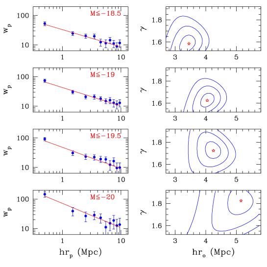
Figure 4: Best-fit results of a power-law $\xi(r)$ to the projected function $w_{p}(r_{p})$ for the four volume-limited samples.

Finally, we have computed $\xi(r_{p},\pi)$ and $w_{p}(r_{p})$ for the four volume-limited subsamples introduced in § 2.2. Figure 4 shows the result of the power-law fits to $w_{p}(r_{p})$ . A weak, but significant growth of $r_{\circ}$ and $\gamma$ with luminosity, especially for $M<M^{*}\simeq-19.5$, is evident. This is in contrast with the conclusions one could have drawn from the behaviour of $\xi(s)$ in Figure 2. The reason for this lays in the growing amount of small-scale redshift-space distortion in the four samples, that counter-balances the growth of clustering.

References

- [1] Bonometto, S.A., & Pierpaoli, E., 1998, NA, 3, 391
- [2] Baugh, C.M., 1996, MNRAS, 280, 267
- [3] Fisher, K.B., Davis, M., Strauss, M.A., Yahil, A., & Huchra, J.P. 1994a, MNRAS, 266, 50 (F94a)
- [4] Eisenstein, D., Hu, W., Silk, J., & Szalay, A.S., 1998, ApJ, 494, L1
- [5] Guzzo, L., Strauss, M.A., Fisher, K.B., Giovanelli, R., and Haynes, M.P. 1997, ApJ,, 489, 37
- [6] Guzzo, L., & the ESP Team, 1998, A&A,, submitted
- [7] Heydon-Dumbleton, N.H., Collins, C.A., MacGillivray, H.T., 1989, MNRAS, 238, 379
- [8] Loveday, J., Efstathiou, G., Peterson, B. A. Maddox, S. J., 1992, ApJ, 400, 43L
- [9] Tucker, D.L., Oemler, A., Kirshner, R.P., et al., 1997, MNRAS, 285, L5
- [10] Vettolani, G., & the ESP Team, 1997, A&A, 325, 954
- [11] Vettolani, G., & the ESP Team, 1998, A&AS, 130, 323
- [12] Zucca, E., & the ESP Team, 1997, A&A, 326, 477