Microwave background anisotropies and non-linear structures  II. Numerical computations

Abstract

A new method for modelling spherically symmetric inhomogeneities is applied to the formation of clusters in an expanding Universe. We impose simple initial velocity and density perturbations of finite extent and we investigate the subsequent evolution of the density field. Photon paths are also calculated, allowing a detailed consideration of gravitational lensing effects and microwave background anisotropies induced by the cluster. We apply the method to modelling high-redshift clusters and, in particular, we consider the reported microwave decrement observed towards the quasar pair PC1643+4631 A&B. We also consider the effect on the primordial microwave background power spectrum due to gravitational lensing by a population of massive high-redshift clusters.

1 Introduction

Several methods have been proposed for modelling the formation of galaxy clusters in an expanding Universe. Ideally, one would like to model the evolution of arbitrary matter perturbations in a fully general-relativistic manner. Unfortunately, this has not proved possible owing to the complication of the calculations involved, and models of the formation of clusters of arbitrary shape employ an approximate linearised approach to incorporate the effects of gravity (Martínez-González, Sanz & Silk 1990; Martínez-González & Sanz 1990; Chodorowski 1991). Nevertheless, many galaxy clusters can be reasonably approximated as ellipsoids, and some examples, such as the Coma cluster, are quasi-spherical. This naturally leads to the use of spherical symmetry as an approximation, which greatly reduces the computational complexity and allows the full incorporation of general-relativistic effects. Early approaches to this problem were based on the ‘Swiss Cheese’ model (Rees & Sciama 1968; Dyer 1976; Kaiser 1982; Nottale 1982 & 1984), whereas more recent attempts have used the continuous Tolman-Bondi solution (Panek 1992; Arnau et al. 1993; Sáez, Arnau & Fullana 1993; Arnau, Fullana & Sáez 1994; Fullana, Sáez & Arnau 1994; Quilis & Sáez 1998).

The Swiss Cheese and Tolman-Bondi approaches both assume that the cosmological fluid is pressureless. This assumption may be reasonable for very large structures in which the baryon content is negligible compared to the dark matter. For typical clusters, however, the assumption is perhaps questionable since 10–30 percent of the mass of the cluster may comprise a hot baryon component, with a non-negligible pressure, that is gravitationally coupled to the dark matter. Nevertheless, calculations by Quilis, Ibáñez & Sáez (1995), that include a hot gas component, show that the effects of pressure are in fact negligible, and that the collapse of the cluster is well approximated by assuming a pressureless fluid. However, the combined use of spherical symmetry and pressureless assumptions lead inevitably to the unrealistic situation where the cluster collapses to form a singularity. Therefore, for the applications described in this paper, we demand the density profile to be realistic at the time photons observed today are traversing the cluster. As pointed out by Quilis et al. (1995), the assumption of spherical symmetry introduces another difficulty. As a result of the radial structure of the velocity field, gravitational forces generate infalling motions that are too rapid and lead to fast evolution of the cluster, even when a hot gas component is included. An important consequence of this effect is that estimates of cosmic microwave background (CMB) anisotropies due to the cluster are overestimated and should be regarded as upper limits. However, for high redshift clusters still in the process of formation, such infalling motions may be less unrealistic (Navarro, Frenk & White 1996).

With these points in mind, in this paper we apply a new method for modelling the evolution of spherically symmetric anisotropies in the Universe, assuming a pressureless fluid. This method is discussed by Lasenby et al. (1998) (hereinafter Paper I) and is based on a new, gauge-theoretic approach to gravity (Lasenby, Doran & Gull 1998) that provides a simple framework in which to investigate spherical cluster formation. A brief outline of the method is given in Section 2 below. Our intention is to focus on cluster formation at high redshifts. However, in order to compare our results with existing work we first consider low redshift clusters in some detail. In Sections 3 and 4, we model the formation of low-redshift clusters with typical characteristics and calculate the CMB anisotropies expected from these structures. Our results are compared with previous studies. In Section 5, we consider the formation of high-redshift clusters and discuss their effects on the CMB and the gravitational lensing of background sources. As an application, we model a cluster with a view to explaining the microwave decrement reported towards the quasar pair PC1643+4631 A&B (Jones et al. 1997). Finally, in Section 6, we consider the effects on the power spectrum of primordial CMB fluctuations of gravitational lensing by a population of massive high-redshift clusters.

2 Theoretical model

The theoretical model used in this paper is discussed in detail in Paper I and provides an exact general-relativistic solution describing the evolution of a spherically-symmetric distribution of pressureless fluid. The ‘Newtonian’ gauge used for describing this physical system is global, having a single time coordinate $t$ and a radial coordinate $r$. The time coordinate $t$ measures the proper time for observers comoving with the fluid. In inhomogeneous regions the radial coordinate $r$ is related to the strength of the tidal force defined by the Riemann tensor. Throughout this paper we employ natural units $G=c=\hbar=1$, unless stated otherwise.

The main dynamical variables in this model are the fluid density $\rho(t,r)$, its radial velocity field $u(t,r)$ and a generalised ‘boost’ factor $\Gamma(t,r)$ given by

$$\Gamma^{2}(t,r)=1-2M(t,r)/r+u(t,r)^{2},$$ (1)

which in the case $M(t,r)=0$ reduces to the square of the standard special relativistic $\gamma$-factor. As explained in Paper I, $M(t,r)$ is the the total gravitational mass within a coordinate radius $r$ and is defined by

$$M(t,r)=\int_{0}^{r}4\pi s^{2}\rho(t,s){\rm d}s.$$ (2)

Given the density and radial velocity fields $\rho(t_{i},r)$ and $u(t_{i},r)$ defined at some initial time $t_{i}$, we may calculate $\Gamma(t_{i},r)$ and $M(t_{i},r)$, which are then conserved along streamlines. The evolution of the fluid density and velocity are then easily calculated.

We choose to impose a very simple finite initial perturbation in the radial velocity field $u(t_{i},r)$ as discussed below. As explained in Paper I, assuming that the initial velocity and density profile arose from primordial perturbations, we infer the corresponding initial density profile using the relation

$$u(t_{i},r)=\frac{2r}{3H(t_{i})}\left[2H(t_{i})^{2}-\frac{M(t_{i},r)}{r^{3}}\right],$$ (3)

which, by differentiating (2), gives

$$\rho(t_{i},r)=\frac{3H(t_{i})}{8\pi}\left[4H(t_{i})-2\frac{u(t_{i},r)}{r}-\frac{\partial u(t_{i},r)}{\partial r}\right].$$ (4)

We note that (3) and (4) are valid for $\Omega(t_{i})\approx 1$, which will always be true if $t_{i}$ is soon after inflation. An important respect in which our approach differs from that of Panek (1992) or Quilis et al. (1995) is that the density enhancement resulting from the initial velocity perturbation is automatically compensated within a finite region by a slightly under-dense region surrounding it. Thus the external Universe never feels a gravitational influence from the perturbed region. In addition, as explained in Paper I, imposing an initial velocity perturbation and working in a fully compensated manner avoid problems of streamline crossing (i.e. shocks).

Figure 1: Geometrical arrangement defining the variables used in the theoretical model. $O$ denotes the observer, $S$ the source emitting the photon and $C$ the cluster, which is located at the origin of the coordinate system. Both the observer and the source are comoving radially with the cosmological fluid. The vector $\mn@boldsymbol{p}$ represents the covariant photon momentum.

The initial velocity field $u(t_{i},r)$ is controlled by four parameters $R_{i}$, $a$, $m$ and $H(t_{i})$ as follows. The initial linear extent of the perturbed region is $R_{i}$ and the magnitude of the perturbation is controlled by the velocity gradient at the origin, which we denote by $a$. The velocity perturbation $u(t_{i},r)$ for $0\leq r\leq R_{i}$ is defined by a ($2m+1$)-degree polynomial of which the first $m$ derivatives are matched at the boundaries (i.e. at $r=0$ and $r=R_{i}$). The fourth parameter $H(t_{i})$ is related to the external Universe. Outside the perturbed region ($r>R_{i}$), the fluid is described by a uniformly expanding FRW model. This is straightforwardly achieved by setting $u(t_{i},r)=H(t_{i})r$, where $H(t_{i})$ is the Hubble parameter at the initial time $t_{i}$. As shown in Paper I, choosing the velocity gradient at the origin smaller than $H(t_{i})$ results in the region $r<R_{i}$ moving inwards relative to the Hubble flow and eventually collapsing to form a cluster centred at the origin. Conversely, choosing a gradient larger than $H(t_{i})$ would lead to the formation of a void, and the investigation of the evolution of such structures is also available in this approach.

Once $R_{i}$, $a$, $m$ and $H(t_{i})$ are fixed, no further parameter is required to constrain the initial velocity perturbation and the density perturbation is then fully defined by equation (4). The initial central density is therefore given by

$$\rho(t_{i},0)=\frac{3H(t_{i})}{8\pi}\left(4H(t_{i})-3a\right),$$ (5)

and $\rho(t_{i},r)$ is represented by a ($2m$)-degree polynomial for $0<r\leq R_{i}$. We note that, at $r=0$, the fluid evolves as a closed FRW Universe with initial density $\rho(t_{i},0)$ and velocity gradient $a$. Outside the perturbed region, for $r>R_{i}$, the density is uniform and equal to

$$\rho_{i}=\frac{3H^{2}(t_{i})}{8\pi}.$$ (6)

We note that $m$ has to be greater than 1 in order to obtain a sensible compensated density perturbation with a ($2m$)-degree polynomial.

In addition to the evolution of the fluid, the calculation of photon trajectories and redshifts is also straightforward. We can parameterise the photon path in terms of the time parameter $t$, so that the path is defined by $r(t)$ and $\phi(t)$. The geometrical configuration adopted is illustrated in Fig. 1 where $\chi$ is the angle between the photon’s position vector and its covariant momentum $\mn@boldsymbol{p}$. As explained in Paper I, $\chi$ is an observable quantity and is also equal to the angle between the photon trajectory and the cluster centre, as measured by observers comoving with the fluid. Given an initial position $(r_{0},\phi_{0})$ and direction $\chi_{0}$, the set of first-order differential equations given in Paper I may be integrated numerically to obtain the subsequent photon path and frequency.

3 Cluster formation

3.1 Initial conditions

Using the model outlined above, it is straightforward to investigate the formation of spherical clusters. We begin specifying the initial conditions such that the resulting cluster is similar to those observed. First, we must choose the time $t_{i}$ at which the initial perturbation is applied. Throughout this paper we take $t_{i}$ to represent the epoch $z=10^{3}$ and we assume that the Universe is at critical density so that $\Omega(t)=1$ for all values of $t$. Unless stated otherwise, we perform simulations for $H(t_{0})=100~{}{\rm km~{}s^{-1}~{}Mpc^{-1}}$ where $t_{0}$ is the present time. Results will be quoted using the reduced Hubble parameter $h(t)$ which is equal to $H(t)$ expressed in units of $100~{}{\rm km~{}s^{-1}~{}Mpc^{-1}}$. Furthermore, quantities evaluated at $t=t_{0}$ will be written simply with a zero subscript, e.g. $\Omega(t_{0})=\Omega_{0}$, $h(t_{0})=h_{0}$, and so on. The free parameters of our model are $H(t_{i})$, which defines the external Universe, and $a$, $R_{i}$ and $m$, which determine the initial perturbation. The following paragraphs (3.1.1, 3.1.2 & 3.1.3) describe how we fix these parameters.

Figure 2: The cluster core radius $R_{\rm c}$ at $z=0.09$ as a function of the initial perturbation size $R_{i}$ for various values of the integer parameter $m$ (the latter controls the polynomial order - see text). The points of intersection between the dashed line and the solid lines indicate the suitable value of $R_{i}$ for each case.

Figure 3: The total gravitational cluster mass at $z=0.09$ within a sphere of radius $r$ in unit of $10^{15}~{}h_{0}^{-1}~{}{\rm M_{\odot}}$, as a function of $r$ for various values of $m$. $R_{i}$ has been fixed using results from Figure 2.

3.1.1 External Universe

Given $\Omega_{0}=1$ and $h_{0}$, the parameter $H(t_{i})$ is fully defined. For $t_{i}$ representing $z=10^{3}$, we find $H(t_{i})=3.167\times 10^{6}h_{0}~{}{\rm km~{}s^{-1}~{}Mpc^{-1}}$.

3.1.2 Final appearance of the cluster

The only guide to fixing the initial parameters $a$, $R_{i}$ and $m$ is the final properties of the cluster, as observed today. In this section, we model a very rich Abell cluster, in order to compare our results with those obtained by Quilis et al. (1995) and Panek (1992). As our standard configuration, we consider a cluster at a redshift $z=0.09$, with a core radius $R_{\rm c}=0.23h_{0}^{-1}~{}{\rm Mpc}$ (where $R_{\rm c}$ is defined as the radius at which the cluster density falls to one-half its maximum value). A redshift $z=0.09$ corresponds to an effective distance of $D=250h^{-1}_{0}~{}{\rm Mpc}$. The central baryonic number density of the cluster is taken to be $n_{\rm c}=10^{4}h_{0}^{1/2}~{}{\rm m^{-3}}$. We further assume that, at all times, the baryon component contributes $10h_{0}^{-3/2}$ per cent of the total mass, the remainder being dark matter. Finally, because we are interested in rich clusters, the total gravitational mass $M_{\rm c}$ within $r<R_{\rm c}$ is taken to be greater than $10^{15}h^{-1}_{0}~{}{\rm M_{\odot}}$. Note that the values of $R_{\rm c}$, $n_{\rm c}$ and $M_{\rm c}$ are defined at the epoch when a photon observed today was traversing the cluster.

We should discuss our choices regarding the $h$-dependences stated above. The $h$-dependence of the core radius ensures that the observed angular size of the cluster is independent of the Hubble parameter and equal here to 3.4 arcmin. The $h$-dependence of the central baryonic number density is chosen so that the cluster’s X-ray flux is also independent of $h_{0}$ (Peebles 1993; Jones & Forman 1984). Hence the three observational properties of the cluster, namely its redshift, angular size and X-ray flux do not depend on our choice of $h_{0}$. The $h$-dependence of the dark matter ratio gives a total gravitational mass which scales as $h_{0}^{-1}$ as expected within the isothermal sphere approximation (e.g. Peebles 1993). In this case the total density follows the power law form $\rho\propto 1/r^{2}$ (see Section 3.3) and the baryon mass alone scales as $h_{0}^{-5/2}$.

We note that the distance $D=250h^{-1}_{0}~{}{\rm Mpc}$ is somewhat larger than the value of $100h^{-1}_{0}~{}{\rm Mpc}$ used by Quilis et al. (1995). This is because our simulations show that in the case of the cluster described above, but located at a distance of $100h^{-1}_{0}~{}{\rm Mpc}$, the observer is marginally decoupled from the Hubble flow (particularly for the $m=2$ model). Thus in order that the observer resides in the external Universe it was necessary to place the cluster at a larger distance (see Section 4).

3.1.3 Fixing the initial perturbation

At the origin ($r=0$), the fluid evolves like a closed FRW Universe with initial density $\rho(t_{i},0)$ given in (5) and velocity gradient $a$. Therefore $a$ is directly constrained by requiring that $n_{\rm c}=10^{4}h_{0}^{1/2}~{}{\rm m^{-3}}$ at $z=0.09$. We find that $1-\left[a/H(t_{i})\right]\sim 6\times 10^{-4}$. The further requirements, namely $R_{\rm c}=0.23h_{0}^{-1}~{}{\rm Mpc}$ and $M_{\rm c}\geq 10^{15}h^{-1}_{0}~{}{\rm M_{\odot}}$ at $z=0.09$, that allow us to fix both $R_{i}$ and $m$ as follows. We find (see Fig. 2) that in order to satisfy $R_{\rm c}=0.23h_{0}^{-1}~{}{\rm Mpc}$, $R_{i}$ should be equal to $0.21h_{0}^{-1}$, $0.089h_{0}^{-1}$, $0.057h_{0}^{-1}$, $0.044h_{0}^{-1}$ and $0.036h_{0}^{-1}~{}{\rm Mpc}$ for $m=2$, $3$, $4$, $5$ and $6$, respectively. Because we require that $M_{\rm c}\geq 10^{15}h_{0}^{-1}~{}{\rm M_{\odot}}$ at $z=0.09$, we can see from Fig. 3 that only $m=2$, $m=3$ and $m=4$ cases are suitable. The initial velocity and density perturbations for the $m=2,3$ and $4$ models are shown in Figs. 4 and 5 respectively.

Figure 4: Initial relative velocity $u(t_{i},r)-H(t_{i})r$ for the $m=2,3$ and $4$ models at $z=10^{3}$.

Figure 5: Initial density profiles $\rho(t_{i},r)$ for the $m=2,3$ and $4$ models at $z=10^{3}$.

Each of these perturbation give rise to the same cluster properties at $z=0.09$, namely: $n_{\rm c}=10^{4}h_{0}^{1/2}~{}{\rm m^{-3}}$, $R_{\rm c}=0.23h_{0}^{-1}~{}{\rm Mpc}$ and $M_{\rm c}\geq 10^{15}h_{0}^{-1}~{}{\rm M_{\odot}}$. We note that the $m=2$ model requires a much larger perturbation. This could be explained by the fact that the initial density profile for larger $m$ is flatter at the origin, concentrating more mass at the centre and therefore allowing for a faster collapse. As a typical model, most of the figures presented in this paper are for $m=3$ while all the numerical results of Sections 3.2, 3.3 and 4 will be quoted for the three cases $m=2,3$ and $4$.

3.2 Fluid evolution

In order to appreciate the results presented in this paper, in particular the effect on the CMB induced by the evolving cluster, we present a series of figures (Figs. 6, 7, 8 and 9) illustrating various fluid quantities as measured by a set of observers comoving with the fluid, on the path of a photon traversing the centre of the cluster. These figures allow a check that our model is behaving sensibly.

Fig. 6 shows the baryonic number density, as a function of cosmic time $t$, along the path of a photon which travels straight through the centre of the cluster and reaches the observer at the current epoch $t_{0}$; the curve displayed is for $m=3$. For convenience we take the current epoch $t_{0}=0$, so that all times are expressed in Myr prior to today. From the figure we see that the photon traversed the cluster in approximately 5 Myr, encountering a maximum baryonic number density of $10^{4}h_{0}^{-5/2}~{}{\rm m^{-3}}$ at a time $t_{c}=738h_{0}^{-1}~{}{\rm Myr}$ ago.

Similarly, Figs. 7 & 8 show respectively the fluid radial velocity field $u(t,r)$ and velocity gradient $\partial u/\partial r$ along the photon path for $m=3$. Several features in these plots should be noted. It is clear from Fig. 8 that from about $500h_{0}^{-1}$ Myr prior to the current epoch, the velocity gradient is merely that due to the slowing expansion of the external Universe, and so the photon is free-streaming towards the observer. As required, this velocity gradient tends to the value $H_{0}=100h_{0}~{}{\rm km~{}s^{-1}~{}Mpc^{-1}}$ at $t=0$. From Fig. 7, we see that, even though the photon experiences a perturbation due to the cluster up to $500h_{0}^{-1}$ Myr prior to today, it is only when in the inner part of the cluster, between $810h_{0}^{-1}$ and $675h_{0}^{-1}$ Myr ago, that the fluid velocity is directed inwards. In the outer parts of the perturbation the fluid is still moving outwards, although it is, of course, collapsing with respect to the Hubble flow. The fluid velocity relative to the Hubble flow is shown in Fig. 9.

For models with $m\neq 3$, the corresponding results are very similar to those shown in Figs. 6, 7, 8 and 9, but with a larger or smaller perturbed region for the models $m=2$ and $m=4$ respectively.

Figure 6: The baryonic number density, as a function of cosmic time $t$, along a photon path traversing the centre of the cluster. The time $t=0$ corresponds to the current epoch and we assume $m=3$.

Figure 7: The radial velocity field $u(t,r)$ along the photon trajectory. The time $t=0$ corresponds to the current epoch and we assume $m=3$.

Figure 8: As in Fig. 7, but for the velocity gradient $\partial u/\partial r$ along the photon path.

Figure 9: As in Fig. 7, but for the relative velocity $u(t,r)-H(t)r$ along the photon path.

3.3 Cluster characteristics

Before giving numerical values of the cluster characteristics and comparing them with previous work, we first check that the obtained cluster profile has a realistic shape. We consider here a broad family of density profiles (Zhao 1996, Kravtsov et al. 1998) given by

$$n(r)=\frac{n_{0}}{\left(\frac{r}{R}\right)^{\gamma}\left[1+\left(\frac{r}{R}\right)^{\alpha}\right]^{\frac{3\beta-\gamma}{\alpha}}}.$$ (7)

We note that this family includes the three most widely used types of density distribution: (i) Profiles derived from $N$-body codes and proposed by Navarro et al. (1996), which diverge at the origin, hereafter NFW profiles. These correspond to $(\alpha,\beta,\gamma)=(1,1,1)$ in equation (7). For this case, $n_{0}/4$ is the density at $r=R$; (ii) Isothermal profiles, also known as King profiles (Rood et al. 1972, Sarazin 1988), which have a finite central density $n=n_{0}$ and for which $(\alpha,\beta,\gamma)=(2,2/3,0)$. Here, the density profile follows the very simple form

$$n(r)=\frac{n_{0}}{1+\left(\frac{r}{R}\right)^{2}},$$ (8)

and $R$ is the radius at which $n=n_{0}/2$; (iii) We define here $\beta$-models as being a generalisation of King profiles. They are widely used to fit observed profiles and rotation curves and correspond to $(\alpha,\beta,\gamma)=(2,\beta,0)$.

In order to compare our simulated cluster profiles with equation (7), we consider the variation with radius $r$ of the number density $n_{\rm c}(r)$ of our clusters at the time $t_{\rm c}=738h_{0}^{-1}~{}{\rm Myr}$ ago, when the photon reaches the point of maximum density along its trajectory. This profile is plotted as the solid line in Fig. 10 for the case $m=3$. Performing a simple least-squares fit for the three parameters of the $\beta$-models from $r=0$ to $r=1.5h_{0}^{-1}$ Mpc, we find $n_{0}=1.04\pm 0.08\times h_{0}^{-5/2}10^{4}~{}{\rm m^{-3}}$, $R=0.25\pm 0.04h_{0}^{-1}~{}{\rm Mpc}$ and $\beta=0.75\pm 0.15$, where the quoted errors are one-sigma limits. The best-fit $\beta$-model is shown as the dashed line in Fig. 10. The $m=4$ model gives rise to a density profile somewhat flatter at the origin than in the $m=3$ case of Fig. 10, resulting in a slightly less accurate fit to the $\beta$-model. However, for the $m=2$ case, the obtained simulated profile is almost indistinguishable from its $\beta$-model best-fit from $r=0$ up to $r\sim 10h_{0}^{-1}$ Mpc. This can be seen in the log-log plot of Fig. 11, where the density profiles of models $m=2,3$ and $4$ are plotted in solid lines for $0.01h_{0}^{-1}~{}{\rm Mpc}\leq r\leq 300h_{0}^{-1}~{}{\rm Mpc}$. The dashed line in Fig. 11 corresponds to the best-fit $\beta$-model for $m=2$. In this case, we find $n_{0}=0.99\pm 0.15\times h_{0}^{-5/2}10^{4}~{}{\rm m^{-3}}$, $R=0.19\pm 0.03h_{0}^{-1}~{}{\rm Mpc}$ and $\beta=0.5\pm 0.05$. The best-fit $\beta$-model for the $m=4$ case is the dotted line of Fig. 11 and corresponds to $n_{0}=1.11\pm 0.14\times h_{0}^{-5/2}10^{4}~{}{\rm m^{-3}}$, $R=0.18\pm 0.03h_{0}^{-1}~{}{\rm Mpc}$ and $\beta=0.67\pm 0.05$ which is equivalent to the King profile described in equation (8).

We note that the central density of our simulated cluster is well defined, unlike some of the $(\alpha,\beta,\gamma)$ profiles of equation (7), which diverge at $r=0$. Therefore, in addition to the density distribution, we choose to fit the mass profile $M(r)$ defined by equation (2) at the time $t=t_{\rm c}$. For both the analytical profiles defined by equation (7) and our simulated cluster, the mass density is defined by $\rho(r)=10h_{0}^{-3/2}m_{\rm p}\times n(r)$, where $m_{\rm p}$ is the proton mass and the factor $10h_{0}^{-3/2}$ is the ratio of the total mass to the baryonic mass. The mass profile obtained from our model, together with the best-fit King and NFW profiles from $r=0$ to $r=1.5h_{0}^{-1}$ Mpc, is shown in Fig. 12 for the case $m=3$. We note that our model agrees with masses derived from both King and NFW profiles for $r>0.4h_{0}^{-1}~{}{\rm Mpc}$ while a King model is favoured for small radii. This is not surprising since both the King model and our simulated density profile are finite at the origin, whereas the NFW profile diverges at $r=0$. A least-squares fit of the all the parameters of equation (7) gives $(\alpha,\beta,\gamma)=(1.6,0.67,0.3)$ which seems to favour the simple King profile of equation (8). In this case the number density approaches the power law $n\propto 1/r^{2}$ which is in agreement with the isothermal sphere approximation that we made in Section 3.1.2 regarding the $h$-dependences.

Figure 10: The baryonic number density of the cluster (solid line) as a function of radius at the time $t_{c}=738h_{0}^{-1}$ Myr ago, when a photon traversing the centre of the cluster experiences the maximum density; $m=3$ is assumed. The dashed line is the best-fit $\beta$-model (see text).

Figure 11: Log-log plot of the baryonic number density of the clusters (solid lines) as a function of radius at the time $t_{c}=738h_{0}^{-1}$ Myr ago. Simulations are for $m=2,3$ and $4$ from right to left. The dashed line is the best-fit $\beta$-model for the $m=2$ case, while the dotted line is for the $m=4$ case (see text).

Figure 12: The total gravitational mass of the cluster included within a given radius (solid line) at the the time $t_{c}=738h_{0}^{-1}$ Myr ago, when a photon traversing the centre of the cluster experiences the maximum density; $m=3$ is assumed. The dashed line is the best-fit King profile while the dot-dashed line is the best-fit NFW profile.

It is a particularly satisfying feature of our approach that the radial density profile of the perturbation evolves into one that matches quite closely those of observed clusters and clusters produced in $N$-body simulations. It should be emphasised again that the initial conditions assumed a very simple finite velocity perturbation with an associated density perturbation. It is very encouraging that these straightforward initial conditions can lead to such realistic density profiles as that presented in Figs. 10, 11 and 12.

As mentioned above, we define the distance to the cluster as $D=250h_{0}^{-1}~{}{\rm Mpc}$ and the cluster core radius to be $R_{c}=0.23h_{0}^{-1}~{}{\rm Mpc}$. From our simulations, however, we may also measure other important parameters describing the cluster at the time when the photon passes through its centre. Of particular interest is the turnaround radius $R_{t}$, which is defined as the radius at which the fluid velocity changes from being radially inwards to radially outwards. Another important characteristic is the ratio $\delta$ of the cluster central density to that of the external Universe. We find $R_{t}=34.2h_{0}^{-1}$, $R_{t}=16.5h_{0}^{-1}$ and $R_{t}=11.4h_{0}^{-1}$ Mpc for $m=2,3$ and $4$ respectively. The density ratio found in all three cases is $\delta=7\times 10^{3}$.

We may compare these basic properties with those found by Panek (1992) and Quilis et al. (1995). In making such a comparison, however, we must remember that these authors specify different initial conditions. The reader is referred to their respective papers for details of the assumed initial density profiles. In Table 1, we compare the properties of the resulting clusters for Panek type I and type II models and the Quilis et al. model.

Table 1: Previous estimates of cluster properties. $D$ denotes the distance to the cluster, $R_{c}$ is the cluster core radius, $R_{t}$ is the turnaround radius and $\delta$ is the ratio of the central cluster density to that of the external Universe. All distances are quoted in $h_{0}^{-1}~{}{\rm Mpc}$

Author	$D$	$R_{c}$	$R_{t}$	$\delta$
Panek I	100	0.30	11.7	674
Panek II	100	1.00	18.8	674
Quilis et al.	100	0.23	—	3220
This work ($m=2$)	250	0.23	34.2	7000
This work ($m=3$)	250	0.23	16.5	7000
This work ($m=4$)	250	0.23	11.4	7000

We see from the table that the turnaround radii for the previous model clusters are in reasonable agreement with our estimate for $h_{0}=1$. However, the density ratio $\delta$ derived from our simulations in this case is over twice that for the Quilis et al. model and over a factor of ten greater than those quoted for the two Panek models. This suggests that a velocity perturbation of the form assumed here is in fact more effective in producing highly non-linear structures than the initial density perturbations assumed by previous authors.

We may also calculate the total mass of the cluster contained within spheres of various radii and compare the result with previous calculations. These are given in Table 2.

Table 2: The total gravitational mass contained within spheres of given radii for a spherical cluster. $M_{m=2,3,4}(r)$ gives the mass calculated in this work for $m=2,3$ and $4$ models, whereas $M_{\rm PI}(r)$, $M_{\rm PII}(r)$ and $M_{\rm Q}(r)$ refer respectively to estimates for the two Panek models and the Quilis et al. model. All masses are quoted in $10^{15}h_{0}^{-1}~{}{\rm M_{\odot}}$ and radii are in $h_{0}^{-1}$ Mpc.

$r$	1	1.5	2	4
$M_{m=2}(r)$	1.45	2.81	4.42	12.6
$M_{m=3}(r)$	1.01	1.72	2.47	5.84
$M_{m=4}(r)$	0.78	1.22	1.67	3.55
$M_{\rm PI}(r)$	–	–	–	1.8
$M_{\rm PII}(r)$	–	–	–	5.7
$M_{\rm Q}(r)$	–	0.95	2.0	6.2

The derived masses for models $m=2,3$ and $4$ and agree reasonably well with Quilis et al. and Panek, particularly for $m=3$.

In concluding this section, it must be noted that at later times than those illustrated above, the subsequent evolution of the cluster is rather unrealistic. As a result of the assumptions of a pressureless fluid and a radial velocity distribution, the collapse of the cluster continues unchecked, leading to the ultimate formation of a singularity. Hence the formation of stable clusters is not admitted by this model. Nevertheless, there are no difficulties in studying photon propagation beyond the time the singularity forms, as long as the photon has passed the origin by this point. Indeed, it is very useful to be able to consider photons that passed through the cluster shortly before the singularity formed, but which were not received by the observer until some time later. The inclusion of a baryonic component with pressure will be discussed in a forthcoming paper.

4 CMB anisotropy

Using the photon propagation equations (Paper I), we calculate the predicted CMB anisotropy produced when a photon passes through the collapsing cluster. As discussed above, however, the assumption of a pressureless fluid and spherical symmetry result in the cluster evolution being too rapid. Therefore the anisotropies derived in this section should properly be considered as upper limits.

For our present purposes let us ignore primordial fluctuations in the CMB and concentrate on secondary anisotropies caused by the interaction of CMB photons with non-linear structures such as clusters. Three main secondary anisotropies can occur: (i) the kinetic Sunyaev-Zel’dovich (SZ) effect resulting from the peculiar bulk velocity of a cluster relative to the observer, which results in the Doppler shift of the CMB blackbody spectrum; (ii) the thermal SZ effect produced by the inverse Compton scattering of CMB photons to higher energies by hot electrons in the cluster gas; (iii) a non-linear gravitational effect on the CMB photon as it passes through the cluster. In this section, we will be concerned with the last of these, which is often called the Rees-Sciama effect (Rees & Sciama 1968).

A simple, approximate way to understand why such an effect should occur is to consider the gravitational potential well experienced by the CMB photon. Clearly, if the cluster is collapsing as the photon passes through it, then the photon must ‘climb out’ of a well deeper than that into which it ‘fell’, resulting in a net redshift of the photon. However, a compensating effect also occurs, since a photon passing through the potential well is delayed with respect to a photon that did not pass through the cluster. Thus, if these two photons arrive simultaneously at the observer, the one that passed through the cluster must have been emitted at an earlier time, when the Universe was hotter, leading to a blueshift of the photon. Thus there is an interplay between these two competing effects, and the overall effect can be of either sign depending on the details of the evolution of the potential well. However, as seen in Paper I (equations 33 and 36), the gauge theory approach offers a clear alternative understanding of the physical processes involved in the Rees-Sciama effect, showing that the microwave decrement is directly related to the velocity gradient $\partial u(t,r)/\partial r$ encountered by the photon rather than the potential well variation. This raises questions on issues related to the generalisation of available models to the non-spherical case and models including a pressure component as discussed in Quilis & Sáez (1998).

Fig. 13 shows the gravitational CMB anisotropy due to the cluster described in the last section, for $m=3$. The anisotropy is plotted in $\Delta T/T$ as a function of projected angle $\theta$ on the sky from the centre of the cluster.

Figure 13: The predicted CMB anisotropy (solid line) due to the gravitational effect of the cluster described in Section 3, for $m=3$. The anisotropy is plotted in units of $\Delta T/T$ as a function of the projected angle $\theta$ on the sky from the centre of the cluster. The dashed line shows the fluid velocity in arbitrary units at the point of maximum density along any given photon trajectory.

Figure 14: Top: the change in $\Delta T/T$ for a CMB photon passing through the centre of the cluster, as seen by an observer comoving with the fluid at any given time for the $m=3$ model. Bottom: the same curve plotted between smaller limits. $\Delta T$ for observers inside the cluster is defined with respect to the temperature of the external Universe at the same time. The time $t=0$ corresponds to the current epoch.

The maximum anisotropy occurs at the centre of the cluster and has the value $\Delta T/T=-0.93\times 10^{-5}$. The decrement decreases rapidly with projected angle on the sky and reaches zero at $\theta=4.4$ degrees. For larger angles the anisotropy becomes slightly positive indicating a net blueshift of the CMB photons. This positive effect reaches a maximum of $\Delta T/T=0.25\times 10^{-6}$ at $\theta=6.8$ degrees before slowly tending towards zero as $\theta$ increases. We note that, using the $h$-dependences stated in Section 3.1.2, the obtained $\Delta T/T$ is independent of $h_{0}$. Also plotted in Fig. 13 is the velocity in arbitrary units at the point of maximum density along any given photon trajectory. It is interesting to note that the crossover between the negative CMB anisotropy and the positive one at $\theta=5$ degrees occurs close to the point at which the velocity changes from being radially inwards to radially outwards.

Anisotropies of a similar shape are also found for the $m=2$ and $4$ cases and we find the maximum decrements to be $\Delta T/T=-5.8\times 10^{-5}$ and $\Delta T/T=-0.4\times 10^{-5}$ respectively. The result for $m=2$ is somewhat larger than that found for $m=3$, which is to be expected since the cluster obtained for $m=2$ is larger even though it satisfies the same observational requirements stated in Section 3.1.2.

Table 3: Various estimates of the anisotropy $\Delta T/T$ compared with our three estimations for models $m=2,3$ and $4$.

Authors	$\Delta T/T$
Panek type I	$-0.15\times 10^{-5}$
Panek type II	$-0.6\times 10^{-5}$
Quilis et al.	$-1.2\times 10^{-5}$
Chodorowski I	$-0.26\times 10^{-5}$
Chodorowski II	$-0.77\times 10^{-5}$
Nottale	$\approx-10\times 10^{-5}$
This work ($m=2$)	$-5.8\times 10^{-5}$
This work ($m=3$)	$-0.93\times 10^{-5}$
This work ($m=4$)	$-0.4\times 10^{-5}$

We can compare the central decrements calculated above with those of previous authors. Results are reported in Table 3 for Panek (1992) type I and type II clusters, Quilis et al. (1995), Chodorowski (1991) models I and II and finally for Nottale (1984), who used the Swiss Cheese model to predict a considerably larger central decrement of $\Delta T/T\approx-10\times 10^{-5}$. However, this last value corresponds to very dense, rapidly collapsing objects and the resulting cluster mass is much greater than those observed.

We see that our predicted central decrement for $m=3$ is in rough agreement with that quoted by Quilis et al., which is slightly larger than those found by Panek and Chodorowski. However, as discussed above, the effect predicted here has to be regarded as an upper limit, particularly in our $m=2$ model where $\Delta T/T=-5.8\times 10^{-5}$.

In Fig. 14, we plot the change in $\Delta T/T$ of a CMB photon passing through the centre of the cluster, as seen by an observer comoving with the fluid at any given time, for the $m=3$ model. The temperature difference is measured relative to CMB photons that have not interacted with a cluster. The top plot illustrates the wide range of anisotropy produced by the interaction with the cluster. The bottom plot displays the same curve plotted between smaller limits and shows the resulting $\Delta T/T=-0.93\times 10^{-5}$ as discussed above. We note that $\Delta T/T\sim 0$ at the origin which corresponds to $t_{\rm c}=738h_{0}^{-1}~{}{\rm Myr}$ ago. This plot also illustrates that $\Delta T/T$ does not change when the photon is in the region exterior to the cluster. Therefore, as long as the observer lies in the external Universe (i.e. sufficiently far away from the cluster centre), the magnitude of the Rees-Sciama effect is independent of the distance to the cluster. In the case where the observer lies sufficiently close to the cluster that he is decoupled from the Hubble flow, predictions of the Rees-Sciama effect magnitude could be highly inaccurate, as seen from the large gradients of Fig. 14 (bottom panel). In the case where $m=2$, the sharp gradient in $\Delta T/T$ that occurs at $t\sim 500h_{0}^{-1}$ Myr ago in Fig. 14 is shifted to a time close to the present day. Indeed, this is the reason why we had to place our cluster at an effective distance of $D=250h_{0}^{-1}$ Mpc (see Section 3.1.2).

5 Application to high-redshift clusters

We have so far concentrated on the formation of rich, low-redshift Abell clusters in order to compare our results with previous authors. We have commented, however, that such clusters are most likely virialised to some extent and therefore are not well modelled by a spherical free-fall collapse. Nevertheless, such a model may provide a better description of the dynamical state of high-redshift clusters. We would expect clusters at $z\ga 1$ still to be in the process of formation, and therefore may be reasonably approximated as quasi-spherical objects with large radial infall velocities. Massive clusters at high redshift have recently been identified, either by X-ray measurements, gravitational lensing or spectroscopic identification ($z=0.83$, Luppino and Kaiser 1997; $z=0.996$, Deltorn et al. 1997).

The existence and distribution of high redshift clusters are of great importance regarding the discrimination between different cosmological scenarios. The observational aspect of the problem has developed only recently. Indeed identifying bound structures at high redshift is a real observational challenge not only because of the decrease in brightness with distance but also because of the high degree of confusion due to the projection of numerous foreground and background objects. As a search strategy, Jones et al. (1997) proposed to use the Sunyaev-Zel’dovich (SZ) effect to detect the presence of high-redshift clusters, the main argument being that the magnitude of the SZ effect is independent of redshift. Since the Rees-Sciama and the SZ effects usually add up to form a total observed CMB decrement, it is essential to know precisely the magnitude of the Rees-Sciama effect so that the SZ contribution can be evaluated accurately. Therefore, a model such as ours, which allows us to understand the details of the Rees-Sciama effect, should prove useful in the context of programmes such as that carried out by Jones et al. (1997) or similar future work.

In order to apply our model to some on-going observations, we choose to investigate the properties of high-redshift clusters which may model the microwave decrement reported towards the quasar pair PC1643+4631 A&B (Jones et al. 1997). This decrement is observed at 15 GHz and lies between a pair of quasars at redshifts $z=3.79$ and $z=3.83$ separated by 198 arcsec on the sky. Jones et al. assume the decrement to be a thermal Sunyaev-Zel’dovich effect due to an intervening cluster and estimate the minimum central temperature decrement to be $\Delta T/T=-2.1\times 10^{-4}$. However, no cluster is evident in either ROSAT X-ray observations or infrared R-, J- and K-band images taken by the WHT and the UKIRT (Saunders et al. 1997). The magnitude limits obtained lead the authors to suggest that any cluster causing the decrement must lie at $z\ga 1$.

Modelling of the SZ observations, assuming $h_{0}=0.5$, suggests that the putative cluster has a core radius of $R_{c}=0.3-0.5~{}{\rm Mpc}$ and a gas mass inside a 2-Mpc radius of $2.0-3.5\times 10^{14}~{}{\rm M_{\odot}}$. This implies a total mass, including both luminous and dark matter, greater than $10^{15}~{}{\rm M_{\odot}}$. Saunders et al. further point out that for such a massive cluster at $z=1-2$, the Einstein ring radius for sources at $z\approx 3.8$ is approximately 100 arcsec. Indeed, simple gravitational lens modelling can simultaneously produce the observed SZ effect and make the true positions of the two quasars virtually coincident. The suggestion that the observed quasar pair are in fact images of the same object is supported by the remarkable similarity between the quasar spectra, apart from their one-percent redshift difference. Saunders et al. suggest that this difference could be explained in terms of quasar evolution over a delay between the two lightpaths of $\sim 10^{3}~{}{\rm yrs}$. A further similar observation has been reported by Richards et al. (1997) where a microwave decrement is also detected towards a pair of quasars.

Using the model described in Section 2, we now consider the formation of a massive cluster located at $z=1$ and investigate both the gravitational lensing effects and the microwave decrement produced by such a cluster

5.1 Gravitational lensing

Figure 15: Geometrical arrangement of a source-lens system. $S$ denotes the plane of the source, which is comoving with the Hubble flow. A photon is emitted from an arbitrary position on this plane towards the observer $O$. The emission point is defined by the observed angle $\theta$ (in presence of the lens) or by the observed angle $\beta$ (in absence of the lens) and $\alpha=\theta-\beta$. $D_{\theta}^{xy}$ denotes the angular-size distance from the point $x$ to the point $y$.

We calculate the evolution of the mass distribution and the photon paths as described in Sections 2 and 3 using the following parameters: $\Omega(t)=1$; $H(t_{0})=50~{}{\rm km~{}s^{-1}~{}Mpc^{-1}}$; the maximum baryonic number density along the photon path is taken to be $10^{4}~{}{\rm m^{-3}}$; the total gravitational mass over baryonic mass ratio is fixed to $10$; the initial perturbation is for $m=3$; the observed cluster redshift is taken to be $z=1$ and the core radius is 0.45 Mpc (52 arcsec). The source of photons corresponding to the observed pair of quasars is comoving with the Hubble flow and lies at a redshift $z=3.8$. We note that the assumptions made here concerning the size and density of the cluster are somewhat different than in Section 3.1.2. In order to fit PC1643+4631 A&B observations, we find it necessary to model such a rich cluster.

We now consider the simple case where a (slightly extended) source lies with its centre on the same line of sight as the cluster. For a spherically symmetric cluster, the resulting image is radially symmetric and any position in the image is defined by the radial angle $\theta$ measured from the cluster centre. We can define the reduced deflection angle $\alpha(\theta)$ by using the standard lens equation (Refsdal, 1964; Blandford & Narayan, 1992):

$$\alpha(\theta)=\theta-\beta(\theta),$$ (9)

where $\theta$ and $\beta$ are the observed viewing angles of the same point on the source plane with and without the lensing mass respectively. We note that in the context of our model described in Section 2, $\theta$ and $\beta$ are the relevant values of the angle $\chi$, as observed by the comoving observer $O$ of Fig. 15. In the geometrical arrangement of Fig. 15, the reduced deflection angle can be read as the convergence (i.e. radial stretching) of the source. For various image positions $\theta$, we compute the corresponding angle $\beta$ and so the convergence $\alpha(\theta)$ in the case of our evolving gravitational lens. We find that the lensing effect occurs up to rather large angles ( $\sim 3$ degrees), as seen in Fig. 16.

Figure 16: The reduced deflection angle $\alpha$ as a function of viewing angle $\theta$. The cluster lies at $z=1$ and the source at $z=3.8$.

Another interesting characteristic of our source-lens system is its magnification factor $\mu(\theta)$ defined to be the ratio between the observed solid angles of the same unit area at the source plane, with and without the lens. Using (9) in the circularly symmetric lens case, we find

$$\frac{1}{\mu(\theta)}=[\theta-\alpha(\theta)]\frac{\left[1-{\rm{d}\alpha(\theta)\over\rm{d}\theta}\right]}{\theta}.$$ (10)

Using Fig. 16 we may compute the corresponding magnification, which is displayed in Fig. 17.

Figure 17: The inverse of the magnification factor as a function of the viewing angle $\theta$. The magnification becomes infinite at $\theta_{c}\simeq 46^{\prime\prime}$ and at $\theta_{e}\simeq 100^{\prime\prime}$.

We can see from (10) that there are two cases where the magnification diverges. First, on the Einstein ring radius $\theta_{e}$, we have $\theta_{e}-\alpha(\theta_{e})=\beta(\theta_{e})=0$. Any photon observed with $\theta=\theta_{e}$ originates from the same emission point at the centre of the source plane. Therefore the solid angle observed in the absence of the lens shrinks to zero and the magnification becomes infinite. Second, the magnification also diverges when ${\rm d}\alpha/{\rm d}\theta=1$ (in this case we have ${\rm d}\beta/{\rm d}\theta=0$); we denote the angle at which this occurs by $\theta_{c}$.

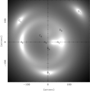
Figure 18: Lensing image of four sources A, B, C & D located at the same redshift $z=3.8$. ${\rm A_{0}}$, ${\rm B_{0}}$, ${\rm C_{0}}$, ${\rm D_{0}}$ denotes the positions of the sources as observed in the absence of the cluster. ${\rm A_{1}}$, ${\rm A_{2}}$, ${\rm B_{1}}$, ${\rm C_{1}}$ and ${\rm D_{1}}$ are the corresponding lensed images.

On the source plane, the caustic defined by the first case is a critical point whereas the caustic defined by the second is a ring. These caustics are called the point caustic and outer caustic, respectively. A point source at the point caustic produces a ring of radius $\theta_{e}$ on the image plane (i.e. the Einstein ring); a point source on the outer caustic is observed as a double source with one radially elongated and reversed image at $\theta=\theta_{c}$ and a second tangentially elongated image at $\theta>\theta_{e}$. In general a point source located outside the outer caustic produces a unique lensed image while a triple image is obtained if the source lies within the outer caustic (Blandford & Narayan, 1992).

As an illustration of the lensing properties of our cluster, in Fig. 18 we show a lensed image of four extended sources A, B, C & D. Each source is located at the same redshift $z=3.8$ and is assumed to be circularly symmetric. Sources B, C, D lie outside the outer caustic whereas A is positioned on the caustic itself. We note the double image (almost triple on the figure) produced by A and its tangential/radial characteristics. The positions of the sources as observed without the lens are indicated so that the lensing effect of the cluster can be fully appreciated.

It is also interesting to note the effect of the lens on a background of sources at a given redshift with a projected number density (in the absence of the lens) of $N_{0}(\theta)$. In the presence of the lens the observed number density becomes $N(\theta)=N_{0}(\theta)/\mu$, and from Fig. 17 we see that $N(\theta)<N_{0}(\theta)$ for $\theta\la 1$ degree.

5.2 Microwave decrement

Figure 19: Einstein ring radius contours over a range of $\rho_{\rm max}$ and $R_{c}$ values for, from top to bottom, $\theta_{e}=150^{\prime\prime}$, $\theta_{e}=100^{\prime\prime}$ and $\theta_{e}=50^{\prime\prime}$. The solid lines denotes the contours computed assuming a simple static lens with an King density profile. The points are exact calculations for an evolving lens (squares for $\theta_{e}=150^{\prime\prime}$, circles for $\theta_{e}=100^{\prime\prime}$ and triangles for $\theta_{e}=50^{\prime\prime}$).

Table 4: Properties of clusters in Fig. 19. $\theta_{e}$ denotes the Einstein ring radius; $T_{e}$ is the electron temperature in the cluster; $\Delta T_{\rm SZ}$ is the Sunyaev-Zel’dovich decrement and $\Delta T_{\rm RS}$ is the Rees-Sciama decrement.

Cluster	$\theta_{e}$	$T_{e}~{}{\rm(K)}$	$\Delta T_{\rm SZ}$ (${\rm\mu K}$)	$\Delta T_{\rm RS}$ (${\rm\mu K}$)
A	$150^{\prime\prime}$	$2.12\times 10^{7}$	523	306
B	$150^{\prime\prime}$	$1.54\times 10^{7}$	466	283
C	$150^{\prime\prime}$	$1.36\times 10^{7}$	459	274
D	$100^{\prime\prime}$	$2.27\times 10^{7}$	491	201
E	$100^{\prime\prime}$	$1.95\times 10^{7}$	464	185
F	$100^{\prime\prime}$	$1.78\times 10^{7}$	458	178
G	$100^{\prime\prime}$	$1.63\times 10^{7}$	459	172
H	$100^{\prime\prime}$	$1.56\times 10^{7}$	463	169
I	$50^{\prime\prime}$	$2.64\times 10^{7}$	464	117
J	$50^{\prime\prime}$	$2.26\times 10^{7}$	466	87
K	$50^{\prime\prime}$	$2.12\times 10^{7}$	490	79

In this section we investigate the contribution of the Rees-Sciama effect to the total temperature decrement reported towards the quasar pair PC1643+4631 A&B and discuss the possibility that the quasars are gravitationally lensed images of the same object (Dabrowski et al. 1997; Dabrowski 1997).

In order to obtain any quantitative results we need to constrain our model parameters. We suppose that both quasars have a redshift $z=3.8$ and that the cluster lies at $z=1$. As for Section 5.1, we assume that $\Omega(t)=1$, $H(t_{0})=50~{}{\rm km~{}s^{-1}~{}Mpc^{-1}}$ and that the total gravitational mass over baryonic mass ratio is $10$. The initial perturbation is for $m=3$. Two parameters remains to be fixed: $\rho_{\rm max}$, the maximum baryonic density encountered by an observed photon and the characteristic core radius $R_{c}$ of the cluster at the time the photon reaches the point of maximum density. To fix these parameters, we have two observational constraints: the quasar pair separation of 198 arcsec and the total flux observed by the Ryle Telescope of $-380~{}{\rm\mu Jy}$ (Jones et al. 1997).

We first consider the lensing separation. Naturally, our spherically-symmetric model cannot account for multiple images that do not lie on the same radial line from the centre of the cluster, as in the case of PC1643+4631 A&B. We note here that a more suitable elliptical setup might present a longer projected line of sight and so enhance the CMB decrement effect. For the purpose of this paper, we consider the Einstein diameter $2\times\theta_{e}$ to be characteristic of the lensing power of the cluster and compare this with the separation of the quasar images. For each pair of values $\rho_{\rm max}$ and $R_{c}$, which describe the cluster central density and core radius, we obtain a value for the Einstein ring radius $\theta_{e}$. The solid lines in Fig. 19 are contours in $(\rho_{\rm max},R_{c})$-space corresponding to Einstein ring radii of $\theta_{e}=50$, 100 and 150 arcsec respectively, calculated without using our model but assuming a static lens with a density distribution described by a King profile (see equation 7). In this case the Einstein ring radius may be found simply by solving numerically the standard equation

$$\theta_{e}=\sqrt{\frac{4GM(\theta_{e})}{c^{2}}\frac{D_{\theta}^{oc}}{D_{\theta}^{os}D_{\theta}^{cs}}},$$ (11)

where $M(\theta_{e})$ is the projected mass included within the radius $\theta_{e}$, $D_{\theta}^{oc}$ denotes the angular-size distance from the observer to the cluster, $D_{\theta}^{os}$ the angular-size distance from the observer to the source and $D_{\theta}^{cs}$ the angular-size distance from the cluster to the source (see Fig. 15). These distances were computed using the formulae given by Blandford & Narayan (1992).

In Fig. 19, we also plot 11 selected cluster setups that have been computed using exact calculations from our evolving spherical cluster model. Since these points represent evolving lenses, and the corresponding clusters do not have exact King density profiles, we see that these points lie slightly away from the contours. The points plotted have been chosen so that A, B, C denote lenses for which $\theta_{e}=150^{\prime\prime}$; D, E, F, G, H have $\theta_{e}=100^{\prime\prime}$ and I, J, K have $\theta_{e}=50^{\prime\prime}$.

Secondly, we consider the total flux observed by the Ryle telescope between the pair of quasars. Table 4 shows the electron temperatures $T_{e}$ required in order that the clusters in Fig. 19 each produce a total observed SZ flux of $-380~{}{\rm\mu Jy}$. Also listed in the table are the corresponding SZ and Rees-Sciama temperature decrements for each cluster. We note that the ratio of the Rees-Sciama effect as compared to the SZ effect varies from $0.61$ for cluster B to $0.16$ for cluster K. Thus in most cases the Rees-Sciama effect is not negligible and might contribute significantly to the total observed CMB decrement. As pointed out in the Introduction, however, we note that these values are to be taken as upper limits.

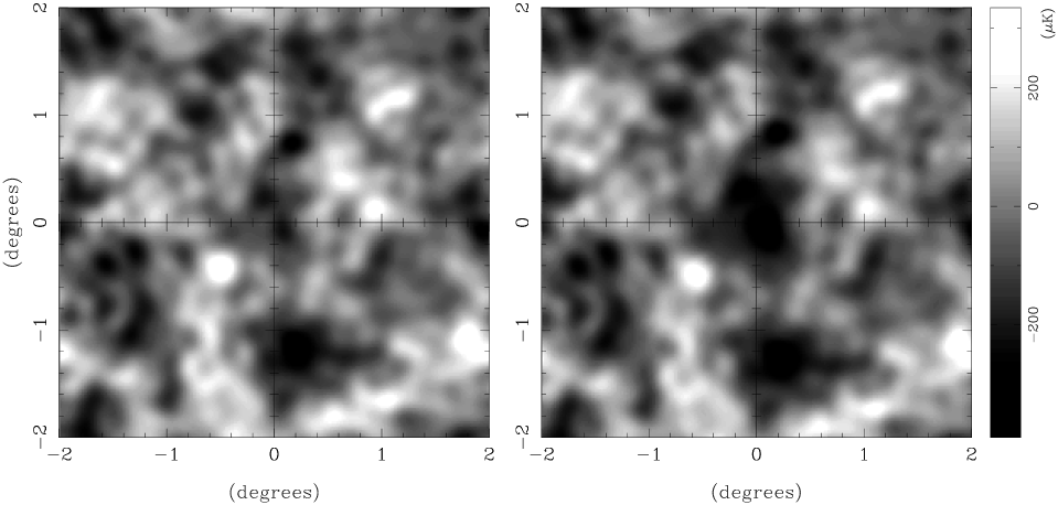
Figure 20: Left: a realisation of CMB fluctuations in a standard inflationary CDM model. Right: the same realisation but with a rich cluster at its centre, producing a Rees-Sciama temperature decrement and gravitational lensing effects.

We take cluster F as a typical example of a cluster which may explain the observations of Jones et al. (1997). The total mass contained within spheres of various radii for cluster F are: $7.8\times 10^{15}~{}{\rm M_{\odot}}$ within 2 Mpc; $1.9\times 10^{16}~{}{\rm M_{\odot}}$ within 4 Mpc; and $4.6\times 10^{16}~{}{\rm M_{\odot}}$ within 8 Mpc. The ratio of the central density to the density of the external Universe at the time the photon passed through the cluster is $\delta=4440$ and the turnaround radius $R_{t}=25.3~{}{\rm Mpc}$.

We may also consider the possible time delay between the light paths for the two quasar images PC1643+4631 A&B. A reasonable approximation may be obtained in our model by considering a source located directly behind the cluster at $z=3.8$ and calculating the time delay between a photon from the source travelling straight through the centre of the cluster and one which follows a lensed path, appearing at the Einstein ring radius $\theta_{e}$. We note that our model takes full account of all the relativistic effects caused by the motions of the source and observer in the Hubble flow and the gravitational effects of the collapsing cluster. We find that the proper time delay in the frame of the source is $\approx 150$ years. This is rather a brief period for the quasar to evolve sufficiently to explain the small redshift difference of the two quasar images.

Finally, we note that observations of the PC1643+4631 field are still in progress. For example, Haynes et al. (1998) carried out deep optical imaging with the William Herschel Telescope and show that the excess of faint blue galaxies in the field might be consistent with a cluster lying at $z\sim 2$. Furthermore, very recent ROSAT observations may suggest that any intervening cluster producing the temperature decrement towards the quasar pair PC1643+4631 A&B should in fact have a redshift $z>3$ (Kneissl 1997; Kneissl, Sunyaev and White 1998). We have therefore repeated our analysis for a cluster lying at a redshift greater than 1 and chosen the (maybe conservative) value of $z=2$. In this case we consider a cluster with a baryonic number density of $10^{4}~{}{\rm m^{-3}}$ and a core radius $R_{c}=0.74~{}{\rm Mpc}$; this ensures an Einstein ring radius of 100 arcsec. The total mass contained within a sphere of 2 Mpc is $1.74\times 10^{16}~{}{\rm M_{\odot}}$, the density ratio $\delta=1313$ and the turnaround radius $R_{t}=22~{}{\rm Mpc}$. In order to retrieve the observed SZ flux of $-380~{}{\rm\mu Jy}$, we require the electron gas temperature of the cluster to be $1.3\times 10^{7}~{}{\rm K}$. This gives an SZ temperature decrement of $547~{}{\rm\mu K}$, while the upper limit of the Rees-Sciama temperature decrement is in this case $\approx 600~{}{\rm\mu K}$ (i.e. it is of the same order as the thermal SZ effect). For such a cluster, we find that the lensing time delay, as described in the previous paragraph, is approximately 230 years in the frame of the emitting source placed at a redshift $z=3.8$.

6 Gravitational lensing of primordial CMB anisotropies

We discussed in the previous section a possible unified model for the formation of a high-redshift cluster with the properties required to produce a microwave decrement and gravitational lensing effects consistent with the observations towards the quasar pair PC1643+4631 A&B. It is also of some interest, however, to investigate the effects of such a cluster on primordial CMB fluctuations.

In this Section, we therefore consider the non-linear gravitational effects on a typical spectrum of primordial fluctuations of the massive cluster F, discussed in the last section, at a redshift $z=1$. These effects include both the gravitational lensing and shift in energy of CMB photons passing through the cluster. We do not, however, include any SZ effect that the cluster may produce.

The effect on primordial fluctuations is investigated by propagating through the evolving cluster a population of CMB photons due to a typical primordial CMB field. It will be seen from Fig. 16 that the reduced deflection angle produced by this cluster falls to zero only at large angles of about 3 degrees. We therefore take as our typical primordial CMB field a $4\times 4$-degree realisation of CMB fluctuations in a standard inflationary Universe dominated by cold dark matter.

Fig. 20 shows that effect of the cluster lying at the centre of the field of primordial CMB fluctuations. We see that the cluster produces a pronounced Rees-Sciama decrement as well as causing a slight radial stretching of the CMB fluctuations which extends as far as the edge of the field.

6.1 Massive cluster abundances

We may also consider the effect of a population of such clusters on the CMB power spectrum. As seen in previous work (e.g. Eke, Cole & Frenk 1996) standard models using the Press-Schechter formalism in a $\Omega_{0}=1$ Universe predict no structure of mass $\sim 10^{15}M_{\odot}$ at redshift greater than $z\sim 0.8$. However counts of clusters are sensitive to $\Omega_{0}$ so that open cosmological models with $\Omega_{0}\sim 0.3$ allow the presence of massive clusters at $z>1$. Eke et al. (1996) extended the Press-Schechter formalism to flat cosmological models with a cosmological constant $\Lambda$ so that $\Omega_{\Lambda}+\Omega_{0}=1$, where $\Omega_{\Lambda}=\Lambda/(3H_{0}^{2})$. For a given value of $\Omega_{0}$, the redshift distribution of massive clusters is similar in both open and flat cosmological models. We assume here $\Omega_{\Lambda}+\Omega_{0}=1$ and a cold dark matter model. We have used the formalism and normalisation described in Eke et al. (1996). The number density of clusters with mass between $M$ and $M+dM$ at a given redshift $z$ is given by $n(z,M)dM$ with

$$n(z,M)=\left(\frac{2}{\pi}\right)^{\frac{1}{2}}\left(\frac{M}{M_{8}}\right)^{\alpha}\frac{\bar{\rho_{0}}\alpha\delta_{c}(z)}{\sigma_{8}M^{2}}\exp^{-\frac{1}{2}\left[\frac{\delta_{c}(z)}{\sigma_{8}}\left(\frac{M}{M_{8}}\right)^{\alpha}\right]^{2}}$$ (12)

where $M_{8}$ is the mass contained in spheres of radius $8h_{0}^{-1}$ Mpc; $\sigma_{8}=0.52\Omega_{0}^{-0.52+0.13\Omega_{0}}$ is the rms linear fluctuation amplitude within $8h_{0}^{-1}$ Mpc spheres;

$$\bar{\rho_{0}}=\frac{3H_{0}^{2}}{8\pi{\rm G}}\left(1-\Omega_{\Lambda}\right)$$ (13)

is the present mean density of the Universe; $\alpha=(0.68+0.4\Gamma)/3$ (see White, Efstathiou and Frenk 1993) for $\Gamma=\Omega_{0}h_{0}=0.25$; and $\delta_{c}(z)$ is the density threshold for collapse as derived in Eke et al. (1996) in the case $\Omega_{\Lambda}+\Omega_{0}=1$. The number of clusters of mass from $M$ to $M+dM$ within a spherical shell extending from $z$ to $z+dz$ is given by $n(z,M)dMdV$ with $dV=4\pi D^{2}dr$ where $D$ is the effective distance and $dr$ is the comoving radial coordinate element equal to $-(1+z)cdt$. Therefore

$$dV=-4\pi cD^{2}(1+z)\frac{\partial{t}}{\partial{z}}dz$$ (14)

where $\partial{t}/\partial{z}$ and $D$ are derived from Fukugita et al. (1992) for the $\Omega_{\Lambda}+\Omega_{0}=1$ case:

$$\frac{\partial{t}}{\partial{z}}=-\left[H_{0}(1+z)\sqrt{3\Omega_{0}z(1+z)+1+\Omega_{0}z^{3}}\right]^{-1},$$ (15)

and

$$D=\frac{c}{H_{0}}\int_{0}^{z}{\frac{dz}{\sqrt{\Omega_{0}(1+z)^{3}+(1-\Omega_{0})}}}$$ (16)

We use the above formulae and find the distributions given in Figs. 21 & 22.

Figure 21: The number of clusters with mass larger than $10^{15}h_{0}^{-1}M_{\odot}$ per unit redshift in the whole sky, as predicted by the Press-Schechter formalism. We assume $\Omega_{0}=0.3$, $\Omega_{0}+\Omega_{\Lambda}=1$ and the normalisation of Eke et al. (1996)

Figure 22: The number of clusters with mass larger than $10^{15}h_{0}^{-1}M_{\odot}$ at a distance further than the given redshift $z$ in the whole sky, as predicted by the Press-Schechter formalism. The lower, middle and upper curves are for $\Omega_{0}=0.3$, $\Omega_{0}=0.23$ and $\Omega_{0}=0.17$ respectively and $\Omega_{0}+\Omega_{\Lambda}=1$ is assumed in each cases. The normalisation is that of Eke et al. (1996)

Fig. 21 shows that for $\Omega_{0}=0.3$ only very few clusters more massive than $10^{15}M_{\odot}$ are expected at redshift larger than 1. Fig. 22 gives the estimated number of $10^{15}M_{\odot}$ clusters in the whole sky as a function of redshift, for various value of $\Omega_{0}$. For $\Omega_{0}=0.3$, $0.23$ and $0.17$ there are, in the whole sky, $\sim 4$, $40$ and $400$ clusters respectively at $z>1$ and more massive than $10^{15}M_{\odot}$. We note that the presence of massive objects as distant as PC1643 may suggest that results using Press-Schechter formalism in a standard cosmology underestimate massive cluster counts at high redshift. This is the reason why, in addition to the realistic assumption $\Omega_{0}=0.3$ (e.g. Webster et al. 1998), we are considering here $\Omega_{0}=0.23$ and $\Omega_{0}=0.17$ which give abundances respectively $10$ times and $100$ times higher than those expected for $\Omega_{0}=0.3$.

6.2 Effect on the CMB power spectrum

The presence of $4$ clusters in the whole sky corresponds roughly to one cluster observed in every $100\times 100$-degree field on the sky, while $40$ clusters correspond to one cluster every $31\times 31$-degree field and $400$ to one cluster every $10\times 10$-degree field. We performed, for these 3 cases, Monte-Carlo simulations of the gravitational effect of the clusters on realisations of primordial CMB fluctuations, and measured the corresponding power spectra. Averaging these measured spectra, we obtain an estimate of the ensemble average power spectrum of CMB fluctuations in the presence of each proposed cluster population. The results are shown in Fig. 23, where they are compared to the ensemble average power spectrum predicted in the absence of clusters. We note that our cluster formation model has been developed for $\Omega_{0}=1$ and $\Omega_{\Lambda}=0$, while abundances have been estimated for $\Omega_{0}+\Omega_{\Lambda}=1$ (see Section 6.1). We will investigate the effect of on our model of $\Omega_{0}\neq 1$ and $\Omega_{\Lambda}\neq 0$ in future work.

Figure 23: Effect on the CMB power spectrum of a population of rich cluster of galaxies. Upper panel: the solid curve is the unperturbed power spectrum while the dashed curve represents the ‘lensed’ spectrum if $400$ clusters are present in the whole sky. Lower panel: the curves are the difference between the predicted unperturbed power spectrum and the ‘lensed’ spectrum for three different cluster abundances corresponding to $400$ (dashed curve), $40$ (dashed-dot curve) and $4$ (dotted curve) clusters in the whole sky.

It is clear that the effect is negligible if only $4$ clusters are present in the sky. However, for abundances where $40$ or $400$ clusters are present in the whole sky, which correspond to $\Omega_{0}\sim 0.2$, the effect is more pronounced and results in smoothing out of the Doppler peaks in the inflationary power spectrum. Therefore, the possibility of such an effect should be taken into account when determining cosmological parameters from future CMB observations. These results are in reasonable agreement with the weak lensing analytical calculations of Seljak (1996) or Martínez-González & Sanz (1997).

7 Conclusions

We apply a new model for the formation of nonlinear cosmic structures (Paper I) to the collapse of spherical clusters of galaxies. The external, expanding Universe and the collapsing cluster are governed by the same pressureless fluid equations. These equations are exact general-relativistic solutions of Einstein equations and no approximations have been made. The initial conditions for the fluid at an early epoch ($z=1000$) are very simple: we impose a finite perturbation on the fluid velocity field that is determined by only three parameters and the corresponding density perturbation is inferred assuming that the perturbation arose from primordial fluctuations.

In Section 3 we studied the formation of a cluster at a redshift $z=0.08$ and found that density profile and mass distribution of the resulting cluster are realistic. We also computed several characteristic quantities for the cluster, such as the total mass contained within spheres of various radii; the ratio of the central density to that of the external Universe ($\delta$); and the turnaround radius ($R_{t}$). Comparing our results with previous authors (e.g. Panek 1992; Quillis 1995), we find reasonable agreement.

Since photon paths are also easily calculated in our model, in Section 4 we studied the gravitational effect of the collapsing cluster on CMB photons (i.e. the Rees-Sciama effect). For a photon traversing the centre of the cluster, we found a central temperature decrement $\Delta T/T\sim-1\times 10^{-5}$ which is in reasonable agreement with previous estimates.

Since our model is most relevant to clusters with large infall velocities, in Section 5 we apply it to clusters with a redshift of $z\geq 1$. Indeed, such high-redshift clusters are more likely to be in a state of free-fall collapse than the low-redshift clusters considered in Sections 3 and 4. In particular, we use our model in an attempt to describe the microwave decrement reported towards the quasar pair PC1643+4631 A&B (Jones et al. 1997). Since the quasar pair is possibly lensed (Saunders et al. 1997), we investigated in Section 5.1 the lensing properties of a cluster which may explain the observations. We find that for such a cluster lensing occurs out to large projected angles $\theta$ from its centre, with an appreciable effect still visible at $\theta=2$ or 3 degrees (see Fig. 16).

In Section 5.2 we consider the relative contributions of the Rees-Sciama and thermal SZ effects to the microwave decrement observed towards PC1643+4631 A&B, and show that the Rees-Sciama effect might contribute significantly for clusters that can simultaneously produce the required lensing properties discussed by Saunders et al. (1997). At $z=1$, such a cluster would have a typical central number density of $10^{4}~{}{\rm m^{-3}}$ and a core radius of $R_{c}=0.45~{}{\rm Mpc}$ (52 arcsec). The total mass contained within a sphere of radius 2 Mpc is then $7.8\times 10^{15}~{}{\rm M_{\odot}}$. We also find, however, that in this scenario the time delay between the light paths for the two quasars images PC1643+4631 A&B is approximately 150 years, as measured in the frame of the (lensed) quasar. This period might be rather short to explain the slight redshift difference between the two quasar images. Following very recent ROSAT observations of PC1643+4631 A&B by Kneissl (1997), which suggest that any intervening cluster should be at an even greater redshift, we also repeat our calculations for a similar cluster at a redshift $z=2$. We find a typical core radius of $R_{c}=0.74~{}{\rm Mpc}$ (90 arcsec) for a central number density of $10^{4}~{}{\rm m^{-3}}$. The total mass contained within a sphere of radius 2 Mpc is $1.74\times 10^{16}~{}{\rm M_{\odot}}$.

Finally, in Section 6, we consider the effect on primordial microwave background fluctuations of a population of massive clusters, such as that described in Section 5. We find that in the case of cluster abundances corresponding to a $\Omega_{0}\sim 0.2$ and $\Omega_{0}+\Omega_{\Lambda}=1$ cosmological model, the Doppler peaks of the CMB power spectrum are slightly smoothed out by the lensing effects (see Fig. 23), confirming weak lensing the results in Seljak (1996) and suggesting that this effect should be taken into account when determining cosmological parameters.

References

- [1] Arnau J., Fullana M., Monreal L., Sáez D., 1993, ApJ, 402, 359
- [2] Arnau J., Fullana M., Sáez D., 1994, MNRAS, 268, L17
- [3] Bartlett J.G., Blanchard A., Barbosa D., Oukbir J., 1997, in The Particle Physics and the Early Universe Conference, Cambridge, April 1997∗.
- [4] Blandford R.D., Narayan R., 1992, ARAA, 30, 311
- [5] Chodorowski M., 1991, MNRAS, 251, 248
- [6] Dabrowski Y., 1997, Acta Cosmologica, in press
- [7] Dabrowski Y., Hobson M.P., Lasenby A.N., Doran C., 1997, in The Particle Physics and the Early Universe Conference, Cambridge, April 1997∗.
- [8] Deltorn J.M., Le Fevre O., Crampton D., Dickinson M., 1997, ApJ, 483, L21
- [9] Dyer C.C., 1976, MNRAS, 175, 429
- [10] Eke V.R., Cole S., Frenk C.S., 1996, MNRAS, 282, 263
- [11] Fukugita M., Futamase T., Kasai M., Turner E.L., ApJ, 393, 3
- [12] Fullana M.J., Sáez D., Arnau J.V., 1994, ApJS, 94, 1
- [13] Haynes T., Cotter G., Baker J., Eales S., Jones M., Rawlings S., Saunders R., in preparation.
- [14] Jones C. and Forman W., 1984, ApJ, 276, 38
- [15] Jones M.E. et al., 1997, ApJ, 479, L1
- [16] Kaiser N., 1982, MNRAS, 198, 1033
- [17] Kneissl R., Sunyaev R.A. and White S.D.M, 1998, MNRAS, 297, L29
- [18] Kneissl R., 1997, in The Particle Physics and the Early Universe Conference, Cambridge, April 1997∗.
- [19] Kravtsov A.V., Klypin A.A., Bullock J.S., Primack J.R., 1998, ApJ, 502, 48
- [20] Lasenby A.N., Doran C., Gull S.F., 1998, Phil. Tran. R. Soc. Lond. A, 356, 487
- [21] Lasenby A.N., Doran C., Hobson M.P., Dabrowski Y., Challinor A.D., 1998, Microwave background anisotropies and nonlinear structures I. Improved theoretical models, submitted to MNRAS
- [22] Luppino G.A. and Kaiser N., 1997, ApJ, 475, 20
- [23] Martínez-González E., Sanz J.L., 1990, MNRAS, 247, 473
- [24] Martínez-González E., Sanz J.L., 1997, ApJ, 484, 1
- [25] Martínez-González E., Sanz J.L., Silk J., 1990, ApJ, 335, L5
- [26] Navarro J., Frenk C., White S., 1996, ApJ, 462, 563
- [27] Nottale L., 1982, A&A, 110, 9
- [28] Nottale L., 1984, MNRAS, 206, 713
- [29] Panek M., 1992, ApJ, 388, 225
- [30] Peebles P.J.E., in Principles of Physical,Cosmology, Princeton University Press, 1993, p 587
- [31] Quilis V., Ibáñez J.M., Sáez D., 1995, MNRAS, 277, 445
- [32] Quilis V., Sáez D., 1998, MNRAS, 293, 306
- [33] Rees M.J., Sciama D.W., 1968, Nat, 217, 511
- [34] Refsdal S., 1964, MNRAS, 128, 295
- [35] Richards E.A., Fomalont E.B., Kellermann K.I., Partridge R.B., Windhorst R.A., 1997, AJ, 113, 1475
- [36] Rood H.J, Page T.L., Kintner E.C., King I.R., 1972, ApJ, 175, 627
- [37] Sáez D., Arnau J.V., Fullana M.J., 1993, MNRAS, 263, 681
- [38] Saunders R. et al., 1997, ApJ, 479, L5
- [39] Sarazin G.L., in X-ray emissions from clusters of galaxies, Cambridge University Press, 1988, p 168
- [40] Seljak U., 1996, ApJ, 463, 1
- [41] Webster M., Hobson M.P., Lasenby A.N., Lahav O., Rocha G., 1998, submitted to ApJL
- [42] White S.D.M., Efstathiou G., Frenk C.S., 1993, MNRAS, 262, 1023
- [43] Zhao H., 1996, MNRAS, 278, 488 00footnotetext: http://www.mrao.cam.ac.uk/ppeuc/proceedings/cmb_prog.html