EUVE Spectroscopy of Polars
Abstract
An admittedly pedantic but hopefully useful and informative analysis is presented of the EUVE 70–180 Å spectra of nine polars. These spectra are fit with three different models—a blackbody, a pure-H stellar atmosphere, and a solar abundance stellar atmosphere—to reveal the presence of spectral features such as absorption lines and edges, and to investigate the sensitivity of the derived (, , solid angle) and inferred (fractional emitting area, bolometric luminosity) parameters to the model assumptions. Among the models tested, the blackbody model best describes the observed spectra, although the untested irradiated solar abundance stellar atmosphere model is likely a better overall description of the EUV/soft X-ray spectra of polars.
1998, Proceedings of the Annapolis Workshop on Magnetic Cata-
clysmic Variables, ed. C. Hellier & K. Mukai (San Francisco: ASP)
Lawrence Livermore National Laboratory, CA, U.S.A. and
Department of Physics, Keele University, Staffordshire, U.K.
1. Introduction
When all is said and done, the accreting material that causes all the fireworks in a magnetic CV finds itself channeled onto a small spot on the white dwarf surface in the vicinity of the magnetic pole(s). The extremes of this accretion region are masked from us by the units we typically employ to describe it: translated into more familiar units, a shock temperature of 10 keV equals 100 million degrees; an accretion rate of equals 7 billion tons per second; an accretion luminosity of is the equivalent energy release of megaton bombs per second. All this energy is released above and into an area of times the surface area of the white dwarf—an area of , which is about the size of California.
The energy input into the accretion region is supplied by radiative heating from above by the keV thermal plasma below the accretion shock and by mechanical heating by blobs of material which punch through the shock and penetrate into the stellar surface before thermalizing their kinetic energy. The equilibrium photospheric temperature of the region is then determined by the balance of radiative and mechanical heating and radiative cooling, with the latter dependent upon such factors as the surface area of the accretion region and the sources of opacity (i.e., metallicity) and the ionization state of the photosphere. For a luminosity of and a fractional emitting area of , the blackbody temperature of the region is eV.
Unfortunately, it is observationally challenging to accurately determine the spectral parameters of a eV blackbody: its peak (in ) lies at Å or keV where the energy resolution of ionization-type detectors is poor and photoelectric absorption is severe. Worse, dispersive instruments do not give consistent results for AM Her, by far the brightest polar: the best-fit parameters of a blackbody fit to the Einstein OGS spectrum of AM Her are eV and (Heise et al. 1984), the parameters for the EXOSAT TGS spectrum are eV and (Paerels, Heise, & van Teeseling 1994), and those for the EUVE SW spectrum are eV and (Mauche, Paerels, & Raymond 1995). The inability to derive consistent results from grating observations of the brightest polar should warn us not to take too seriously the parameters—both direct (, , solid angle) and inferred (fractional emitting area, bolometric luminosity)—derived from such simple model fitting. A much better approach is to look for trends in the spectral parameters of a sample of systems analyzed in a consistent manner, and to investigate the sensitivity of the derived parameters to the model assumptions. Such is just the purpose of this presentation.
2. EUVE Spectra
Until the launch of AXAF later this year, there is a single satellite capable of dispersive spectroscopy of the soft spectral component of magnetic CVs: the Extreme Ultraviolet Explorer (EUVE; Bowyer & Malina 1991; Bowyer et al. 1994). The salient features of EUVE’s SW spectrometer are its 70–180 Å bandpass, its 0.5 Å spectral resolution, and its relatively small effective area ( at 100 Å). The last attribute means that bright targets and long integrations are required to obtain useful EUV spectra, and integrations of 50–100 kiloseconds are consequently typical. Such long integrations assure that all binary orbital phases are sampled, but the low count rates typically do not allow studies of the orbital phase dependence of the spectra. While the width of the SW bandpass is nominally a factor of 2.6, it is typically effectively much narrower because of photoelectric absorption of EUV photons by material within the binary (e.g., the accretion stream and column) and the interstellar medium between the source and Earth; unit optical depth is reached for a column density of , , , , and at , 250, 150, 100, and 65 Å, respectively.
At the present time (1998 August), there are 17 magnetic CVs with EUVE spectra in the public archive (for a general discussion of these and other EUVE spectra, see Craig et al. 1997). Only 2 of these 17 systems are intermediate polars (EX Hya and PQ Gem), and since papers have been published on both of these systems (Hurwitz et al. 1997 and Howell et al. 1997, respectively), their spectra will not be discussed here. Of the 15 polars, only 11 have “useful” spectra, and details of the relevant observations of these 11 systems are collected in Table 1. The columns in that table are as follows. The second column is the UT date of the start of the observation. The third column is the Primbsch/deadtime corrected exposure time for the SW image. The fourth column indicates whether the spectrum was dithered (delightfully, to “dither,” is to “shiver” or “tremble”) on the face of the detector to eliminate the detector fixed-pattern noise; well-exposed non-dithered spectra have non-statistical errors in the derived flux densities which artificially increase the of fits to the data. The fifth column reports the maximum signal-to-noise ratio of the data in 0.54 Å bins. Finally, for completeness, the sixth column supplies a reference to a previous work with some discussion of the EUVE spectrum of each source. For all of the sources except AM Her, the given reference deals with the same spectrum as that discussed herein; the reference for AM Her is for the paper on the original (1993 September) undithered observation of that source. Like AM Her, QS Tel has been observed repeatedly by EUVE, and for both of these sources we have extracted from the archive the longest single exposure.
| TABLE 1 | |||||
| Journal of Observations | |||||
| Start Date | Exposure | ||||
| Source | (UT m/d/y h:m) | (ksec) | Dithered? | S/N | Ref.a |
| AM Her | 03/08/95 12:19 | 123.3 | Yes | 46 | 1 |
| AN UMa | 02/27/93 22:15 | 41.1 | No | 2.5 | 2 |
| AR UMa | 12/14/96 09:25 | 93.7 | Yes | 22 | |
| BL Hyi | 10/30/95 07:37 | 39.8 | No | 8 | 3 |
| EF Eri | 09/05/93 13:42 | 95.7 | No | 7 | 4 |
| QS Tel | 10/06/93 07:51 | 69.5 | No | 13 | 5 |
| RE J1149284 | 12/26/94 06:06 | 114.3 | Yes | 2.5 | |
| RE J1844741 | 08/17/94 13:58 | 134.6 | No | 8 | |
| UZ For | 01/15/95 20:38 | 78.5 | Yes | 7 | 2 |
| VV Pup | 02/07/93 21:24 | 43.6 | No | 5 | 6 |
| V834 Cen | 05/28/93 03:06 | 41.3 | No | 8 | 2 |
aReferences: 1: Paerels et al. 1996b; 2: Warren 1998; 3: Szkody et al. 1997; 4: Paerels et al. 1996a; 5: Rosen et al. 1996; 6: Vennes et al. 1995.
For the record, the reduction of the archival data was accomplished as follows. The SW image was extracted from the FITS data file, while the effective exposure time and wavelength parameters were extracted from the FITS header. The centerline of the spectrum was determined by forming a projection of the SW image onto the imaging axis. The source region was taken to be this centerline lines (e.g., lines 137–157), while the background region was taken to be 84 lines above and below the source region beyond a gap of 10 lines (e.g., lines 44–127 and 167–250). The source and background spectra are the sum of the counts in these regions within each wavelength bin, and the net spectra and errors were calculated accordingly after binning in wavelength by a factor of 8 (from Å to 0.539 Å). This wavelength binning matches the spectral resolution of the SW detector, hence any intrinsically narrow absorption or emission features will appear predominantly in one wavelength bin. It is at this binning that the signal-to-noise ratio values shown in Table 1 were derived. The two systems in that table with peak signal-to-noise ratios below 3 (AN UMa and RE 1149) were not considered further.
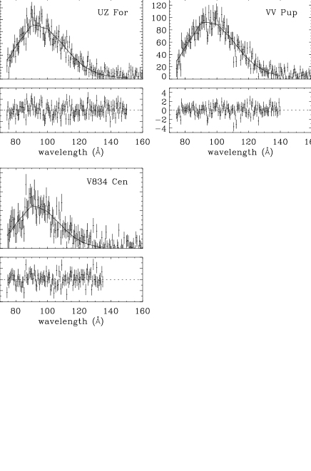
![[Uncaptioned image]](/html/astro-ph/9810116/assets/x1.png)
The resulting spectra (in counts per 0.54 Å bins versus wavelength) of the 9 surviving sources are shown in Figure 1. The shape of these spectra naturally mimic the shape of the effective area curve, which peaks at 100 Å and falls off at both ends of the bandpass. Of the count distributions shown in Figure 1, that of AR UMa is the softest, as it peaks at Å and not only extends all the way down to 180 Å in the SW channel, but even manifests itself on the “left” end of the MW channel (150–350 Å). In contrast, the count distribution of AM Her is among the hardest of the sources shown, as it peaks at Å and falls off rapidly at longer wavelengths. Note, however, that while the long-wavelength ( Å) flux of AM Her is small, it is not zero; indeed, the count distribution rises longward of Å. Given the exponential form of photoelectric absorption, this apparent long-wavelength flux is almost certainly due to “contamination” of the first-order spectrum by higher orders. While the second- and third-order diffraction efficiencies of the EUVE spectrometers were measured in the laboratory prior to launch, it is less clear that they were calibrated in orbit. To minimize the possible uncertainties of the higher-order diffraction efficiencies, we ignore the data longward of some wavelength where higher-order flux may dominate the first-order flux. For AM Her, we take this cutoff to be at 130 Å; for the other sources, it ranges from 135 to 180 Å. The short-wavelength limit of the spectra is fixed at 74 Å; shortward of that wavelength there is a rapid increase in the background.
To allow a quantitative assessment of the spectra shown in Figure 1, these data were fit with three different spectral models—a blackbody, a pure-H stellar atmosphere, and a solar abundance stellar atmosphere—all extinguished at long wavelengths by photoelectric absorption. For the latter, we take the EUV absorption cross sections of Rumph, Bowyer, & Vennes (1994) for H i, He i, and He ii with abundances ratios of 1:0.1:0.01, as is typical for the diffuse interstellar medium. While this choice for the abundance ratios is standard, it is decidedly non-trivial, since the slopes of the absorption cross sections of the various ions differ somewhat in the EUV. For the chosen ratios, the photoelectric opacity in the SW bandpass is dominated by He i, while for much more highly ionized gas (e.g., the accretion stream and column), He ii may dominate. Furthermore, partial covering may allow an excess of EUV photons to escape the binary, but to be detected at Earth, these rogue photons must still make their way through the ISM without getting clobbered.
3. Blackbody Fits and General Comments
The blackbody fits to the EUVE spectra are the simplest to calculate as well as to describe, hence we begin with those. The fits of this model to the EUVE data and the resulting residuals are shown in Figure 1, while the 68, 90, and 99% confidence contours are shown in Figure 2, and the 90% confidence fit parameters (, , solid angle, 70–140 Å flux, bolometric flux, /dof) are listed in Table 2. First consider the best-fit models and residuals shown in Figure 1.
Blackbodies may or may not be an accurate description of the intrinsic EUV spectra of polars, but this model is smooth and hence its residuals reveal the presence of spectral features such as lines and edges. The number of possible discrete transitions in the SW bandpass is huge, but among the abundant elements, possible absorption edges include N v, O v–vi, Ne iv–vi, Mg iii–v, S vi, Ar vi–viii, Ca v–viii, and Fe vi–viii. Because of the high density of the white dwarf photosphere, there are in addition to the ground-state edges (e.g., the O vi edge at 89.8 Å and the Ne vi edge at 78.5 Å), edges from excited states of these ions (e.g., the O vi edge at 98.3 Å and the Ne vi edge at 85.2 Å). O vi edges were identified by Vennes et al. (1995) in the spectrum of VV Pup, Ne vi edges were identified by Paerels et al. (1996b) in the 1993 September spectrum of AM Her, and the Ne vi edge was identified by Rosen et al. (1996) in the spectrum of QS Tel. The edge in the QS Tel spectrum is just visible in Figure 1 as a discontinuous jump at 85 Å in the residuals for this source, but the putative edges of AM Her and VV Pup are less obvious. Perhaps the most obvious jump in the residuals is manifest by V834 Cen at 85 Å, again implicating Ne vi. The problem with detecting edges this way is that there are medium- and low-frequency residuals present at some level in almost all of the spectra, even though the reduced of the fits listed in Table 2 indicate that for most of the sources the fits are acceptable.
It is more straightforward to detect discrete features in these spectra, since the spectral binning is set to match the resolution of the SW instrument and because such features are apparent almost regardless of the adopted spectral model. With the exception of AM Her, there are no sources with discrete residuals greater than (i.e., emission lines), while nearly all of the sources show discrete residuals less than (i.e., absorption lines). The features with the highest significance in one spectral bin are found in the residuals of AM Her (76.1, 98.2 Å), AR UMa (116.5 Å), and QS Tel (98.2, 116.5 Å). These are the very sources with the highest signal-to-noise ratio spectra (), suggesting the possibility that similar features could be detected in all of the sources if the integrations were long enough. The 98 Å feature is identified as Ne viii - and was observed first by Paerels et al. (1996b) in the 1993 September EUVE spectrum of AM Her, and subsequently by Rosen et al. (1996) in the spectrum of QS Tel; in the new dithered spectrum of AM Her this feature is so strong (and the signal-to-noise ratio so high) that it is readily apparent in the raw data. The 116.5 Å feature was observed first by Rosen et al. in QS Tel and is identified as Ne vii -; we now identify this feature in AR UMa as well. Other reasonably narrow and apparently real absorption features are found in the residuals of AR UMa (108.7 Å), BL Hyi (92.9 Å), EF Eri (96.5 Å), VV Pup (94.1 Å), but their identifications are uncertain.
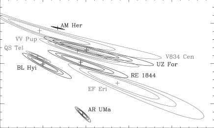
The surface for the blackbody fits to the EUVE data is shown in Figure 2, which shows that within the 90% confidence contours, the blackbody temperature ranges between 13.4 and 20.3 eV (156–236 kK). On the orthogonal axis, the hydrogen column density ranges from a low of for AR UMa to a high of for AM Her. If this value for for AM Her is physical and not simply a parameterization of the data, most of the absorbing column must be ionized and hence within the binary, since the neutral hydrogen column density to this source is (Gänsicke et al. 1998). Table 2 lists the corresponding 90% confidence parameters for these blackbody fits. Note that the reduced of the fits to AM Her, AR UMa, EF Eri, and QS Tel are not acceptable, so the fit parameters should be taken only as indicative. For a given distance to a given source, the tabulated values of the solid angle and bolometric flux can be used to derive such useful quantities as the fractional emitting area and the bolometric luminosity.
4. Pure-H Stellar Atmosphere Fits
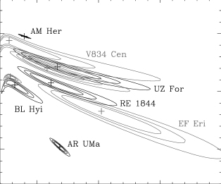
The second model used to fit the EUVE spectra was that of a pure-H, line-blanketed, NLTE, stellar atmosphere calculated with TLUSTY (Hubeny 1988). The surface of the fits of these models to the data is shown in Figure 3. Notice that the relative ordering of these Daliesque contours is very similar to that of the blackbody fits, but that the temperatures are systematically much lower: within the 90% confidence contours, the effective temperature ranges between 2.4 and 7.5 eV (28–87 kK). The hydrogen column densities are higher than before, but typically by only 10–20%. The 90% confidence parameters for these fits are again listed in Table 2. Note that the reduced of these fits are essentially identical to those of the blackbody model, hence at that level the pure-H stellar atmosphere model is just as acceptable a description of the data. However, because the EUV bump in the stellar atmosphere models contains a relatively small fraction of the total luminosity, the biggest change between these models is the solid angle, which is now larger by a factor of –. Indeed, in some cases (e.g., AM Her, QS Tel) the derived solid angle is so large that it completely excludes the stellar atmosphere model: since cm and pc, the solid angle must be less than . In other cases, the implied UV flux density will likely exceed the measured value, but such a constraint typically requires that we have simultaneous EUV and UV measurements, which is seldom the case.
5. Solar Abundance Stellar Atmosphere Fits
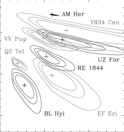
The third and final model used to fit the EUVE spectra was that of a solar abundance stellar atmosphere; specifically, the “un-illuminated” solar abundance model atmospheres of van Teeseling, Heise, & Paerels (1994). The surface of the fits of these models to the data is shown in Figure 4. Table 2 again lists the nominal 90% confidence parameters values for these fits, but note that because the reduced of the fits are unacceptably large the parameters should be understood only to be indicative. With this limitation in mind, we see that the effective temperatures are higher, and the hydrogen column density lower compared to the blackbody and pure-H stellar atmosphere model fits; within the nominal 90% confidence contours, the effective temperature ranges between 22.8 and 27.4 eV (265–318 kK), while the hydrogen column density ranges from a (rather unlikely) low of for AR UMa to a high of for AM Her. This range of parameters is pleasing for two reasons. First, the inferred hydrogen column densities are lower than for the previous models and are more likely to be consistent with the interstellar values. Second, the inferred effective temperatures are now high enough that the accretion region may be capable of producing the soft X-ray fluxes observed by ROSAT (e.g., Beuermann & Burwitz 1995).
![[Uncaptioned image]](/html/astro-ph/9810116/assets/x6.png)
Despite these attractive aspects of the solar abundance stellar atmosphere models, they are in every case an unacceptable description of the data because of their strong O vi absorption edges. The simplest way to remedy this discrepancy is to reduce the O abundance, but there is no other compelling evidence that the material accreted by the white dwarf in polars is significantly underabundant in this element; AM Her for one certainly has a strong O vi emission line in the FUV (Mauche & Raymond 1998). A much more natural and physical explanation of the weakness of the O vi absorption edges is the irradiated stellar atmosphere model (Williams, King, & Booker 1987; van Teeseling, Heise, & Paerels 1994). In that model, irradiation of the white dwarf photosphere by hard X-rays results in a temperature inversion above the photosphere and a flattening of the run of temperature with optical depth within the photosphere. If the temperature profile in the photosphere is flat where the edges and lines form, their strength will be significantly decreased. van Teeseling et al. found that an irradiated stellar atmosphere with an effective temperature of eV ( kK) fit the EXOSAT TGS spectrum of AM Her as well as or better than a blackbody with eV (270 kK). Note, however, that their model requires that more than 96% of the soft X-ray luminosity is due to reprocessing; this leaves little or no room for direct kinetic heating of the photosphere, the favored solution of the famous soft X-ray problem. Furthermore, even the irradiated stellar atmosphere models have strong edges shortward of the EUVE bandpass, so it is not entirely clear that the observed soft X-ray fluxes can be produced.
6. Summary
We have found that, of the blackbody, pure-H stellar atmosphere, and solar abundance stellar atmosphere models, the blackbody model provides the best phenomenological description of the EUVE 70–180 Å spectra of polars. Inadequacies of this model include the weak absorption edges of Ne vi and the absorption lines of Ne vii and Ne viii apparent in the residuals of the sources with the highest signal-to-noise ratio spectra, and the likely inability of these moderately soft blackbodies to produce the observed soft X-ray fluxes. The untested irradiated solar abundance stellar atmosphere model is likely a better overall description of the EUV/soft X-ray spectra of polars, but better models (which include, e.g., absorption lines as well as edges) and better data (e.g., high signal-to-noise ratio phase-resolved AXAF 3–140 Å LETG spectra) are required before significant progress can be made in our understanding of the accretion region of magnetic CVs.
Acknowledgments.
The author is pleased to acknowledge I. Hubeny for his guidance in the proper use of the TLUSTY and SYNSPEC suite of programs, A. van Teeseling for generously providing his grid of solar abundance stellar atmosphere models, B. Gänsicke for his assistance spot checking his and TLUSTY’s pure-H stellar atmosphere models, and the hospitality of the students and staff—particularly A. Evans, R. Jeffries, T. Naylor, and J. Wood—at Keele University where this work was completed. This work was performed under the auspices of the U.S. Department of Energy by Lawrence Livermore National Laboratory under contract No. W-7405-Eng-48.
References
Beuermann, K., & Burwitz, V. 1995, in Cape Workshop on Magnetic Cataclysmic Variables, ed. D. A. H. Buckley & B. Warner (San Francisco: ASP), 99
Bowyer, S., & Malina, R. F. 1991, in Extreme Ultraviolet Astronomy, ed. R. F. Malina & S. Bowyer (New York: Pergamon), 397
Bowyer, S., et al. 1994, ApJS, 93, 569
Craig, N., et al. 1997, ApJS, 113, 131
Gänsicke, B. T., Hoard, D. W., Beuermann, K., Sion, E. M., & Szkody, P. 1998, A&A, in press
Heise, J., et al. 1984, Phys. Scripta, T7, 115
Howell, S. B., et al. 1997, ApJ, 485, 333
Hubeny, I. 1988, Computer Phys. Comm., 52, 103
Hurwitz, M., Sirk, M., Bowyer, S., & Ko, Y.-K. 1997, ApJ, 477, 390
Mauche, C. W., Paerels, F. B. S., & Raymond, J. C. 1995, in Cape Workshop on Magnetic Cataclysmic Variables, ed. D. A. H. Buckley & B. Warner (San Francisco: ASP), 298
Mauche, C. W., & Raymond, J. C. 1998, ApJ, 505, in press
Paerels, F., Heise, J., & van Teeseling, A. 1994, ApJ, 426, 313
Paerels, F., Hur, M. Y., & Mauche, C. W. 1996a, in Astrophysics in the Extreme Ultraviolet, ed. S. Bowyer & R. F. Malina (Dordrecht: Kluwer), 309
Paerels, F., Hur, M. Y., Mauche, C. W., & Heise, J. 1996b, ApJ, 464, 884
Rosen, S. R., et al. 1996, MNRAS, 280, 1121 (note that the units of the y axis of Fig. 6 of this paper should be )
Rumph, T., Bowyer, S., & Vennes, S. 1994, AJ, 107, 2108
Szkody, P., Vennes, S., Sion, E. M., Long, K. S., & Howell, S. B. 1997, ApJ, 487, 916 (note that the units of the y axis in the upper panels of Fig. 2 of this paper should be )
van Teeseling, A., Heise, J., & Paerels, F. 1994, A&A, 281, 119
Vennes, S., Szkody, P., Sion, E. M., & Long, K. S. 1995, ApJ, 445, 921
Warren, J. K. 1998, PhD thesis, Physics Department, UC Berkeley
Williams, G. A., King, A. R., & Booker, J. R. E. 1987, MNRAS, 266, 725