Large-Scale Flows as a Cosmological Probe

Abstract

ABSTRACT. We review the use of peculiar velocities of galaxies as a probe of cosmological models. We put particular emphasis on comparison of the peculiar velocity and density fields, focussing on the discrepancies between various recent analyses. We discuss the limitations of the commonly used linear bias model, which may lie at the heart of some of the current controversies in the field.

ABSTRACT. We review the use of peculiar velocities of galaxies as a probe of cosmological models. We put particular emphasis on comparison of the peculiar velocity and density fields, focussing on the discrepancies between various recent analyses. We discuss the limitations of the commonly used linear bias model, which may lie at the heart of some of the current controversies in the field.

1 Introduction

We believe for a large number of reasons (including those to be outlined in this review) that we live in a universe which is dominated by dark matter. We see galaxies by the light of the stars that shine within them; we can similarly infer the presence of large quantities of hot gas through its X-ray emission, and cold gas through molecular and atomic emission in the millimeter and radio portions of the spectrum. But the baryons that give rise to these emissions comprise at most 10% or so of the mass density of the universe. The study of large-scale structure asks how this dark matter is distributed in space. We cannot observe it directly, but we can infer many of its properties due to its gravitational influence on the matter around it. We observe that the distribution of galaxies is clustered, and make the assumption (which is at least qualitatively justified, as we will see below) that the dark matter distribution is clustered in a similar way. A local overdensity in mass will gravitationally attract the adjacent matter, disturbing the pure Hubble flow; similarly, a local underdensity will gravitationally repel matter. These additional motions, or peculiar velocities, are observable. Therefore, we can use peculiar velocities to get an observational handle on the clustered component of the dark matter. We make these notions concrete as follows. Pure Hubble flow states that redshift is proportional to distance,

$$cz=H_{0}r,$$ (1)

and indeed, if we measure distances in units of $\rm\,km\ s^{-1}$, and never make reference to standard yardsticks calibrated in physical units (e.g., cm or Mpc), the value of $H_{0}$ is identically unity. Peculiar velocities are defined relative to the comoving expanding frame implied by equation (1):

$$cz=r+\hat{\bf r}\cdot\left[{\bf v}({\bf r})-{\bf v}({\bf 0})\right],$$ (2)

where v(r) is the peculiar velocity field, and redshifts are measured relative to the barycenter of the Local Group (as opposed to, e.g., the CMB rest frame). In linear gravitational instability theory one can relate the density fluctuations to the peculiar velocities:

$${\bf v}({\bf r})={\Omega^{0.6}\over 4\,\pi}\int{\rm d}^{3}{\bf r}^{\prime}\,{\delta({\bf r}^{\prime})\,({\bf r}^{\prime}-{\bf r})\over|{\bf r}^{\prime}-{\bf r}|^{3}},$$ (3)

where $\Omega$ is the Cosmological Density Parameter, and the density fluctuation field is defined as:

$$\delta({\bf r})={{\rho({\bf r})-\left\langle\rho\right\rangle}\over{\left\langle\rho\right\rangle}}.$$ (4)

The integral on the right-hand side is just proportional to the gravity vector. As an aside, note that it is manifestly not true that peculiar velocity is proportional to gravity in the highly nonlinear regime: the gravity and velocity vectors of the Earth’s orbit are at right angles to one another! We will also find it useful to express equation (3) in differential form; by taking the divergence of both sides of the equation, one finds:

$$\nabla\cdot{\bf v}({\bf r})=-\Omega^{0.6}\delta({\bf r}).$$ (5)

Note that peculiar velocities, if measured in the linear regime, are a measure of the response of galaxies to the gravitational influence of all matter, and especially the dominant dark matter. Therefore, we can measure the large-scale distribution of dark matter directly from observations of the peculiar velocity field. Moreover, if we have an independent measurement of the large-scale distribution of galaxies from redshift surveys, and a model that relates the galaxy and dark matter distribution, we can use equation (3) or (5) to

• $\bullet$ Test the gravitational instability paradigm from which these equations were derived;

• $\bullet$ Test the assumed model relating the distribution of the dark and luminous matter;

• $\bullet$ Measure the quantity $\Omega$ directly.

2 The Measurement of Peculiar Velocities

Peculiar velocities manifest themselves through their modification to the Hubble Law, equation (2). Therefore, with independent measurements of redshifts and distances of a galaxy, we can measure the radial component of its peculiar velocities. Redshifts are relatively easy to measure; a high-quality galaxy spectrum will show sharp stellar absorption lines, and often strong emission lines that arise from photo-ionized gas in H$\scriptstyle\rm II$ regions or an active nucleus. Distances are quite a bit more difficult; one needs to identify a standard candle (i.e., a distance-independent way to determine the absolute magnitude of the galaxy, or some well-defined component of it), or a standard yardstick (i.e., a characteristic physical size of the galaxy). Comparison with the apparent magnitude or angular size then yields a distance. Reviews of distance indicators used in peculiar velocity work can be found in Jacoby et al. (1992), Strauss & Willick (1995, hereafter SW), and Willick (1998). The Tully-Fisher (1977; TF) relation states that the luminosity and (inclination-corrected) rotation velocity of a spiral galaxy are related by a power law; expressing this in terms of absolute magnitudes, we find:

$$M=A\log\Delta V+B.$$ (6)

Thus, observations of apparent magnitudes $m$ and rotation velocities $\Delta V$ (via the H$\alpha$ line at 6563Å with a long-slit spectrograph placed along the major axis of the galaxy, or the width of the 21 cm line in the radio), yield a distance. The TF relation is not perfect, and shows some appreciable scatter; distances are measured typically to an accuracy of 15-20%. Moreover, the constants $A$ and $B$ depend on the details of sample selection, the band in which the galaxy photometry is done, and so on, and these quantities need to be calibrated carefully for any given TF sample. Since we measure the peculiar velocity as the difference of two rather large quantities (equation 2), the signal-to-noise ratio per galaxy of the peculiar velocity field is typically low, and is a decreasing function of distance. This means that a great deal of care needs to be taken in doing TF work; when data are noisy, there are a number of pernicious systematic effects that can creep into the derived velocity field if one is not careful (cf., the discussion in SW; Teerikorpi 1997). There are a number of other distance indicators that are used in peculiar velocity work:

• $\bullet$ Elliptical galaxies are observed to fall along the so-called fundamental plane (Djorgovski & Davis 1987; Dressler et al. 1987), which relates the luminosity, the surface brightness, and the velocity dispersion or color of galaxies. This yields distances to an accuracy of roughly 20% in distance, comparable to the TF relation.

• $\bullet$ Distances can also be measured to ellipticals using the method of surface brightness fluctuations (Tonry & Schneider 1988). Elliptical galaxies typically have intrinsically smooth surface brightness profiles, unmarred by structural components such as spiral arms or dust lanes. However, their light is generated by a finite number of stars, and the closer the galaxy is to us, the fewer of the red giant stars that dominate the optical light will fall within each seeing element of an image. This number of stars will be subject to Poisson statistics, and therefore the closer the galaxy is to us, the rougher the image will appear. This roughness is therefore a measurement of the distance of the galaxy. This is a method that holds a tremendous amount of promise for peculiar velocity work, as it yields distances to accuracies of 5% for at least some galaxies. Unfortunately, the method is seeing limited, and requires the resolution of the Hubble Space Telescope to reach much beyond 3000 $\rm\,km\ s^{-1}$. Although there now exist substantial data for nearby galaxies using this technique (e.g., Tonry et al. 1997), it has not yet been exploited for studies of the peculiar velocity field in any detail.

• $\bullet$ The most luminous galaxies in clusters have long been recognized to be distinct from the “ordinary” ellipticals that make up the bulk of the galaxy population in ellipticals. Gunn & Oke (1975) and Postman & Lauer (1995) show that the luminosity of Brightest Cluster Galaxies within a metric aperture is directly related to the logarithmic slope of their surface brightness profile; using this yields a distance to an accuracy comparable to that the TF relation, 15-20%. These have been used to measure the bulk component of the velocity field on very large scales (Lauer & Postman 1994); more on this below.

• $\bullet$ Finally, it has long been recognized that Type 1a supernovae are standard candles (e.g., Phillips 1993). When one includes information about the shape of the light curve, the peak luminosity is predicted well enough to yield distances accurate to 5% (Hamuy et al. 1996; Riess, Press & Kirshner 1996). Supernovae are of course rare events, and therefore one cannot a priori pick one’s sample of galaxies via this technique; nevertheless, there have been a number of recent measurements of the peculiar velocity field from extant supernovae data (e.g., Riess, Press, & Kirshner 1995, Zehavi et al. 1998).

Although the TF and fundamental plane relations are less accurate than surface brightness fluctuations or Supernovae 1a’s, they have been the distance indicators most widely used for mapping the nearby velocity field, mostly because they are applicable to the largest numbers of galaxies, and therefore can be used to describe the velocity field in detail. A large number of surveys of nearby galaxies have used these techniques (SW; Postman 1995; Strauss 1997; Willick 1998). Willick et al. (1995, 1996, 1997a) have combined the data from a number of these, and put them on a common footing, to create the Mark III catalog of peculiar velocities, which covers much of the sky to a depth of roughly 6000 $\rm\,km\ s^{-1}$. Haynes et al. (1998) have carried out a TF survey of spiral galaxies with somewhat poorer sampling, but with fewer difficulties concerning matching disparate data sets, to create their SFI data set. We discuss the results of these two surveys in some detail below. Figure 1 shows the peculiar velocity field of the Mark III dataset, as projected onto the Supergalactic Plane. Dots are drawn at the measured distance of the galaxy, and the line ends at its measured redshift (in the CMB frame); thus the length of the line is the measured radial peculiar velocity. To reduce errors, and the clutter in the diagram, neighboring galaxies have been grouped following an algorithm described in Willick et al. (1996).

Figure 1: The Mark III peculiar velocities of all galaxies within 22.5^∘ of the Supergalactic plane. The point is drawn at the measured distance of the galaxy, while the line is drawn to its redshift, in the CMB rest frame. Positive peculiar velocities are drawn with solid points and solid lines, while negative peculiar velocities use open points and dashed lines. Points representing groups of more than three galaxies are drawn somewhat larger. Some of the large superclusters in the nearby universe are marked.

There is clearly a tremendous amount of information in a plot like this, but the data shown are noisy and sparse, and careful thought is needed to use it in a statistically rigorous way. One statistic that one would like to measure is the coherence scale of the velocity field. That is, one can measure the mean bulk flow within a sphere centered on the Local Group; the Cosmological Principle implies that within large enough a sphere, this flow should be zero. The question, of course, is on what scale this is the case. We will not review this rather controversial subject here, other than to point out that the situation right now is particularly confused (and therefore exciting!): the Lauer-Postman (1994) measurement of bulk flow of order 700 $\rm\,km\ s^{-1}$ on scales of 15,000 $\rm\,km\ s^{-1}$ remains unconfirmed, although despite much scrutiny, nobody has found any fault at all with the data or the analysis. Meanwhile, the SMAC survey is finding a bulk flow of a similar amplitude on similar scales, although in a quite different direction from Lauer-Postman (Smith and Hudson, these proceedings). On the other hand, Giovanelli et al. (1998a,b) are finding impressive evidence from their field and cluster TF survey for negligible bulk flows within a sphere of radius 5000 $\rm\,km\ s^{-1}$ centered on the Local Group. As Strauss (1997) emphasizes, a clean answer to this question will have much to say about the mass power spectrum on large scales. In this review, we would like to focus on a different subject, the comparison of the peculiar velocity data with the galaxy density field via equation (3), and its implications for bias and $\Omega$.

3 The Relative Distribution of Galaxies and Dark Matter

Equation (3), or its differential form, equation (5), make reference to the mass density fluctuation field $\delta$. We would like to compare the observed peculiar velocity field with the observed galaxy density field, as determined, e.g., from redshift surveys of IRAS galaxies (Fisher et al. 1995; Yahil et al. 1991; Branchini, these proceedings). This requires a model for the relation between the galaxy and dark matter distributions. The density fields $\rho$ of galaxies and dark matter of course differ by their relative contributions to the overall density of the universe, so we work with the density fluctuation field $\delta$ (equation 4), smoothed on some scale $R$. The simplest model, which was implicitly assumed in the early days of the subject of large-scale structure, was that the two density fluctuation fields were identical:

$$\delta_{\rm galaxies}=\delta_{\rm dark\ matter}.$$ (7)

In 1984, Kaiser wrote a tremendously important paper, pointing out that if clusters of galaxies form preferentially in denser regions of space, their clustering would be stronger, or biased, relative to the galaxies. It was quickly realized that the same statement could hold for galaxies relative to dark matter. Although Kaiser’s original formulation really only made statements about the strength of the two-point correlation function, it was quickly made more specific with the so-called linear bias model:

$$\delta_{\rm galaxies}=b\,\delta_{\rm dark\ matter}.$$ (8)

This became a quite important idea, as it gave modelers a crucial extra degree of freedom with which to fit cosmological theories to the increasingly stringent constraints from theory. For example, Davis et al. (1985) showed that the standard $\Omega=1$ Cold Dark Matter model could not be reconciled with existing data without invoking an appreciable bias, $b\approx 2.5$. Of course, this value of $b$ was found to be in strong disagreement with that implied by the COBE normalization, which is one of many ways of expressing the non-viability of this model. In addition to giving the theorist an extra parameter to play with, Kaiser’s bias idea made us realize that there was no reason a priori to expect that the distribution of galaxies and dark matter trace one another perfectly. The process of galaxy formation is complicated, as the various detailed models presented at this conference by Kauffmann, Lacey, and others indicate. Therefore, the linear proportionality in equation (8), with a universal bias parameter $b$ that is independent of position, scale, and time, is almost certainly an oversimplification. We could more generally write down a generic relation between the two density fluctuation fields:

$$\delta_{\rm galaxies} = {\cal F}(\delta_{\rm dark\ matter})$$ (9)

$${}+\epsilon_{\rm dark\ matter},$$

where $\cal F$ is a general, nonlinear function, which may depend on smoothing scale $R$, and $\epsilon$ is a “random” variable. $\epsilon$ contains all the physics of galaxy formation which does not depend on the local density $\delta_{\rm dark\ matter}$. It turns out that even with the freedom introduced by this general form, one can still say useful things about the dark matter distribution (Dekel & Lahav 1998), and we will come back at the end of this review to a discussion of what the properties of ${\cal F}$ and $\epsilon$ might be. But for the moment, let us stick with the simplifying assumption of linear biasing, equation (8). In this case, comparison of the peculiar velocity field with the galaxy density fluctuation field via equation (5) yields:

$$\nabla\cdot{\bf v}({\bf r})=-{\Omega^{0.6}\over b}\delta_{\rm galaxies}({\bf r}),$$ (10)

and similarly for equation (3). Thus direct comparison of peculiar velocity and galaxy density fields allows us to constrain not $\Omega$ directly, but rather the degenerate combination $\beta\equiv{\Omega^{0.6}/b}$.

4 Comparing Peculiar Velocities with the Galaxy Density Field

As indicated above, the noisiness of existing peculiar velocity data makes analyses using equation (10), or its integral counterpart, quite difficult, requiring much care to control subtle systematic effects. The whole field is reviewed in SW; we here describe some of the recent approaches to the problem, emphasizing where their results diverge.

4.1 Density-Density Comparison

We would like to use equation (10) to make the comparison between the velocity and density fields. Unfortunately, our peculiar velocity data give only a noisy realization of just the radial component of the velocity field at a sparse and inhomogeneous set of points. Dekel et al. (1990) and Bertschinger et al. (1990) have developed a method, called POTENT (subsequently refined by Dekel 1994; Dekel et al. 1998) to get around this problem. The fundamental insight comes from the assumption (well-justified on large scales) that the velocity field exhibits potential flow, so that it may be expressed as the gradient of a potential $\Phi$:

$${\bf v}({\bf r})=-\nabla\Phi({\bf r}).$$ (11)

In this case, the radial component of the velocity field alone contains enough information to determine $\Phi$. In particular, integrating the observed radial component of the velocity field along radial rays yields $\Phi$, and the gradient of the resulting field yields the full three-dimensional velocity field. A further divergence yields the quantity on the left-hand-side of equation (10), which can be compared directly with the observed $\delta_{\rm galaxies}$ from a redshift survey. This program has been carried out recently by two groups. Hudson et al. (1995) used an early version of the quantity $\nabla\cdot{\bf v}$ derived from the Mark III data to compare with Hudson’s (1993) reconstruction of the density field of optically selected galaxies. They found good qualitative agreement between the two fields, and derived a value $\beta_{optical}=0.74\pm 0.13$, where the $\scriptstyle optical$ subscript refers to the bias value for optically selected galaxies. However, they could not fully explain the observed scatter in their $\nabla\cdot{\bf v}-\delta$ comparison, given the known errors in each of those quantities separately, and were forced to invoke additional sources of scatter.

Figure 2: The density fluctuation field in the Supergalactic Plane at 1200 $\rm\,km\ s^{-1}$ smoothing, as determined from the POTENT analysis (upper left-hand corner) and the IRAS 1.2 Jy redshift survey (upper right). Contours are separated by 0.2 in $\delta$. The lower left panel shows the difference between the two fields (after linear scaling). The lower right shows the difference, divided by the estimated errors; contours are separated by unity. The heavy contour marks the region within which the POTENT errors are well-understood.

More recently, Sigad et al. (1998) used the latest version of the POTENT density field to compare with the density field of IRAS galaxies. The comparison of the two density fields in the Supergalactic Plane is shown in Figure 2. The effective smoothing of the two fields is a 1200 $\rm\,km\ s^{-1}$ Gaussian. As the peculiar velocity data get sparser and noisier, the systematic errors in $\nabla\cdot{\bf v}$ get more difficult to control; the heavy solid line that outlines a shape roughly like the subcontinent of India represents that region within which these errors are well-understood and finite, as determined from extensive Monte-Carlo experiments. The qualitative agreement between the two maps is impressive. We do a linear scaling of one relative to the other (see below), take the difference, and divide by the estimated errors; the result is the lower right-hand panel. The most significant discrepancy is found in the Zone of Avoidance (corresponding approximately to $SGY=0$ in this projection), near the Great Attractor, at $SGX\approx-40{\,h^{-1}\rm Mpc},SGY\approx 0$. The peculiar velocity data are of course very sparse there, and the POTENT errors are therefore correspondingly high (causing the pinching in the waist of the region within which the POTENT data are to be most trusted). Nevertheless, the discrepancy here remains a serious area of concern, and requires further work. If we restrict ourselves to the region of space within which we claim to understand our errors (and in particular, stay away from the Kashmir of the discrepant region near the Great Attractor), and do a linear regression of $\nabla\cdot{\bf v}$ on $\delta_{IRAS}$ on a grid with 500 $\rm\,km\ s^{-1}$ spacing (taking into account the errors in both dimensions), we find a slope of $0.89$. More importantly, we can define a statistic $S$ like a $\chi^{2}$/dof, which relates the residuals from the fit to the estimated errors per point; we find a value $S=1.06$. We have carried out Monte-Carlo experiments which include all relevant selection effects and sources of error to check the expectation values of these quantities. Our observed value of $S$ falls right in the range of those found by Monte-Carlo experiments, thereby allowing us to conclude that

• $\bullet$ we understand our errors, and

• $\bullet$ the data are consistent with the null hypotheses of gravitational instability theory and linear biasing.

The Monte-Carlo experiments were based on an $N$-body simulation with an effective $\beta=1$; we found that the method delivers an unbiased result, with an error of order 0.12, so we conclude further that

$$\beta_{IRAS}=0.89\pm 0.12.$$ (12)

We are in the process of carrying out similar experiments with both $\Omega=1$ and $\Omega=0.3$ simulations with $\beta=0.3$, and we find that we get unbiased results for $\beta$ from our analysis in this case as well, so we can say with some confidence that the data are inconsistent with $\beta=0.3$.

4.2 Velocity-Velocity Comparison

Another approach to the determination of $\beta$ involves the integral form of the velocity-density relation, equation (3). In particular, this equation allows one to make a model for the expected velocity field, given the observed galaxy density field from a redshift survey; this may then be compared to observed peculiar velocities. In practice, one can avoid the various nasty Malmquist biases that would otherwise come up in this game by phrasing the problem slightly differently: establishing the TF relation requires knowledge of the distances of galaxies to determine absolute magnitudes. Given measured redshifts, this requires a model for the velocity field. The correct model for the velocity field is that which minimizes scatter in the TF relation (or, in somewhat more sophisticated approaches, maximizes the likelihood of the TF observables). One important advantage of this approach is that it works directly with the observables themselves, and therefore avoids the great deal of data massaging that the POTENT analysis requires. This basic approach has been carried out by a number of workers. Shaya, Peebles, & Tully (1995) used an action principle extension of linear theory to generate a velocity field model from Tully’s (1987) catalog of nearby galaxies, weighted by the blue light of each galaxy. Minimizing the scatter in the inverse form of the TF relation for a somewhat massaged form of the Aaronson et al. (1982) data, yielded a value $\beta_{optical}=0.34\pm 0.13$. Their effective smoothing length was quite small, only a few Mpc. Davis, Nusser, & Willick (1996) did the clever trick of expressing both the observed (from Mark III) and modeled (from IRAS) velocity fields in terms of the same spherical-harmonic-based orthonormal expansion. They then developed a formalism that allowed them to express the inverse TF relation in terms of this expansion. This has the great advantage of smoothing the data on large scales to ensure linearity, and guarantees that the two fields are smoothed on equivalent scales. To their surprise, they found that within a distance of 5000 or 6000 $\rm\,km\ s^{-1}$, the two velocity fields disagreed in even the lower-order multipoles. They suggested that there are possible systematic errors in the matching of the different peculiar velocity datasets which make up the Mark III catalog, and therefore they do not quote a value of $\beta$. da Costa et al. (1998) used the same analysis as Davis et al. (1996), now using the SFI TF sample of Haynes et al. (1998), which should be less subject to the possible matching problems of the Mark III. They found very good qualitative agreement between the velocity fields, and concluded that $\beta_{IRAS}=0.6\pm 0.1$. The final TF scatter was unfortunately appreciably larger than expected a priori, perhaps due to components of the velocity field on scales smaller than they were modeling. Finally, Willick et al. (1997b) and Willick & Strauss (1998) carried out a rigorous likelihood analysis of the Mark III TF data (termed VELMOD). Unlike the other approaches, it allows one to explicitly take into account the presence of regions in which the redshift-distance relation along a given line of sight is non-monotonic (triple-valued regions), the scatter due to small-scale unmodeled components of the velocity field, variations of the TF scatter with luminosity, variations in the TF calibration from one dataset to another, and other systematic effects. VELMOD requires a full modeling of the velocity field, and thus the effective smoothing of the analysis was pushed to as small scales as possible; 400 $\rm\,km\ s^{-1}$ was used in practice. The Mark III and IRAS data were used here; they were found to be consistent with the linear biasing and gravitational instability model. The formal analysis gives a value $\beta_{IRAS}=0.50\pm 0.04$, where the impressively small statistical error bar is confirmed by Monte-Carlo experiments. Interestingly, this value is in excellent agreement with the value above for optical galaxies by Shaya et al. (1995), when one takes into account the relative bias of optical and IRAS galaxies of 1.4 (e.g., Hermit et al. 1996). The VELMOD analysis confirms the suspicion of Davis et al. (1996) of systematic errors in the matching of the datasets that make up Mark III; the best-fit TF relations differ systematically from those assumed in Davis et al. (1996), in such a way to explain the discrepancies the latter found in their analysis. With the freedom to fit the TF relation, Willick & Strauss (1998) found excellent agreement between the Mark III and IRAS datasets. So the velocity-velocity comparisons carried out here are in substantial agreement with one another. The density-density comparison using the POTENT map gives a value of $\beta_{IRAS}$, using the same data, that differs by several sigma. Those who would argue for $\Omega=1$ will be buoyed by one set of analyses, while those who would argue for $\Omega=0.3$ will be cheered by the other. Why the discrepancy? Several possibilities come to mind:

• $\bullet$ The systematic sampling errors in the Mark III propagate into the POTENT analysis to bias the determination of $\beta_{IRAS}$. However, preliminary tests show that the POTENT density field is actually quite robust to these problems. The POTENT density field is a local quantity; it should be insensitive to these global problems in the velocity field.

• $\bullet$ Both the POTENT and VELMOD codes have been extensively tested with Monte-Carlo experiments based on PM simulations of the local universe, following Kolatt et al. (1996). It is possible that the finite force resolution of the code is underestimating non-linear effects on small scales, which may have unknown effects especially on the VELMOD analysis, with its appreciably smaller smoothing scale. We are planning simulations at higher resolution to test this possibility. Willick & Strauss (1998) show that their results are in fact quite robust to a substantial increase in smoothing scale.

• $\bullet$ Again, VELMOD and POTENT use quite different smoothing scales. If the effective bias is a function of scale, one expects the value of $\beta$ in the two analyses to differ. Moreover, stochasticity in the galaxy-mass relation (i.e., the $\epsilon$ term in equation 9) can cause systematic errors in the determination of $\beta$ (Dekel & Lahav 1998). Considering only second moments of the galaxy-mass relation, the regression of $\nabla\cdot{\bf v}$ on $\delta_{\rm galaxies}$ has a slope of $r\Omega^{0.6}/b$, where $b\equiv\sigma_{g}/\sigma$ is the ratio of the variances in the galaxy and mass density fields and and $r\equiv\langle\delta_{g}\delta\rangle/\sigma_{g}\sigma$ is the correlation coefficient. Note that VELMOD, being a velocity-velocity comparison, uses an integral of the density field over a large range of scales, so it is more difficult to understand the effect of stochasticity and scale-dependent bias on these results. We plan to use realistic bias models (see below) to create simulations of their effect on VELMOD.

4.3 Other Approaches to $\beta$ and $\Omega$ from Peculiar Velocities

There are a number of other ways to constrain $\beta$ and $\Omega$ from peculiar velocity data and equation (5). The redshifts of galaxies differ from the distances by the radial component of the peculiar velocity, equation (2). Because only the radial component of the inferred three-dimensional position of a galaxy in redshift space is affected, the clustering of galaxies acquires a systematic radial anisotropy. Consider a cluster of galaxies. On small scales, the virial motions within the cluster cause what is a compact structure in real space to appear stretched out along the line of sight in redshift space, thus reducing the apparent strength of the clustering. On large scales, coherent infall of galaxies towards this overdensity makes galaxies appear closer to the cluster in redshift space than in real space, enhancing the clustering strength. Hamilton (1998) has written a comprehensive review of attempts to measure this large-scale effect from redshift surveys; its amplitude can be related to the strength of clustering using linear perturbation theory, yielding an estimate of $\beta$. His summary of published analyses is $\beta_{IRAS}=0.77\pm 0.22$, but individual measurements are noisy, with large errors. More importantly, measurements of the anisotropy of the correlation function or power spectrum show systematically lower values of $\beta$ than do analyses measuring redshift-space distortions in spherical harmonics, reminiscent of the density-density vs. velocity-velocity dichotomy in results described above. Dekel & Rees (1994) realized that one can put a firm lower limit on $\Omega$, independent of $\beta$, from peculiar velocity data alone. By definition, all regions of space have $\delta\geq-1$. In linear theory, we can write $-\nabla\cdot{\bf v}=\Omega^{0.6}\delta\geq-\Omega^{0.6}$. Therefore, the lowest observed value of $-\nabla\cdot{\bf v}$ allows us to put a lower limit on $\Omega$. Using the Sculptor Void ($SGX=-20{\,h^{-1}\rm Mpc},SGY=-40{\,h^{-1}\rm Mpc}$) in the Mark III POTENT maps yields a limit $\Omega>0.3$ at the 2.4$\,\sigma$ confidence level. This result needs further checking with simulations à la Kolatt et al. (1996), and with the latest versions of the Mark III and SFI data. One can use the POTENT maps in another way to put constraints on $\Omega$. In inflationary models, one expects the initial one-point density distribution function to be Gaussian, while non-linear gravitational growth causes systematic deviations from Gaussianity. Nusser & Dekel (1993) have developed a “time machine” with which they can correct the quantity $\nabla\cdot{\bf v}$ for non-linearities, to regenerate the original linear density field, and therefore its distribution function. This time machine depends on $\Omega$; they find that with $\Omega=1$, the initial distribution function is beautifully Gaussian, while it is far from Gaussian for $\Omega=0.3$. They put a limit $\Omega>0.3$ at $4\,\sigma$ confidence with an early version of the Mark III data, under the assumption of Gaussian initial conditions. Again, this needs checking with modern data, with special attention paid to systematics, which may effect the tails of the distribution. Finally, one can try to measure the power spectrum of density fluctuations that gives rise to the peculiar velocity field that one sees. Expressing equation (5) in Fourier space,

$$i{\bf k}\cdot\tilde{\bf v}({\bf k})=\Omega^{0.6}\tilde{\delta}({\bf k}),$$ (13)

one sees that the velocity field is more sensitive to large-scale waves (i.e., smaller $k$) than is the density field. Therefore, the velocity field is a particularly effective way of measuring the power spectrum on large scales (cf., the discussion in Strauss 1997). Kolatt & Dekel (1997) have measured the power spectrum of $\nabla\cdot{\bf v}$ directly, while Zaroubi et al. (1997) and Freudling et al. (1998; see also Zehavi, these proceedings) have used a likelihood technique to fit the “raw” peculiar velocity data for the power spectrum. Of course, the quantity they end up constraining is not $P(k)$ directly, but rather $\Omega^{1.2}P(k)$. Comparing with models, and incorporating constraints from COBE and redshift surveys, then leads to a constraint on $\sigma_{8}\Omega^{0.6}$, or equivalently $\beta$. These various papers are substantially in agreement; the latter paper yields $\beta_{IRAS}=1.2\pm 0.2$.

5 The Complications of Bias

As we’ve hinted at above, one possible explanation of these disparate results is that our simplistic model of linear, deterministic, scale-independent bias is not valid. The analyses above differ substantially in their effective smoothing scales as well as in the morphology of the galaxies which they observe. In addition, the methods they use depend differently on the degree of stochasticity in the galaxy-mass relationship (Dekel & Lahav 1998). While these issues are unimportant if linear bias holds, a nonlinear, stochastic, morphology-dependent bias could easily cause the results of these analyses to differ. To understand how a realistic bias affects matters, Blanton et al. (1998) have examined the relative distribution of galaxies and dark matter in a simulation which models both the gravitational physics of dark matter and the gas physics of the baryons. The simulation handles star formation by converting gas into collisionless particles in regions with infalling gas, with cooling times below the local dynamical time, and masses above the Jeans mass. One can then look at the relationship between the density field of these collisionless particles (which we take as a proxy for the galaxy density field) and the dark matter density field.

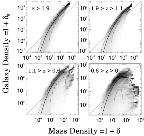
Figure 3: Galaxy mass density as a function of dark matter density for each age quartile, at 1 $h^{-1}$ Mpc radius top hat smoothing. Each panel lists the range of formation redshifts included. Shading is a logarithmic stretch of the conditional probability $P(1+\delta_{g}|1+\delta)$. Solid lines indicate $\left\langle 1+\delta_{g}|1+\delta\right\rangle$; dotted lines indicate the 1$\sigma$ deviation from the mean.

The resulting bias relationship is nonlinear, stochastic, and is a strong function of galaxy age. These properties are revealed in Figure 3, which shows as a greyscale the conditional probability $P(1+\delta_{g}|1+\delta)$ and as the solid line the conditional mean $\left\langle 1+\delta_{g}|1+\delta\right\rangle$, where all quantities are defined with a top hat filter of radius 1 $h^{-1}$ Mpc. Each panel shows the results at $z=0$ for galaxies formed at different epochs, as labeled. Note that the oldest galaxies are the cleanest tracers of the dark matter distribution: the scatter around the mean galaxy-mass relation is small. However, the youngest galaxies show a nonlinear, even non-monotonic, relation with the dark matter; they are under-represented in the very densest regions of the dark matter map (reminiscent of spirals in the cores of clusters, although in the real universe clusters still represent appreciable overdensities in the distribution of late-type galaxies; Strauss et al. 1992). Also, the scatter around the mean density relation for the youngest galaxies is large. In these simulations, the relationship between galaxies and mass also depends on scale. In Figure 4, we show the bias $b\equiv\sigma_{g}/\sigma$ calculated on various scales. The obvious scale-dependence of $b$ is due to the dependence of the galaxy formation process on temperature. The temperature sets the local Jeans mass, which partly determines whether star-formation occurs: the higher the temperature, the greater the overdensity needed to form stars. On small scales the temperature is proportional to the gravitational potential $\phi$. Note that in Fourier space, ${\tilde{\phi}}(k)\propto{\tilde{\delta}}(k)/k^{2}$. For high $k$, then, there is little power in the potential or temperature fields; i.e. these fields are smoother than the density field. Thus, temperature correlates over large scales; furthermore, on these large scales it correlates with density as well. Thus the dependence of galaxy formation on temperature can couple the galaxy density on small scales with the dark matter density on larger scales. As Blanton et al. (1998) show, this coupling causes scale-dependence of the bias relation. The dependence of galaxy formation on local gas temperature is likely to be important in any galaxy formation scenario; thus, this scale-dependence may be generic.

Figure 4: The bias $b(R)\equiv\sigma_{g}(R)/\sigma(R)$, where $R$ refers to the top hat smoothing radius. Solid line indicates all galaxies. Dashed lines indicate each age quartile, with range of formation redshifts listed. Note the strong scale-dependence, and that old galaxies are more biased than young.

The work ahead is evaluate the consequences of this complicated bias relationship for statistical measures of large-scale structure. The data definitely allow stochasticity; in the POTENT-IRAS comparison of Sigad et al. (1998), although the value of $\chi^{2}$/dof is consistent with deterministic bias, it is also consistent with the inclusion of the rms value of $\epsilon$ found in the simulations at 1200 $\rm\,km\ s^{-1}$ smoothing. Moreover, nonlinear relative bias between galaxies of different types is unambiguously observed, in the form of the morphology-density relation (cf. the discussion in Strauss & Blanton 1998). We are in the process of carrying out simulations using realistic bias laws, to determine how it may skew the results of the various analyses described above.

References

- [1] Aaronson, M., et al. 1982, ApJS, 50, 241
- [2] Bertschinger, E., Dekel, A., Faber, S. M., Dressler, A., & Burstein, D. 1990, ApJ, 364, 370
- [3] Blanton, M., Cen, R., Ostriker, J.P., & Strauss, M.A. 1998, ApJ, submitted (astro-ph/9807029)
- [4] da Costa, L. N. et al. 1998, MNRAS, 299, 425
- [5] Davis, M., Efstathiou, G., Frenk, C. S., & White, S. D. M. 1985, ApJ, 292, 371
- [6] Davis, M., Nusser, A., & Willick, J. A. 1996, ApJ, 473, 22
- [7] Dekel, A. 1994, ARA&A, 32, 371
- [8] Dekel, A., Bertschinger, E., & Faber, S. M. 1990, ApJ, 364, 349
- [9] Dekel, A., & Lahav, O. 1998, preprint, astro-ph/9806193
- [10] Dekel, A., & Rees, M. J. 1994, ApJ, 422, L1
- [11] Dekel, A. et al. 1998, in preparation
- [12] Djorgovski, S., & Davis, M. 1987, ApJ, 313, 59
- [13] Dressler, A. et al. 1987, ApJ, 313, 42
- [14] Fisher, K. B. et al. 1995, ApJS, 100, 69
- [15] Freudling, W. et al. 1998, ApJ, submitted
- [16] Giovanelli, R. et al. 1998a, ApJ, 505, L91
- [17] Giovanelli, R. et al. 1998b, AJ, in press (astro-ph/9808158)
- [18] Gunn, J. E., & Oke, J. B. 1975, ApJ, 195, 255
- [19] Hamilton, A.J.S. 1998, in Ringberg Workshop on Large-Scale Structure, ed. D. Hamilton (Kluwer, Amsterdam), 185
- [20] Hamuy, M., Phillips, M.M., Suntzeff, N.B., Schommer, R.A., Maza, J., & Aviles, R. 1996, AJ, 112, 2391
- [21] Haynes, M.P. et al. 1998, in preparation
- [22] Hermit, S., Lahav, O., Santiago, B.X., Strauss, M.A., Davis, M., Dressler, A., & Huchra, J.P. 1996, MNRAS, 283, 709
- [23] Hudson, M. 1993, MNRAS, 265, 43
- [24] Hudson, M. J., Dekel, A., Courteau, S., Faber, S. M., & Willick, J. A. 1995, MNRAS, 274, 305
- [25] Jacoby, G. H. et al. 1992, PASP, 104, 599
- [26] Kaiser, N. 1984, ApJ, 284, L9
- [27] Kolatt, T., & Dekel, A. 1997, ApJ, 479, 592
- [28] Kolatt, T., Dekel, A., Ganon, G., & Willick, J. A. 1996, ApJ, 458, 419
- [29] Lauer, T. R., & Postman, M. 1994, ApJ, 425, 418
- [30] Nusser, A., & Dekel, A. 1993, ApJ, 405, 437
- [31] Phillips, M. M. 1993, ApJ, 413, L105
- [32] Postman, M. 1995, in Dark Matter, Proceedings of the 5th Maryland Astrophysics Conference, AIP Conference Series 336, 371
- [33] Postman, M., & Lauer, T. R. 1995, ApJ, 440, 28
- [34] Riess, A., Press, W., & Kirshner, R. P. 1995, ApJ, 445, L91
- [35] Riess, A., Press, W., & Kirshner, R. P. 1996, ApJ, 473, 88
- [36] Shaya, E. J., Peebles, P. J. E., & Tully, R. B. 1995, ApJ, 454, 15
- [37] Sigad, Y., Eldar, A., Dekel, A., Strauss, M.A., & Yahil, A. 1998, ApJ, 495, 516
- [38] Strauss, M.A. 1997, in Critical Dialogues in Cosmology, edited by Neil Turok (Singapore: World Scientific), 423
- [39] Strauss, M.A., & Blanton, M. 1998, in Astrophysics with Infrared Surveys: A Prelude to SIRTF, edited by M. Bicay (Astronomical Society of the Pacific Conference Series), in press (astro-ph/9809023)
- [40] Strauss, M. A., Davis, M., Yahil, A., & Huchra, J. P. 1992, ApJ, 385, 421
- [41] Strauss, M. A., & Willick, J. A. 1995, Phys. Rep., 261, 271 (SW)
- [42] Teerikorpi, P. 1997, ARA&A, 35, 101
- [43] Tonry, J.L., Blakeslee, J.P., Ajhar, E.A., & Dressler, A. 1997, ApJ, 475, 399
- [44] Tonry, J. L., & Schneider, D. P. 1988, AJ, 96, 807
- [45] Tully, R. B. 1987, Nearby Galaxies Catalog (Cambridge: Cambridge University Press)
- [46] Tully, R. B., & Fisher, J. R. 1977, A&A, 54, 661 (TF)
- [47] Willick J.A. 1998, in Formation of Structure in the Universe, edited by A. Dekel and J.P. Ostriker (Cambridge: Cambridge University Press), in press
- [48] Willick, J. A., Courteau, S., Faber, S. M., Burstein, D., & Dekel, A. 1995, ApJ, 446, 12
- [49] Willick, J. A., Courteau, S., Faber, S. M., Burstein, D., Dekel, A., & Kolatt, T. 1996, ApJ, 457, 460
- [50] Willick, J. A., Courteau, S., Faber, S. M., Burstein, D., Dekel, A., & Strauss, M. A. 1997a, ApJS, 109, 333
- [51] Willick, J.A., & Strauss, M.A. 1998, ApJ, 507, in press
- [52] Willick, J.A., Strauss, M.A., Dekel, A., & Kolatt, T. 1997b, ApJ, 486, 629
- [53] Yahil, A., Strauss, M. A., Davis, M., & Huchra, J. P. 1991, ApJ, 372, 380
- [54] Zaroubi, S., Zehavi, I., Dekel, A., Hoffman, Y., & Kolatt, T. 1997, ApJ, 486, 21
- [55] Zehavi, I., Riess, A.G., Kirshner, R.P., & Dekel. A. 1998, ApJ, 503, 483