Nonlinear Cosmological Structure Formation

Abstract

I present a general discussion of the evolution and model-dependence of both the linear and nonlinear power spectrum of density fluctuations. The features of the linear power spectrum in cosmological models with cold dark matter (CDM) and cold+hot dark matter (C+HDM) are reviewed, and useful analytical approximations are summarized. Cosmological numerical simulation results are then used to illustrate the process of nonlinear gravitational clustering and to compute the nonlinear power spectrum. A new analytical approximation relating the linear and nonlinear power spectrum in C+HDM models is presented.

1 Introduction

The power spectrum $P(k)$ of matter fluctuations is a fundamental quantity in cosmology. It provides the most basic statistical measure of gravitational clustering, and an accurate determination of the power spectrum is among the most important goals of every major galaxy survey. Since each cosmological model has its distinct power spectrum, one can hope to obtain crucial information such as the matter content of the Universe and the nature of the primordial fluctuations by comparing the observed power spectrum with theoretical predictions for various plausible models.

Measurements of the power spectrum require extensive galaxy surveys covering a large volume of space. It is only recently that such surveys have been completed and are starting to reveal intriguing results. For instance, much interest has been generated by the compilation of the power spectrum determined from the APM and IRAS galaxy catalogs and the effort to reconstruct the underlying linear mass power spectrum (Peacock & Dodds 1994; Peacock 1997). The recently completed Las Campanas survey of over 23,000 galaxies has yielded a power spectrum incompatible with the standard cold dark matter (CDM) model but still consistent with a class of open CDM, cold+hot dark matter (C+HDM), and tilted CDM models (Lin et al. 1996). Larger ongoing projects such as the CfA Century, the 2dF, and the Sloan surveys promise to provide measurements with reduced error bars and data points on larger scales for better constraints.

On the theoretical side, calculations of the power spectrum falls into two regimes: the linear and the nonlinear, which are characterized by the amplitude of the density fluctuations $\delta=\delta\rho/\rho\ll 1$ and $>1$, respectively. Since the observed power spectrum spans both linear and nonlinear regimes, theoretical calculations in both regimes must be performed before all data points can be fully utilized as constraints. In the linear regime, the computation of the power spectrum has become standard practice. It is obtained by integrating the coupled, linearized Einstein and Boltzmann equations that describe the evolution of the metric and density perturbations throughout the history of the Universe. Several groups have written numerical codes for such calculations, and a publicly-available version is described in Ma & Bertschinger (1995) and placed at http://arcturus.mit.edu. This code computes, in both synchronous and conformal Newtonian gauges, the evolution of the phase-space distributions of photons, baryons, cold dark matter, and both massless and massive neutrinos. It is therefore applicable to most CDM, C+HDM, and CDM with a cosmological constant (LCDM) models. To gain deeper insight and for convenience, analytical approximations for the linear power spectra in these models have also been published. Details about the linear power spectrum are discussed in Section 2.

Gravitational clustering, however, eventually becomes a nonlinear process. The existence of galaxies and clusters is a manifestation of the nonlinear nature of gravity. Determining the nonlinear power spectrum $P_{\rm nl}$ is therefore an important task. Not surprisingly, $P_{\rm nl}$ is more difficult to obtain than the linear power spectrum. Higher-order perturbation theories help to extend the range of validity to the quasi-linear regime, but the fully nonlinear power spectrum can be calculated only from numerical simulations. Thus far, theoretical predictions of $P_{\rm nl}$ have been carried out for only a few models at limited epochs because it is difficult and time-consuming to perform numerical simulations with sufficient dynamic range to allow calculations of $P_{\rm nl}$ over a wide range of scales. Section 3 summarizes some recent work and presents new analytic and numerical results for nonlinear clustering in C+HDM models.

2 Linear Power Spectrum

The power spectrum $P(k)$ of matter fluctuations is related to the density field $\delta$ in $k$-space by

$$\left<\delta(\vec{k})\delta^{*}(\vec{k}^{\prime})\right>=P(k)\delta_{D}(\vec{k}-\vec{k}^{\prime})\,,$$ (1)

where $\delta_{D}$ is the Dirac-delta function. The Fourier transform of the power spectrum is the two-point correlation function $\xi(r)=\left<\delta(\vec{x_{1}})\delta(\vec{x_{2}})\right>$, where $r\equiv|\vec{x_{1}}-\vec{x_{2}}|$. For a Gaussian density field (as predicted in most inflationary theories), its statistical property is entirely determined by $P(k)$.

The shape of the linear power spectrum depends on the cosmological parameters assumed in a given theory of structure formation. It is governed by the linear perturbation theory of gravitational clustering, and can be computed by integrating the coupled, linearized Einstein, Boltzmann, and fluid equations for the metric and density perturbations. Some important parameters that affect the shape of the power spectrum are: (1) Primordial spectral index $n$: $P(k)\propto k^{n}$. An example is the Harrison-Zeldovich (Harrison 1970; Zeldovich 1972) spectrum which takes $n=1$. Most versions of inflationary models also predict nearly $n=1$ power spectra. (2) Matter-radiation equality time: The equality time $t_{\rm eq}$ is defined to be the epoch in the thermal history of the Universe when the energy density in matter equals that in radiation. The equality redshift scales as $1+z_{\rm eq}\propto\Omega_{\rm m}h^{2}$, where $\Omega_{\rm m}$ is the density parameter in matter and $h$ is the Hubble constant in units of 100 km/s/Mpc. This parameter controls the location of the peak of $P(k)$ in CDM-type models since the density perturbations with wavenumbers $k>k_{\rm eq}$ enter the horizon in the radiation-dominated era and cannot grow appreciably, whereas perturbations with $k<k_{\rm eq}$ enter the horizon in the matter-dominated era and can grow unimpeded. (3) Nature of dark matter. The pure CDM model, for example, exhibits a characteristic $P(k)\propto k^{-3}$ slope at high $k$, while the power spectrum for the pure hot dark matter (HDM) model is cut off exponentially below the free-streaming scale of the massive neutrinos due to the phase mixing in the neutrino phase-space distribution. The hybrid C+HDM models, which are parameterized by the neutrino mass density $\Omega_{\nu}$ and CDM mass density $\Omega_{c}=1-\Omega_{\nu}-\Omega_{b}$ (where $\Omega_{b}$ is the mass density in baryons), exhibit intermediate behavior. The suppression in the power in both the cold and hot components due to neutrino free-streaming generally increases with increasing $\Omega_{\nu}$.

The solid curves in Figure 1 show the linear power spectra for the pure CDM and three C+HDM models with $\Omega_{\nu}=0.1,0.2$, and 0.3. The corresponding neutrino masses in the four models are 0, 2.3, 4.6, and 7 eV, respectively. (Only one of the three species of neutrinos is assumed massive.) The models have a total matter density of $\Omega_{m}=1$ and $h=0.5$, and all are normalized to the COBE rms quadrupole $Q_{\rm rms-PS}=18\,\mu K$ (Gorski et al. 1996), as evidenced by the convergence of the curves at small $k$. The differences at large $k$ reflect the distinct properties of cold and hot dark matter: the larger $\Omega_{\nu}$ is, the weaker is the gravitational clustering on small length scales. For comparison, a COBE-normalized low-density model with $\Omega_{m}=0.3$, a cosmological constant $\Omega_{\Lambda}=0.7$, and $h=0.75$ is also shown (dashed curve).

Analytical approximations with less than $10$% error are very convenient as an input for many calculations. The pure CDM model is well-approximated by

$$P_{c}(q,a,\Omega_{\nu}=0) = A\,a^{2}\,k^{n}$$ (2)

$$\times \left[{\ln(1+\alpha_{1}q)\over\alpha_{1}q}\right]^{2}{1\over[1+\alpha_{2}q+(\alpha_{3}q)^{2}+(\alpha_{4}q)^{3}+(\alpha_{5}\,q)^{4}]^{1/2}}\,,\quad q={k\over\Gamma h}\,,$$

where $A$ is the overall normalization factor, $a$ is the expansion factor, $n$ is the primordial spectral index, $k$ is the wavenumber in units of Mpc^-1, and $\alpha_{1}=2.34,\alpha_{2}=3.89,\alpha_{3}=16.1,\alpha_{4}=5.46$, and $\alpha_{5}=6.71$ (Bardeen et al. 1986). The normalization $A$ can be determined from the 4-year data from the COBE satellite, and $A=2420\,h^{-4}$ Mpc⁴ for $n=1$ flat models (Bunn & White 1997). The shape parameter $\Gamma$ characterizes the dependence on cosmological parameters, and a good approximation is found to be given by $\Gamma=\Omega_{\rm m}h/\exp[\Omega_{\rm b}(1+1/\Omega_{\rm m})]$ (Efstathiou et al. 1992; Sugiyama 1995). The error in the approximation for the standard CDM model with $\Omega_{\rm b}=0.05$, for example, is $<10$%. A higher-accuracy fit for this much-studied model can be achieved by setting $\Omega_{\rm b}=0$ in equation (2) (i.e. setting $\Gamma=\Omega_{\rm m}h$) and modifying the coefficients to $\alpha_{1}=2.205,\alpha_{2}=4.05,\alpha_{3}=18.3,\alpha_{4}=8.725$, and $\alpha_{5}=8.0$. The fractional error relative to the direct numerical result is then reduced to smaller than 1% for $k<40\,h$ Mpc^-1 (Ma 1996).

The linear power spectra for the C+HDM models require additional treatment since the effect of neutrino free-streaming on the shape of the power spectrum is both time- and scale-dependent. It is found (Ma 1996) that by introducing a second shape parameter

$$\Gamma_{\nu}=a^{1/2}\Omega_{\nu}h^{2}$$ (3)

to characterize the neutrino free-streaming distance, accurate approximations to the linear power spectra in C+HDM models can be obtained. The cold and hot components clearly have different power spectra due to their different thermal properties. For the CDM component in C+HDM models, a good approximation is given by

$$P_{c}(k,a,\Omega_{\nu})=P_{c}(k,a,\Omega_{\nu}=0)\left({1+b_{1}\,x^{b_{4}/2}+b_{2}\,x^{b_{4}}\over 1+b_{3}\,x_{0}^{b_{4}}}\right)^{\Omega_{\nu}^{1.05}}\,,\quad x={k\over\Gamma_{\nu}}\,,\quad x_{0}=x(a=1)\,,$$ (4)

where $P_{c}(k,a,\Omega_{\nu}=0)$ for the pure CDM model is given by equation (2), and $b_{1}=0.01647,b_{2}=2.803\times 10^{-5},b_{3}=10.90$, and $b_{4}=3.259$ for $k$ in units of Mpc^-1. The functional form for the ratio $P_{c}(k,a,\Omega_{\nu})/P_{c}(k,a,0)$ is chosen to have the asymptotic behavior $\propto a^{2(f_{\infty}-1)}$, which can be derived analytically, and $f_{\infty}=(5\sqrt{1-24\Omega_{\nu}/25}-1)/4$ is the asymptotic growth rate for $k\rightarrow\infty$, where $1-f_{\infty}\propto\Omega_{\nu}^{1.05}$ is a good approximation. For the HDM component in C+HDM models, an accurate approximation is given by

$$P_{\nu}(k,a,\Omega_{\nu})=P_{c}(k,a,\Omega_{\nu})\left({e^{-c_{1}\,x}\over 1+c_{2}\,x^{1/2}+c_{3}\,x+c_{4}\,x^{3/2}+c_{5}\,x^{2}}\right)\,,\quad x={k\over\Gamma_{\nu}\,h}\,,$$ (5)

where $c_{1}=0.0015,c_{2}=-0.1207,c_{3}=0.1015,c_{4}=-0.01618$, and $c_{5}=0.001711$ for $k$ in units of Mpc^-1.

It is often useful to have an analytic approximation for the density-weighted power spectrum $P(k)=\{\Omega_{\nu}P_{\nu}^{1/2}+(1-\Omega_{\nu})P_{c}^{1/2}\}^{2}$ that measures the total gravitational fluctuations contributed by the two components. Here the CDM and baryons have been assumed to have the same power (i.e., $P_{c}=P_{b}$), which is a good approximation for the range of redshifts and $\Omega_{b}$ studied in this paper. The functional form used for the CDM spectrum $P_{c}$ in equation (4) works well here, and a good approximation for the density-weighted power spectrum in C+HDM models is given by

$${P(k,a,\Omega_{\nu})\over P_{c}(k,a,\Omega_{\nu}=0)}=g(x,\Omega_{\nu})=\left({1+d_{1}\,x^{d_{4}/2}+d_{2}\,x^{d_{4}}\over 1+d_{3}\,x_{0}^{d_{4}}}\right)^{\Omega_{\nu}^{1.05}}\,,\quad x={k\over\Gamma_{\nu}}\,,\quad x_{0}=x(a=1)\,,$$ (6)

where $P_{c}(k,a,\Omega_{\nu}=0)$ again is given by equation (2), and the coefficients are $d_{1}=0.004321,d_{2}=2.217\times 10^{-6},d_{3}=11.63$, and $d_{4}=3.317$ for $k$ in units of Mpc^-1.

It should be noted that the C+HDM power spectra do not obey the simple evolution $P(k)\propto a^{2}$ in equation (2) for the flat pure CDM model. The free-streaming of massive neutrinos slows down with time, allowing the neutrinos to cluster gravitationally and the neutrino density perturbations to grow on increasingly smaller scales. As a result, the growth of the C+HDM power spectra is both scale- and time-dependent. This effect is taken care of by the time-dependent parameter $\Gamma_{\nu}$ in equation (3), which is built in in equations (4)-(6) via the scaled variable $x$.

3 Nonlinear Gravitational Clustering

3.1 Numerical Simulations

The linear theory of gravitational clustering is an elegant and powerful theory. It describes accurately the growth of density perturbations from the early Universe until a redshift of $\sim 100$, and the solution to the theory involves straightforward time-integration of a set (albeit a large set) of coupled ordinary differential equations. Gravitational clustering, however, eventually becomes a nonlinear process, and the study of the fully nonlinear process ultimately relies on numerical simulations.

Cosmological simulations can be roughly divided into two categories: (1) $N$-body simulations that deal only with dissipationless gravitational interactions of dark matter; and (2) hydrodynamical simulations that model gaseous dissipation via cooling and heating processes in addition to the gravitational interactions among the dark matter and gas. Depending on the models, the simulations are started at a redshift between 20 and 100 when the rms density fluctuations are well below unity, and the initial conditions of the simulations are generated from the linear power spectrum at that epoch.

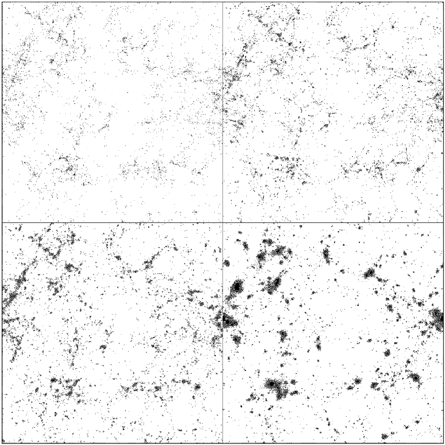
Figure 2: The smoothed matter distribution at four redshifts, $z=5$ (upper left), 3 (upper right), 1.5 (lower left), and 0 (lower right), from an $N$-body simulation of the $\Omega_{\nu}=0.1$ C+HDM model. Each panel is 100$\times$100 Mpc comoving, and shows projection along one axis of the entire simulation box.

As an illustration of gravitational clustering in collisionless $N$-body simulations, Figure 2 shows the projection of the smoothed matter distribution at four redshifts, $z=5,3,1.5$, and 0, from an $N$-body simulation of the $\Omega_{\nu}=0.1$ C+HDM model. The model assumes $\Omega_{c}=0.85$, $\Omega_{\rm b}=0.05$, and $h=0.5$, and is normalized to the COBE quadrupole $Q_{\rm rms-PS}=18\,\mu K$ (Gorski et al. 1996). The simulation box is 100 Mpc comoving on a side, and the force softening is 50 kpc. A total of $128^{3}$ cold and $128^{3}$ hot particles are used. Each panel in Figure 2 is 100$\times$100 Mpc comoving, and shows the projection along one axis of the entire simulation box. Periodic boundary conditions are adopted in the simulation, so for example, the dense clumps near the central left and right edges of the box in the $z=0$ panel (lower right) are part of the same cluster of dark matter halos. The darkest several halos at $z=0$ all have masses above $10^{14}M_{\odot}$.

The power spectrum of the density fluctuations offers the lowest-order measurement of the gravitational clustering exhibited in Figure 2. In Figure 3, we plot the corresponding nonlinear power spectra computed from the particle spatial distributions at $z=3,1.5$, and 0 shown in Figure 2. The linear power spectra given by equation (6) are also shown for comparison. The hierarchical, or “bottom-up”, nature of gravitational collapse in these models is evident: the high-$k$ modes (i.e. small length scales) have become strongly nonlinear, while the low-$k$ modes are still following the linear power spectrum. The fact that the three lowest $k$ modes are still linear at $z=0$ ensures that our choice of the simulation box size (100 Mpc) is large enough to include all waves that have gone nonlinear at the present epoch. It is also interesting to note that the point of departure from linearity moves to the left of the figure as $z$ decreases, indicating that objects become nonlinear on increasingly larger length scales as the Universe evolves.

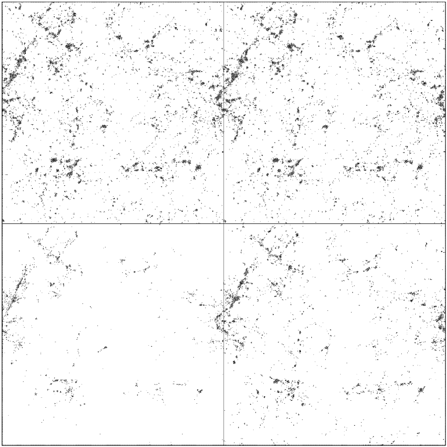
Figure 4: The smoothed matter distribution at $z=1.5$ from $N$-body simulations of four cosmological models: LCDM with $\Omega_{\rm m}=0.3$ and $\Omega_{\Lambda}=0.7$, and C+HDM with $\Omega_{\nu}=0.1,0.2$, and 0.3 (clockwise from upper left). Each panel is 100$\times$100 Mpc comoving, and shows projection along one axis of the entire simulation box. The same initial random phases were used in all four simulations, so structures appear in similar locations in all panels.

It is also instructive to compare the nonlinear structures at the same epoch in different cosmological models. Figure 4 shows the smoothed matter distribution at $z=1.5$ from simulations of the four models in Figure 1: a LCDM, and C+HDM with $\Omega_{\nu}=0.1,0.2$, and 0.3 (clockwise starting from upper left). The LCDM model has $\Omega_{\rm m}=0.3$, $\Omega_{\Lambda}=0.7$, and $h=0.75$, and the three C+HDM models have $h=0.5$, $\Omega_{\rm b}=0.05$, and $\Omega_{c}+\Omega_{\nu}+\Omega_{\rm b}=1$. All models are COBE-normalized, and all simulations are performed with the same box size and force resolution as the $\Omega_{\nu}=0.1$ run described earlier. (The only exception is that the $\Omega_{\nu}=0.2$ and 0.3 simulations used $10\times 128^{3}$ instead of $128^{3}$ particles to represent the HDM component.) The initial conditions for all four simulations are generated with the same random phases; structures therefore appear at similar locations in all panels. The effect of $\Omega_{\nu}$ on structure formation, however, is striking: the higher $\Omega_{\nu}$ is, the fewer collapsed objects there are at a given epoch. This trend simply reflects the decrease in the small-scale linear power shown in Figure 1, which results from neutrino free-streaming. Note that the model with $\Omega_{\nu}=0.3$ (lower left panel), which corresponds to a neutrino mass of 7 eV, has very few structures even at $z=1.5$. It is also interesting to note that the upper two panels of Figure 4 for the LCDM and $\Omega_{\nu}=0.1$ C+HDM models look very similar. This is because the linear power spectra for the two models are in fact very similar at $k>0.1\,h$ Mpc^-1, as shown in Figure 1. The corresponding linear and nonlinear power spectra at $z=1.5$ for the three C+HDM models in Figure 4 are shown in Figure 5.

The power spectra shown thus far for the C+HDM models are the density-averaged $P(k)=\{\Omega_{\nu}\,P_{\nu}^{1/2}+(1-\Omega_{\nu})\,P_{c}^{1/2}\}^{2}$, where $P_{\nu}$ and $P_{c}$ are the individual power spectra for the hot and cold components. (It has been assumed $P_{c}=P_{\rm baryon}$, which is a good approximation for the redshift range of interest here.) The two components evolve distinctly due to their different thermal velocities, and the details of the shape and the growth of the linear power spectra are discussed in Ma (1996). Here, the nonlinear power spectra for the separate components are presented in Figure 6. For clarity, only two epochs, $z=3$ and 0, are plotted. Notice how at $z=3$, the HDM spectrum remains linear to almost $k=2\,h\,$Mpc^-1 but the CDM remains linear to only $k\sim 0.5\,h$Mpc^-1, while at $z=0$, both components become nonlinear at $k\approx 0.3\,h\,$Mpc^-1. This is largely due to the slowing down of the neutrinos, which makes it easier for the neutrino particles to fall into the CDM potential wells at later times, and therefore become nonlinear at smaller $k$. More precisely, the median thermal velocity of neutrinos is

$$v\approx 3(1+z){k_{B}T_{0,\nu}\over m_{\nu}c}=15(1+z){10\,{\rm eV}\over m_{\nu}}\,{\rm km/s}\,,$$ (7)

so the neutrinos in the $\Omega_{\nu}=0.1$ model ($m_{\nu}=2.3$ eV) have slowed down by a factor of 4 since $z=3$ to about 60 km/s today.

3.2 Analytical Approximations

Just as it was useful to cast the linear power spectra in simple functional forms for a wide range of models (see equations (1)-(6)), analytical approximations to the nonlinear power spectrum can also provide valuable insight to the process of gravitational clustering. It is, however, more difficult to compute the nonlinear $P_{\rm nl}$ because the numerical simulations that have sufficient dynamic range to allow calculations of $P_{\rm nl}$ over a wide range of scales are generally much more CPU-intensive than the integration of the linearized Boltzmann equations. The behavior of the power spectrum in the nonlinear regime therefore is less well-understood.

An early attempt to relate linear and nonlinear quantities was focused on the spatially-averaged two-point correlation function $\bar{\xi}(r)$ in models with $\Omega_{\rm m}=1$ and a power-law power spectrum (Hamilton et al. 1991). It was found that if a given nonlinear scale $r_{\rm nl}$ is identified with its pre-collapsed linear scale $r_{\rm l}$ by $r_{\rm l}^{3}=r_{\rm nl}^{3}(1+\bar{\xi}_{\rm nl})$, then there exists a simple, universal function relating the linear and nonlinear two-point correlation function:

$$\bar{\xi}_{\rm nl}(r_{\rm nl})=F[\bar{\xi}_{\rm l}(r_{\rm l})]\,.$$ (8)

At that time, this transformation appeared to be magically independent of the spectral index $n$ of the linear power spectrum assumed in the model, and the generality of this formula rendered the task of reconstructing the primordial spectrum from the observed nonlinear clustering of galaxies less complicated. However, further tests against numerical simulations showed that this formula worked well only for spectral index $n>-1$, and it erred by factors up to 3 and 10 for $n=-1.5$ and $-2$, respectively (Jain et al. 1995). In particular, the nonlinear $\bar{\xi}_{\rm nl}$ was found to rise more sharply with increasing $\bar{\xi}_{\rm l}$ for models with more negative $n$, so Jain et al. introduced an $n$-dependent formula to accommodate this feature. For the more realistic cosmological models such as the CDM where the spectral index is a function of scale, they proposed to use an effective index $n_{\rm eff}$, defined to be $n_{\rm eff}=d\ln P/d\ln k_{0}$, where $k_{0}$ is the scale at which the rms mass fluctuation $\sigma(R=1/k_{0})$ is unity. The index $n_{\rm eff}$ therefore represents the slope of the power spectrum at a scale where nonlinear effects are becoming important. Later work extended the analysis to models with varying matter density $\Omega_{\rm m}$ and cosmological constant $\Omega_{\Lambda}$ (Peacock & Dodds 1996), where instead of using an effective index for all scales, the local slope $n(k)=d\ln P/d\ln k$ was adopted.

Here we examine the nonlinear mapping of the power spectrum in the C+HDM models, which has not been explored yet. Figure 7 shows how the nonlinear density variance $\Delta_{\rm nl}=4\pi k_{\rm nl}^{3}\,P_{\rm nl}(k_{\rm nl})$ diverges from the linear $\Delta_{\rm l}=4\pi k_{\rm l}^{3}\,P_{\rm l}(k_{\rm l})$, where the linear and nonlinear wavenumbers are related by $k_{\rm l}^{3}=k_{\rm nl}^{3}/(1+\Delta_{\rm nl})$. The squares are obtained from simulations of the $\Omega_{\nu}=0.2$ (left curve) and 0.1 (right) C+HDM models. The curves generally obey the asymptotic condition $\Delta_{\rm nl}=\Delta_{\rm l}$ for $\Delta_{\rm l}\ll 1$, and $\Delta_{\rm nl}\propto\Delta_{\rm l}^{1.5}$ in the highly-nonlinear, stable clustering regime. The mapping, however, is clearly not independent of cosmology: the larger $\Omega_{\nu}$ is in a model, the faster $\Delta_{\rm nl}/\Delta_{\rm l}$ increases at $\Delta_{\rm l}\sim 1$. This trend reflects the $n$-dependence pointed out by Jain et al. (1995) and can be explained by the different shapes of $P_{\rm l}$ shown in Figure 1, where the models with higher $\Omega_{\nu}$ have less power and hence more negative slope at high $k$. Since all models are normalized to COBE and have the same amplitude at low $k$, the critical $k_{0}$ (where $\sigma(k_{0})=1$) increases for larger $\Omega_{\nu}$. The effective index $n_{\rm eff}$ defined at $k_{0}$ is therefore more negative for larger $\Omega_{\nu}$, resulting in the steeper rise of $\Delta_{\rm nl}$ in Figure 7.

However, neither formula proposed by Jain et al. (1995) or Peacock & Dodds (1996) can be extended to the C+HDM models. The dotted curves in Figure 7 illustrate the large discrepancies in the Peacock-Dodds fitting function when it is applied to the $\Omega_{\nu}=0.1$ and 0.2 models. In retrospect, it is not surprising their formulas do not apply: Although the power spectrum at a given epoch is determined entirely from the spatial distribution of the particles, the evolution of the power spectrum depends on the particle velocities as well. A general formula for the linear to nonlinear transformation therefore must depend on both the shape and the growth rate of $P(k)$. Since both formulas are designed for models without massive neutrinos and depend only on the shape of $P(k)$, they cannot be applied to C+HDM models.

Here we propose a new analytical approximation for the mapping of linear and nonlinear power spectrum in CDM as well as C+HDM models:

$$\Delta_{\rm nl}(k_{\rm nl})=\Delta_{\rm l}(k_{\rm l})G\left[{\Delta_{l}}(k_{\rm l})\right]\,,$$ (9)

where

$$G(x)={1+a_{1}x^{4}+a_{2}x^{8}/g^{2.5}\over 1+a_{3}x^{4}+a_{4}x^{7.5}/g^{2}}\,,$$ (10)

and the coefficients are $a_{1}=4756,a_{2}=384.6,a_{3}=3732$, and $a_{4}=24.20$. The functional form of $G$ is chosen to give the appropriate asymptotic behavior $\Delta_{\rm nl}\rightarrow\Delta_{\rm l}$ in the linear regime ($x\ll 1$) and $\Delta_{\rm nl}\propto\Delta_{\rm l}^{3/2}$ in the stable clustering regime ($x\gg 1$). The dependence of $G$ on $\Omega_{\nu}$ comes from the function $g$ of equation (6), which gives the relative amplitudes of the power spectra in the C+HDM models and the pure CDM model. This function is analogous to the commonly-used growth factor $g(a=1,\Omega_{\rm m},\Omega_{\Lambda})={5\over 2}\Omega_{\rm m}[\Omega_{\rm m}^{4/7}-\Omega_{\Lambda}+(1+\Omega_{\rm m}/2)(1+\Omega_{\Lambda}/70)]^{-1}$ for LCDM models (Lahav et al. 1991; Carroll, Press & Turner 1992). They differ, however, in that the growth factor is scale-independent in LCDM models but is a function of scale in C+HDM models since neutrinos only affect the growth below the free-streaming scale, as discussed in Section 2.

4 Summary

The power spectrum is a fundamental measure of gravitational clustering in cosmology. We have discussed the features and evolution of both the linear and nonlinear power spectra in various cosmological models.

The linear power spectrum $P_{l}$ is calculated from time integration of the coupled, linearized Einstein, Boltzmann, and fluid equations for the metric and density perturbations. The shape and growth of the power spectrum depend on cosmological parameters such as the total matter density $\Omega_{\rm m}$, the neutrino fraction $\Omega_{\nu}$, and the Hubble constant $h$. Simple analytical functions were presented that can approximate the linear $P_{l}$ in both CDM and C+HDM models with less than 10% error.

The fully nonlinear power spectrum $P_{\rm nl}$ has to be computed from numerical simulations. Simulation output for CDM, LCDM, and C+HDM models was presented to illustrate the sensitive dependence of structure formation and evolution on cosmological parameters. We also discussed the present understanding of the relation between the linear and nonlinear power spectra, and proposed a new approximation which applies to CDM as well as C+HDM models.

The supercomputing time for this work was generously provided by the National Scalable Cluster Project at the University of Pennsylvania and the National Center for Supercomputing Applications.

Figure 1: The linear power spectrum of density fluctuations at $z=0$ for the standard CDM model (top solid), the C+HDM models with $\Omega_{\nu}=0.1,0.2$, and 0.3 (lower solid), and the LCDM model with $\Omega_{m}=0.3$ and $\Omega_{\Lambda}=0.7$ (dashed). All are COBE-normalized.

Figure 3: The corresponding power spectrum at $z=3,1.5$, and 0 (from bottom up), for the $\Omega_{\nu}=0.1$ C+HDM model shown in Figure 2. The solid curves show the linear $P(k)$ predicted by the linear perturbation theory; the triangles show the nonlinear $P(k)$ computed from the $N$-body simulation.

Figure 5: The matter power spectrum at $z=1.5$ for the three C+HDM models shown in Figure 4. The solid curves show the linear $P(k)$ predicted by the linear perturbation theory; the triangles show the nonlinear $P(k)$ computed from the $N$-body simulations.

Figure 6: The separate CDM and HDM power spectra at $z=3$ (lower set) and 0 (upper set) for the $\Omega_{\nu}=0.1$ C+HDM model. The linear and nonlinear $P(k)$ are shown as solid curves and triangles, respectively. For each pair of curves, the higher one is for the CDM and the lower one for the HDM.

Figure 7: The squares show the ratio of the nonlinear and linear $\Delta(k)=4\pi k^{3}P(k)$ at $z=0$ from the $\Omega_{\nu}=0.2$ (left curve) and 0.1 (right curve) C+HDM simulations. The formula proposed by Peacock & Dodds (1996) for the pure CDM models leads to large errors when applied to the C+HDM models (dotted curves; left for $\Omega_{\nu}=0.2$ and right for 0.1). The solid curves show our improved analytical approximation from equation (10), where the right-most one is for the pure CDM model. (A modified approximation with a higher accuracy than eq. (10) has since appeared in Ma (1998).)

References

- (1) Bardeen, J. M., J. R. Bond, N. Kaiser, & A. S. Szalay. 1986. ApJ 304: 15.
- (2) Bunn, E. & M. White. 1997. ApJ 480: 6.
- (3) Carroll, S., W. Press, & E. L. Turner. 1992. ARAA 30: 499.
- (4) Efstathiou, G., J. R. Bond, & S. D. M. White. 1992. MNRAS 258: 1p.
- (5) Gorski, K. M. et al. 1996. ApJ 464: L11.
- (6) Hamilton, A. J. S., P. Kumar, E. Lu, & A. Matthews. 1991. ApJ 374: L1.
- (7) Harrison, E. R. 1970. Phys. Rev. D. 1: 2726.
- (8) Jain, B., H. J. Mo, & S. D. M. White. 1995. MNRAS 276: L25.
- (9) Lahav, O., P. Lilje, J. Primack, & M. Rees. 1991. MNRAS 251: 128.
- (10) Lin, H. et al. 1996. ApJ 471: 617.
- (11) Ma, C.-P., & E. Bertschinger. 1995. ApJ 455: 7.
- (12) Ma, C.-P. 1996. ApJ 471: 13.
- (13) Ma, C.-P. 1998. ApJL 508: in press (astro-ph/9809267).
- (14) Peacock, J. A. 1997. MNRAS 284: 885.
- (15) Peacock, J. A., & S. J. Dodds. 1994. MNRAS 267: 1020.
- (16) Peacock, J. A., & S. J. Dodds. 1996. MNRAS 280: L19.
- (17) Sugiyama, N. 1995. ApJS 100: 281.
- (18) Zeldovich, Ya. B. 1972. MNRAS 160: 1p.