Nucleosynthesis in Type II supernovae and
the abundances in metal-poor stars

Abstract

We explore the effects on nucleosynthesis in Type II supernovae of various parameters (mass cut, neutron excess, explosion energy, progenitor mass) in order to explain the observed trends of the iron-peak element abundance ratios ([Cr/Fe], [Mn/Fe], [Co/Fe] and [Ni/Fe]) in halo stars as a function of metallicity for the range $-4\leq$ [Fe/H] $\leq-2.5$. [Cr/Fe] and [Mn/Fe] decrease with decreasing [Fe/H], while [Co/Fe] behaves the opposite way and increases. We show that such a behavior can be explained by a variation of mass cuts in Type II supernovae as a function of progenitor mass, which provides a changing mix of nucleosynthesis from an alpha-rich freeze-out of Si-burning and incomplete Si-burning. This explanation is consistent with the amount of ejected ⁵⁶Ni determined from modeling the early light curves of individual supernovae. We also suggest that the ratio [H/Fe] of halo stars is mainly determined by the mass of interstellar hydrogen mixed with the ejecta of a single supernova which is larger for larger explosion energy and the larger Strömgren radius of the progenitor.

1. INTRODUCTION

Very metal poor stars provide important clues to investigate early Galactic chemical and dynamical evolution because they contain valuable information about this time. We can learn how the Galaxy evolved chemically (as well as dynamically) in its early phase from the observation of these stars. Therefore, a large number of observations and abundance analyses have been performed. Until recently, no significant abundance change with metallicity had been observed. However, recent high-resolution abundance surveys have discovered interesting trends of [Cr/Fe], [Mn/Fe] and [Co/Fe] with respect to [Fe/H] ([A/B] = log₁₀(A/B)$-$log₁₀(A/B)_⊙). Both [Cr/Fe] and [Mn/Fe] decrease with decreasing metallicity from [Fe/H] = $-2.4$ to $-4.0$, while [Co/Fe] increases (Figure 1) (McWilliam et al. 1995a, 1995b; McWilliam 1997; see also Ryan et al. 1996 and reference therein).

Over the last few years, these trends have been the subject of controversy. McWilliam et al. (1995b) discussed the time-delay mechanism, which produces the abundance trends by the time-delay between SNe II with different masses or between SNe I and SNe II. They argued that this mechanism works for several species such as $\alpha$-elements but has difficulties with the above trends. McWilliam et al. (1995b) also pointed out that the Galactic halo formation model proposed by Searle & Zinn (1978) is at odds with the time-delay mechanism. Instead, they suggested that the metallicity-dependent supernova progenitor mass function could explain these trends, while still being consistent with Searle & Zinn (1978). Audouze & Silk (1995) interpreted the observations as evidence that the Galaxy was poorly mixed and proposed that at most two or three supernovae could have contaminated any particular cloud. In favor of this hypothesis, Ryan et al. (1996) proposed that a variation of the supernova explosion energy, which is connected with both the yields and the amount of ejecta dilution, could cause these trends. McWilliam (1997) and Searle & McWilliam (1998) suggested that diluting a primordial composition with solar composition supernova ejecta could explain the trends. In principle, hypothetical pre-galactic population III objects, such as very massive stars or pair creation supernovae (e.g., Bond et al. 1984), could be the cause of the observed behavior. However, none of these objects has been investigated in full detail in quantitative nucleosynthesis yield studies nor ever been incorporated in chemical evolution calculations.

Timmes et al. (1995) constructed a Galactic evolution model using a grid of Type II supernova models (Woosley & Weaver 1995, hereafter WW95), but did not explain the above-mentioned abundance trends. In Timmes et al. (1995), only the region with [Fe/H] $>-3.0$ was investigated, so that only limited information is available. However, their results seem to suggest that the metallicity effect alone cannot explain the observed trends.

The purpose of this paper is to provide a qualitative explanation of the halo abundance data within the framework of Type II supernovae (SNe II) explosive nucleosynthesis. It should be pointed out that self-consistent explosion and nucleosynthesis calculations, which start from core collapse, have not yet successfully determined the mass cut between the central neutron star (or black hole) and the ejected envelope. Therefore, the mass cut of SNe II as a function of the progenitor mass is still an open question and can be treated as a free parameter. This investigation focuses on the mass cut, which determines the amount of ⁵⁶Ni in SN II ejecta, and its possible connection with the amount of (stable) Cr, Mn, Co, and Ni ejected. The connection between stellar evolution, explosive yields, and galactic evolution, observed via abundances in low metallicity stars, is made by performing chemical evolution studies in the framework previously described by Tsujimoto et al. (1995, 1997).

Although we are investigating the nucleosynthesis of low-metallicity stars, we use solar metallicity pre-supernova models in this paper for the following reasons. Previously, only WW95 calculated nucleosynthesis of SNe II using progenitor models with low metallicities; however, their progenitor models have not yet been published. Their results suggest that although the yields of iron peak elements depend on the progenitor metallicity, their variation in the range $Z=(10^{-2}-10^{-4})Z_{\odot}$ is only about 20% or less. Since we are interested only in $Z$ in this range, we neglect metallicity effects on progenitors and explore the dependence on other parameters, such as the stellar mass, mass cut, explosion energy, and neutron excess ($=1-2Y_{e}$, where $Y_{e}$ denotes the electron mole number). With this procedure, we can investigate the trends of the yields, i.e., how much the yields increase or decrease with these parameters.

In §2, we review the nucleosynthesis yields of SNe II (including their dependence on the mass cut, explosion energy, and $Y_{e}$ of the innermost ejected matter). The results are applied in chemical evolution calculations in §3 in order to explore whether the observed abundance patterns in the metal-poor stars can be explained with our approach. Section 4 contains a more in-depth discussion, listing both the successes and the remaining open questions.

2. NUCLEOSYNTHESIS IN TYPE II SUPERNOVAE

2.1. Models

Stars initially more massive than 8$M_{\odot}$ explode as SNe II at the end of their life, leaving neutron stars or black holes. When they explode, nucleosynthesis proceeds explosively because of high temperatures and densities in the deep stellar interior. In order to investigate the explosive nucleosynthesis of SNe II, we solve nuclear reaction networks, together with hydrodynamical equations, and calculate the energy generation by explosive burning.

Our calculations are performed in two steps. The first step is a hydrodynamical simulation of the SN II explosions with a small nuclear reaction network which contains only 13 alpha nuclei (⁴He, ¹²C, ¹⁶O, ²⁰Ne, ²⁴Mg, ²⁸Si, ³²S, ³⁶Ar, ⁴⁰Ca, ⁴⁴Ti, ⁴⁸Cr, ⁵²Fe, and ⁵⁶Ni). The hydrodynamical simulations are carried out with a one dimensional PPM (piecewise parabolic method) code (Colella and Woodward 1984). We generate a shock by depositing thermal energy below the mass cut that divides the ejecta and the collapsing core, and perform the induced nucleosynthesis calculations following the procedure of our previous investigations (e.g. Hashimoto et al. 1989; Thielemann, Hashimoto, & Nomoto 1990; Thielemann, Nomoto, & Hashimoto 1996, hereafter TNH96). In the second step, at each mesh point of the hydrodynamical model, post-processing calculations are performed with an extended reaction network (Hix & Thielemann 1996), which contains 211 isotopes, and provides precise total yields (also for minor abundances).

In our calculation, the progenitor models are taken from Nomoto & Hashimoto (1988, hereafter NH88). Figure 2 shows the $Y_{e}$ profiles of the models (25$M_{\odot}$, 20$M_{\odot}$ and 13$M_{\odot}$) in NH88. In this paper, $Y_{e}$ in the deep stellar interior is modified to take a constant value of $Y_{e}^{\rm deep}$ from $M_{\rm r}=M_{\rm cut}$ to $M_{\rm r}=1.70M_{\odot}$ (for the 25$M_{\odot}$ star), $M_{\rm r}=1.64M_{\odot}$ (20$M_{\odot}$ star) and $M_{\rm r}=1.49M_{\odot}$ (13$M_{\odot}$ star). NH88’s $Y_{e}$ distribution of the progenitor is adopted for the outer region above the boundaries shown in Figure 2. Some of the adopted mass cuts are smaller than the Fe core masses obtained in the stellar evolution calculations (NH88). Note, however, that the Fe core mass, the $Y_{e}$ profiles, and $Y_{e}^{\rm deep}$ are subject to uncertainties involved in the stellar evolution calculations, such as the treatment of convection, reactions rates (especially ¹²C($\alpha,\gamma$)¹⁶O)), etc. Using the modified models, we analyze the dependences on the mass cut, $Y_{e}$, etc, and obtain some constraints on these parameters. We also treat mass cuts and explosion energies independently, though these are physically related, because of uncertainties in the explosion mechanism. When analyzing the yields, we do not include grid zones inside the mass cut in the ejecta by assuming that materials in these regions fall back onto a neutron star or a black hole. The change in the final total energy caused by this treatment is negligible.

In the following subsections, we show the dependence of SNe II yields on various parameters (mass cut, neutron excess, explosion energy, progenitor mass). Among them, the mass cut seems to be the most important parameter.

2.2. Production of iron-group elements in Type II supernovae

Figure 3 shows the isotopic composition of the ejecta of the explosion of the 20$M_{\odot}$ star as a typical SN II. Here three distinctive regions are seen. One is the innermost high temperature region. The outer boundary of this region is determined by the condition that maximum temperatures of $T\mathrel{\hbox to0.0pt{\lower 4.0pt\hbox{\hskip 1.0pt$\sim$}\hss}\raise 1.0pt\hbox{$>$}}5\times 10^{9}$K is attained behind the shock. In this region, nuclear statistical equilibrium (NSE) is achieved except for the slow triple-alpha process ($\alpha$-rich freezeout). Thus, the nucleosynthesis depends only on $Y_{e}$ and the entropy, being dominated by iron group elements (Woosley, Arnett, & Clayton 1973; Thielemann, Hashimoto, & Nomoto 1990). The most abundant element in this region of complete Si-burning with alpha-rich freeze-out is ⁵⁶Ni, provided $Y_{e}>0.49$. The second region, which does not experience such high temperatures, undergoes incomplete Si-burning with only partial Si exhaustion; here the most abundant nucleus changes from ⁵⁶Ni to ²⁸Si. In the third region the temperatures are too low to produce any iron group elements, and only explosive O, Ne, or C-burning take place. Farther out in radius, regions are encountered where explosive nucleosynthesis barely affects the pre-explosive composition and matter as produced during the quasi-static evolution is ejected essentially unchanged.

In order to investigate the ratios [Cr/Fe], [Mn/Fe] and [Co/Fe] we look into the regions where these elements are produced. First of all, ⁵⁶Ni, which decays into the most abundant Fe isotope ⁵⁶Fe, is produced not only in the complete Si-burning region but also in the incomplete Si-burning region. ⁵²Fe and ⁵⁵Co, which decay into ⁵²Cr and ⁵⁵Mn, respectively, are mostly synthesized in the incomplete Si-burning region. ⁵²Fe is also synthesized in the complete Si-burning region, but not a large amount. (Note that the ordinate of Figure 3 is log-scaled.) On the contrary, ⁵⁹Cu, which decays into ⁵⁹Co, is produced in the complete Si-burning region. Note that ⁵⁵Mn and ⁵⁹Co are the only stable isotopes of these elements and therefore, their abundances are identical with the Mn and Co element abundances. ⁵²Cr dominates the Cr element abundance by 84% (in solar composition). Thus, it is sufficient to take these isotopes into consideration when discussing the abundances of [Cr, Mn, Co/Fe].

2.3. Dependence on mass cuts

The above discussion suggests that the choice of the mass cut can affect the ratios [Cr/Fe], [Mn/Fe], and [Co/Fe]. For a deeper mass cut (i.e. smaller $M_{\rm cut}$), the ejected mass of the complete Si-burning region is larger (i.e., the masses of Fe and Co are larger), while the ejected mass of the incomplete Si-burning region remains the same (i.e., the masses of Cr, Mn, and Fe are the same), accordingly the ratios of [Cr/Fe] and [Mn/Fe] are smaller and [Co/Fe] is larger. For a mass cut at larger radii (larger $M_{\rm cut}$) these ratios show the opposite tendency. Therefore, specific choices of mass cuts in SNe II might explain the behavior of [Cr/Fe], [Mn/Fe], and [Co/Fe] in the metallicity range $-4\leq$ [Fe/H] $\leq-2.5$.

Table 1 summarizes the yields of the 25, 20 $M_{\odot}$ stars for various mass cuts. Figure 4 shows the dependence of the abundance ratios on the mass cut. Here we use the solar abundances by Anders and Grevesse (1989). For smaller $M_{\rm cut}$, [Cr/Fe] and [Mn/Fe] are smaller, while [Co/Fe] and [Ni/Fe] are larger. Note that stable Ni is dominated by ⁵⁸Ni and, thus, [Ni/Fe] is dominated by the ⁵⁸Ni/⁵⁶Ni ratio. One finds substantial ⁵⁸Ni production only in the inner complete Si-burning region, so that the behavior of [Ni/Fe] is similar to [Co/Fe]. The observational trends in Cr, Mn, Co and Ni are reproduced simultaneously.

2.4. Dependence on neutron excess

Figure 5 shows the $Y_{e}$ dependence of SN II yields for $Y_{e}^{\rm deep}$ = 0.4985 (left) and 0.4950 (right). The progenitor is the 25$M_{\odot}$ star with the 8$M_{\odot}$ He core and the explosion energy is $1.0\times 10^{51}$ ergs. Table 2 summarizes the nucleosynthesis products and compares the abundance ratios with the solar ratios for different values of $Y_{e}^{\rm deep}$. Figure 6 shows how these ratios depend on $Y_{e}$. For smaller $Y_{e}$ (i.e., more neutron-rich environment), more ⁵⁹Cu (which decays into ⁵⁹Co) and ⁵⁸Ni are produced, while the yield of ⁵²Fe is smaller. ⁵⁸Ni is more sensitive to $Y_{e}$ than ⁵⁹Co. The ⁵⁶Ni yield is smaller for smaller $Y_{e}$. Thus, all the metal to iron ratios are larger for smaller $Y_{e}$.

2.5. Dependence on explosion energy

The explosion energy of a typical SN II is considered to be $E\sim 1\times 10^{51}$ ergs. For example, the explosion energy of SN 1987A has been estimated to be $E=(1.0-1.5)\times 10^{51}$ ergs from modeling of the early light curve (Shigeyama et al. 1987, 1988, 1990; Woosley et al. 1988; Nomoto et al. 1997; Nakamura et al. 1998). Figure 7 shows the energy dependence of Type II supernova yields for the same progenitor model, i.e., the $8M_{\odot}$ He core of the $25M_{\odot}$ star. Here $Y_{e}^{\rm deep}=0.4985$, while E = $0.4\times 10^{51}$ergs (left) and $2.0\times 10^{51}$ergs (right).

It is seen that the larger explosion energy forms a larger region of complete silicon burning, while the incomplete silicon burning region is enlarged only slightly. In other words, for larger $E$, the region of incomplete silicon burning is shifted outward in mass without an appreciable change of the enclosed mass. Therefore, the SN II with a larger explosion energy produces a larger amount of iron group elements if mass cuts are the same. That is, a larger explosion energy affects abundance ratios in the same way as a smaller mass cut. The explosion energy of SNe II can vary by a factor of five (Burrows 1998). We find that changing explosion energies from $0.4\times 10^{51}$ to $2.0\times 10^{51}$ ergs causes some changes in the abundance ratios, but cannot explain the large variations in the observations.

2.6. Dependence on progenitor mass

Figure 8 shows the progenitor mass dependence of SN II nucleosynthesis. The progenitors are the 6$M_{\odot}$ He core of the 20$M_{\odot}$ star (left) and the 8$M_{\odot}$ He core of the 25$M_{\odot}$ star (right). Both models have the same kinetic energy of the ejecta ($E=1\times 10^{51}$ ergs), but the deposited energies are different because of the difference in the gravitational potential energies between the two models. $Y_{e}^{\rm deep}$ is set to be 0.4985. Note that a more massive supernova has more massive complete and incomplete Si burning regions. As one can see in Figure 8, the mass ratio between the complete and incomplete Si-burning layers depends on the progenitor mass and the mass cut.

3. ABUNDANCE RATIOS IN METAL POOR STARS

More massive stars evolve faster. Thus, we expect the ejecta of the most massive stars to dominate the earliest phase of Galactic evolution, i.e. the period corresponding to the lowest [Fe/H]. If the mass cut $M_{\rm cut}$ between the ejecta and the neutron star tends to be smaller for the larger mass progenitor which provides earlier chemical input into the galactic evolution, one could expect to reproduce the observed trend in [Cr/Fe], [Mn/Fe] and [Co/Fe]. Whether this trend agrees quantitatively with the observations has to be tested.

The above trend between the progenitor mass and the mass cut cannot be monotonic because of two effects which compete with each other. One is the amount of neutrino absorbing matter, and the other is the depth of the gravitational potential. For intermediate massive stars, heavier stars eject relatively larger amounts of ⁵⁶Ni because of larger neutrino absorbing regions, while in more massive stars, such as SN1997D, the deeper gravitational potential wins and ⁵⁶Ni is scarcely ejected due to the fall back (Burrows 1998). Note that recent observations, relating the total ⁵⁶Ni mass to progenitor mass, seem to support this idea (see Figure 14).

We expect that the trend of increasing ⁵⁶Ni yield with increasing progenitor mass holds over a large range of progenitor masses, while the reverse trend occurs more abruptly. Therefore, we focus here on the increasing trend (decreasing mass cut with increasing progenitor mass) up to a maximum progenitor mass, above which we assume that SNe II do not contribute to galactic chemical evolution.

Figure 9 shows the abundance ratios of various SN II models given in Table 3, where their parameters (mass cut, etc) are summarized. The abscissa of Figure 9 indicates only a model sequence (A-I). For these models, we take into account the observational trend between the ejected ⁵⁶Ni mass and stellar mass by assuming that the ⁵⁶Ni yield of the 25$M_{\odot}$ star is larger than that of less massive stars (see Figure 14). Correspondingly, Figure 9 shows that deeper mass cuts yield smaller [Cr/Fe] and [Mn/Fe], while they lead to larger [Co/Fe]. This means that if supernovae at smaller [Fe/H] have deeper mass cuts, the observed trends can be explained.

We consider two models to relate [Fe/H] and the progenitor masses. One is the ‘well-mixed’ model, and the other is the ’unmixed’ model. In the ’well-mixed’ model, we assume that the mixing in the galactic scale is so efficient that the chemical uniformity is achieved in the early Galaxy. In the ’unmixed’ model, on the contrary, we assume that the mixing is not effective and the composition of a metal-poor star is the same as produced by a single SN II.

For these models, [Fe/H] is related to the stellar masses as follows. For the ’well-mixed’ model, [Fe/H] at galactic time $t_{G}$, as well as other abundances (e.g. Cu, Mn, and Co), can be obtained by integrating the yields from all SNe exploded for $t<t_{G}$. [Fe/H] decreases monotonically towards the past and the age at the lower [Fe/H] corresponds to the shorter lifetime of more massive stars. In this way, we construct the Galactic halo model where the ages at [Fe/H] $=-4$, $-3$ and $-2.5$ roughly coincide with the time when stars of 25$M_{\odot}$, 20$M_{\odot}$ and 13$M_{\odot}$ exploded, respectively. Note that the mass vs. [Fe/H] relation is based on several assumptions (star formation rate, initial mass function, etc.), thus being subject to some uncertainties. The solid curves in Figure 10 show the changes in the iron-peak abundance ratios as a function of [Fe/H]. To calculate these ratios, a set of models [B, G, H] is used in Figure 9, and the Salpeter IMF of $\phi(M)\propto M^{-2.35}$ is adopted. The observed trends of [Cr/Fe] and [Mn/Fe] are relatively well reproduced in Figure 10.

In the ’unmixed’ model, the next generation stars were born in the ejecta of a SN II which is uncontaminated by previous supernovae. Then these stars have the same heavy element abundances as a single SN II. In this case, [Fe/H] depends on how much interstellar material is mixed with the ejecta before forming the next generation stars. Thus it is not trivial to see why there is a relation between [Fe/H] and the progenitor mass $M$. In §4.1 we will discuss that the relation can be determined by $M$-dependence of the explosion energy and the Strömgren radius. For now, we assign $M$ = 25, 20, and 13 $M_{\odot}$ to [Fe/H] = $-4,-3,$ and $-2.5$, respectively, though the exact correspondence depends on the $M$-dependent explosion energy and the Strömgren radius. The filled circles in Figure 10 show the ’unmixed’ case for the model set [B, G, H]. The trends in [Cr/Fe] and [Mn/Fe] are well reproduced with larger contrasts than in the ’well-mixed’ model.

For other set of models, the contrast in the abundance ratios can be larger than the above case. The solid lines and the filled circles in Figure 11 use the set [A, G, I], and the contrasts in [Cr/Fe] and [Mn/Fe] are larger than the set [B, G, H] for both the well-mixed and unmixed cases.

Though it is hard to argue which model, between ’well-mixed’ and ’unmixed’, is in better agreement with the observations, the slope of the abundance ratios for the ’well-mixed’ model seems to be slightly too gentle, while the ’unmixed’ model can produce a steeper slope. Especially, the ’unmixed’ model better reproduces the inclination of the [Co/Fe] vs. [Fe/H] curve.

In Figures 10 and 11, the calculated [Co/Fe] ratios are smaller than the observed ratios by a factor of 3-5. In order to compare the slope of the curve with observations more easily, the dashed lines in Figures 10 and 11 show the models in which the amount of Co is five times larger than in the models [B, G, H] and [A, G, I]. The filled triangles in Figures 10 and 11 indicate the five times enhanced Co for the ’unmixed’ model. As discussed in §2.4, [Co/Fe] is larger for smaller $Y_{e}$. Among the models in Figure 9 and Table 3, ’C’, ’D’, and ’F’ have the same mass cut as ’A’, ’B’, and ’G’, respectively, but have smaller $Y_{e}$ and thus larger Co. The solid lines for the ’well-mixed’ model and the filled squares for the ‘unmixed’ model in Figures 12 and 13 show [D, G, H] and [C, F, I], respectively. Although [Co/Fe] is larger, stable Ni (⁵⁸Ni, ⁶⁰Ni, and ⁶²Ni) is overproduced and [Ni/Fe] is too large to be acceptable. Therefore, the deficiency of ⁵⁹Co (i.e., the deficiency of ⁵⁹Cu) is still an open question.

4. DISCUSSION

4.1. Contamination by Type II supernovae in the very early Galaxy

In §3, we have shown that the trends of [Cr/Fe] and [Mn/Fe] can be well explained with both the ’well-mixed’ model and the ’unmixed’ model. However, the ’well-mixed’ model tends to predict too small a metallicity dependence in the abundances ratios. Indeed, Audouze & Silk (1995) and Ryan et al. (1996) argue that only one, or at most two to three, supernovae could have contaminated a particular cloud in the [Fe/H] $<-2.5$ region. For the ‘unmixed’ model, the observed variations of [Cr/Fe], [Mn/Fe], and [Co/Fe] can be explained with the systematic variations of these ratios as a function of the progenitor mass $M$ (§3). The question is then why there should be a tight correlation between [Fe/H] and $M$.

The [Fe/H] of a star is determined by the amount of iron ejected from the relevant supernova and the mass of hydrogen in the mixing region. Our calculations show that in order to explain the large variations of the observed abundance ratios (e.g. $-0.5$ dex in [Cr/Fe]), the iron mass from SN II varies within a relatively narrow range of 0.05$M_{\odot}$ to 0.25$M_{\odot}$. Thus in the very low metallicity regions, there must be an order of magnitude variation in the hydrogen mass to produce the variation of [Fe/H] in the range of $-4$ to $-2.5$.

Ryan et al. (1996) obtained an analytic expression for the mass of the ISM (interstellar matter), $m_{\rm ISM}$, mixed with the ejecta using equations (4.4b) and (3.33a) in Cioffi et al. (1988). Ryan et al. (1996) suggested that $m_{\rm ISM}$ depends only weakly on the environmental details, but strongly on the explosion energy $E$ of the supernova as $m_{\rm ISM}\propto E^{0.95}$. In this connection, we should note the recent discovery of a supernova with such a large explosion energy as $E\sim 3\times 10^{52}$ erg from a massive progenitor (SN1998bw; Iwamoto et al. 1998). If more massive supernovae tend to produce larger explosion energy and this $M$-dependence is large enough, the larger $M$ - smaller [Fe/H] relation can be obtained.

Here we propose another possibility. The above discussion is derived under the assumption that the ISM is uniform. However, there is a distinctive non-uniformity characterized by the “Strömgren sphere”, within which matter is ionized. The progenitors of SNe II are so hot and luminous during their main-sequence phase that their Strömgren spheres are as large as $10\sim 100$pc. The Strömgren sphere is likely to determine the amount of hydrogen into which the ejecta of a supernova are mixed. The shock advances easily within the Strömgren sphere, but is strongly decelerated outside the sphere because it has to ionize the matter there; this means the effective adiabatic index $\gamma$ approaches $\gamma\sim 1$ outside the sphere. The radius of the Strömgren sphere is sensitive to the effective temperature of the star. The change in the effective temperature by 25% leads to a doubling of the Strömgren radius (Osterbrock, 1989), which results in a factor of $2^{3}=8$ change in the swept up hydrogen mass. Therefore, it is possible to explain the observed range in [Fe/H]. Also the larger $M$ - smaller [Fe/H] relation can be explained, because a more massive, hotter star has a larger Strömgren radius.

This possibility can be corroborated by time scale estimates. The recombination time scale, i.e., the Strömgren sphere’s life time, is $10^{5}$ - $10^{6}$ years. The stellar evolution time after the main-sequence phase, plus shock propagation time, is $10^{5}$ - $10^{6}$ years. Therefore the Strömgren sphere produced during the main-sequence phase survives until the SN II explosion. Then the shock radius coincides the Strömgren radius, which depends on both the progenitor mass and the number density of hydrogen in the ambient ISM per cubic centimeter, $n_{0}$. We estimate that the hydrogen mass swept up by the shock is $4\times 10^{4}\cdot(n_{0}/1.0)^{-1}M_{\odot}$ for $M=$ 25$M_{\odot}$ and $4\times 10^{3}\cdot(n_{0}/1.0)^{-1}M_{\odot}$ for $M=$ 15$M_{\odot}$, using low metal progenitor models (Schaller et al. 1992). These estimates show that the hydrogen masses differ by a factor of 10. However, we should note that, for very small $n_{0}$ ($n_{0}\sim 0.1$), the shock cannot reach the Strömgren radius, so that the hydrogen mass does not depend on the Strömgren radius. On the other hand, for larger $n_{0}$ ($n_{0}\sim 1$), the Strömgren sphere vanishes before being approached by the shock. In this case, however, the difference in the swept up mass between larger and smaller mass stars is larger, because the longer life time of the latter makes it easier for the Strömgren sphere to vanish. This possibility is worth investigating.

4.2. Mass of ⁵⁶Ni in Type II supernova ejecta

Our results in §3 suggest that a supernova from more massive progenitor has a deeper mass cut, thus ejecting a larger amount of ⁵⁶Ni mass. The mass of ⁵⁶Ni should be determined by the competition between the amount of neutrino absorbing matter and the depth of the gravitational potential. Accordingly, the intermediate massive stars eject a relatively large amount of ⁵⁶Ni because of a large neutrino absorbing region, while in a more massive star the deeper gravitational potential wins and ⁵⁶Ni is scarcely ejected due to fallback.

This is consistent with the recent ⁵⁶Ni mass estimates from the light curve modeling for SNe II and Type Ib/Ic supernovae (SNe Ib/Ic) which are the explosions of bare cores of massive stars (Figure 14). From SN IIb 1993J (Nomoto et al. 1993; Iwamoto et al. 1997), SN Ic 1994I (Nomoto et al. 1994a; Iwamoto et al. 1994) and SN1987A (e.g. Nomoto et al. 1994b for a recent review), the 13 - 20 $M_{\odot}$ stars eject $\sim 0.07M_{\odot}$ ⁵⁶Ni. For $M>20M_{\odot}$, there has been little information, but recent SNe II/Ic suggest the strong mass-dependence of Fe yield. The light curve of SN Ic 1997ef indicate the production of $\sim 0.15M_{\odot}$ of ⁵⁶Ni (Iwamoto et al. 1998), while that of SN II 1997D shows the synthesis of only $\sim 0.002M_{\odot}$ of ⁵⁶Ni from the $25-30M_{\odot}$ star (Turatto et al. 1998). SN II 1994W is also a small Fe producer (Sollerman et al. 1998). Such an observed mass dependence of the ⁵⁶Ni mass is consistent with the theoretical expectation.

For $M>30M_{\odot}$, we expect that little ⁵⁶Ni is ejected (WW95), because of a large amount of fall back. On the other hand, the outer mantle including the oxygen-rich layer would be ejected from such a massive supernova, which is also required from the Galactic chemical evolution model (Tsujimoto et al. 1997). Possible contributions of recently discovered hypernovae (Iwamoto et al. 1998) are worth investigating.

4.3. The Galactic chemical evolution

In our new models, stars around $\sim 25M_{\odot}$ have deeper mass cuts, thus ejecting a larger amount of Fe compared with the yields adopted by Tsujimoto et al. (1995). It would be interesting to examine the consequences of such a stellar-mass dependent Fe yield for the Galactic chemical evolution model and to compare with observations. For [Fe/H] $\mathrel{\hbox to0.0pt{\lower 4.0pt\hbox{\hskip 1.0pt$\sim$}\hss}\raise 1.0pt\hbox{$<$}}-2.5$, however, the error bars of the abundances in metal-poor stars other than Cr, Mn, Co, Ni and Fe are still too large to make meaningful comparisons (Ryan 1998).

For [Fe/H] $\mathrel{\hbox to0.0pt{\lower 4.0pt\hbox{\hskip 1.0pt$\sim$}\hss}\raise 1.0pt\hbox{$>$}}-2.5$, we can assume that the ejecta from various SNe II are well mixed with ISM. Thus the abundance ratios between various elements and Fe are determined by the total amount of Fe ejected by previous SNe II. With the new choice of mass cuts, the total amount of Fe is almost the same as that in the previous model by Tsujimoto et al. (1995), because Tsujimoto et al. (1995) assumed that 13-15 $M_{\odot}$ stars produce a larger amount of Fe than stars more massive than 20$M_{\odot}$, while in our model 13 - 20$M_{\odot}$ stars produce smaller amounts of Fe than more massive stars. These differences almost cancel out, leading to similar total Fe yield from SNe II.

Because the total Fe yield from SNe II is similar to Tsujimoto et al. (1995), the evolution of the abundance ratios such as [Cr/Fe] and [O/Fe] at [Fe/H] $\mathrel{\hbox to0.0pt{\lower 4.0pt\hbox{\hskip 1.0pt$\sim$}\hss}\raise 1.0pt\hbox{$>$}}-2.5$ in our model is similar to those in Tsujimoto et al. (1995). Figure 15 shows the evolution of [O/Fe] against [Fe/H] for the different Fe yields from SNe II, i.e., our model (solid line) and Tsujimoto et al. (1995; dashed line). In our model, we use the set [B, G, H] and assume no Fe from stars more massive than 26$M_{\odot}$. The upper mass and the lower mass of IMF are set to be 40$M_{\odot}$ and 0.1$M_{\odot}$, respectively, and the parameters of SNe Ia are chosen to reproduce the abundance distribution in the solar neighborhood (Kobayashi et al. 1998). These parameters are only slightly different from Tsujimoto et al. (1995). Our model and Tsujimoto et al. (1995) reproduce the observations almost equally well. The evolution of the [Mn/Fe] ratio between [Fe/H] = $-2.5$ and $-1.0$ depends more on the SNe Ia rate rather than the SNe II rate (Kobayashi 1998). At [Fe/H] $<-1$, [Mn/Fe] $\sim-0.5$ due to SNe II. With increasing [Fe/H], [Mn/Fe] approaches the solar value because of the increasing contribution of SNe Ia, which have [Mn/Fe] $>0$ according to the SN Ia model W7 (Nomoto et al. 1984). Detailed Galactic halo chemical evolution models will be given in a separate paper.

The deficiency of ⁵⁹Co (i.e., ⁵⁹Cu) remains a problem. [Co/Fe] does not reach zero at [Fe/H] = 0 in the above Galactic chemical evolution model. The most important parameter which affects the abundance of ⁵⁹Cu is $Y_{e}^{\rm deep}$ (see §2.4). Lower $Y_{e}^{\rm deep}$ produces larger [Ni/Fe] and [Co/Fe], which results in a large deviation of [Ni/Fe] from the observations. Therefore it seems unlikely that $Y_{e}$ solves this problem. Could uncertainties in nuclear cross sections solve this problem? This may not be easy because NSE is almost achieved in the region that produces ⁵⁹Cu. Thus, cross sections would not have a large effect. There are other elements which decay into Co, but the amount of these elements is very small. The deficiency of Co has to be investigated further.

In this work, we use progenitor models with solar metallicity. Metallicity dependence may not affect our main conclusions that the mass cut can explain the interesting trends in the abundance ratios, because the production sites of the relevant elements and their relative zone-thickness may not be so sensitive to metallicity. However, some quantitative features, e.g., the absolute value of each yield, may be sensitive to metallicity. Two of us (H. U. & K. N.) are currently investigating such metallicity effects. There are other potentially important effects, such as instabilities, dynamic convection, and rotation. These effects also should be investigated in the future.

This work would not have been possible without the support of Institute for Theoretical Physics, University of California, Santa Barbara, USA, itself supported under NSF grant no. PHY74-07194. We would like to thank Chiaki Kobayashi for preparing Figure 15, Raph Hix for providing us his nuclear reaction network code, Andrew McWilliam and Shigeru Kubono for helpful suggestions and comments, Sean Ryan for providing us with the data in his paper, Masaaki Hashimoto for providing us with progenitor models, and Chisato Ikuta for helping to gather observational data. The authors acknowledge helpful discussions with Toshikazu Shigeyama, Koichi Iwamoto and Chiaki Kobayashi on several points in this paper. Finally, we would like to thank the referee, Frank Timmes, for useful comments to improve the paper. This work has been supported by the Swiss Nationalfonds grant (20-47252.96), by the US NSF under grant AST 96-17494, by the Grant-in-Aid for Scientific Research (05242102, 06233101, 80203), and by COE research (07CE2002) of the Japanese Ministry of Education, Science, and Culture.

Figure 1.— The trends of iron-peak abundance ratios. These data are from Ryan et al. (1991, 1996) (filled circles); McWilliam et al. (1995a), McWilliam (1998) (filled pentagons); Norris et al. (1993), Primas et al. (1994) (filled triangles); Gratton & Sneden (1987, 1988, 1991), and Gratton (1989) (open circles); Magain (1989), and Zhao & Magain (1990) (open pentagons); and Molaro & Bonifacio (1990), Molaro & Castelli (1990), Peterson et al. (1990) (open triangles).

Figure 2.— $Y_{e}$ profiles of the models in NH88. Dotted lines indicate the boundaries of $Y_{e}$ modification. In our calculations, $Y_{e}$ is modified to be a constant value below these lines, while the NH88’s $Y_{e}$ distribution of the progenitor models is maintained above these lines.

Figure 3.— The isotopic composition of the ejecta from 20$M_{\odot}$ stars (6$M_{\odot}$ He core).

Figure 4.— Dependence on mass cut. Three models with different mass cuts are used for each line. Solid line indicates supernovae of $M_{{\rm core}}=6M_{\odot}$, ${\rm E}_{\rm exp}=1.0\times 10^{51}$ergs, $Y_{e}^{\rm deep}$ = 0.4940. Dotted line indicates that of $M_{{\rm core}}=8M_{\odot}$, ${\rm E}_{\rm exp}=1.0\times 10^{51}$ergs, $Y_{e}^{\rm deep}$ = 0.4985.

Figure 5.— Dependence on $Y_{e}$. The progenitor is the 8$M_{\odot}$ He core. The explosion energy is $1.0\times 10^{51}$ ergs. For both models, $Y_{e}^{\rm deep}$ is modified to be constant, 0.4985 (left) and 0.4950 (right).

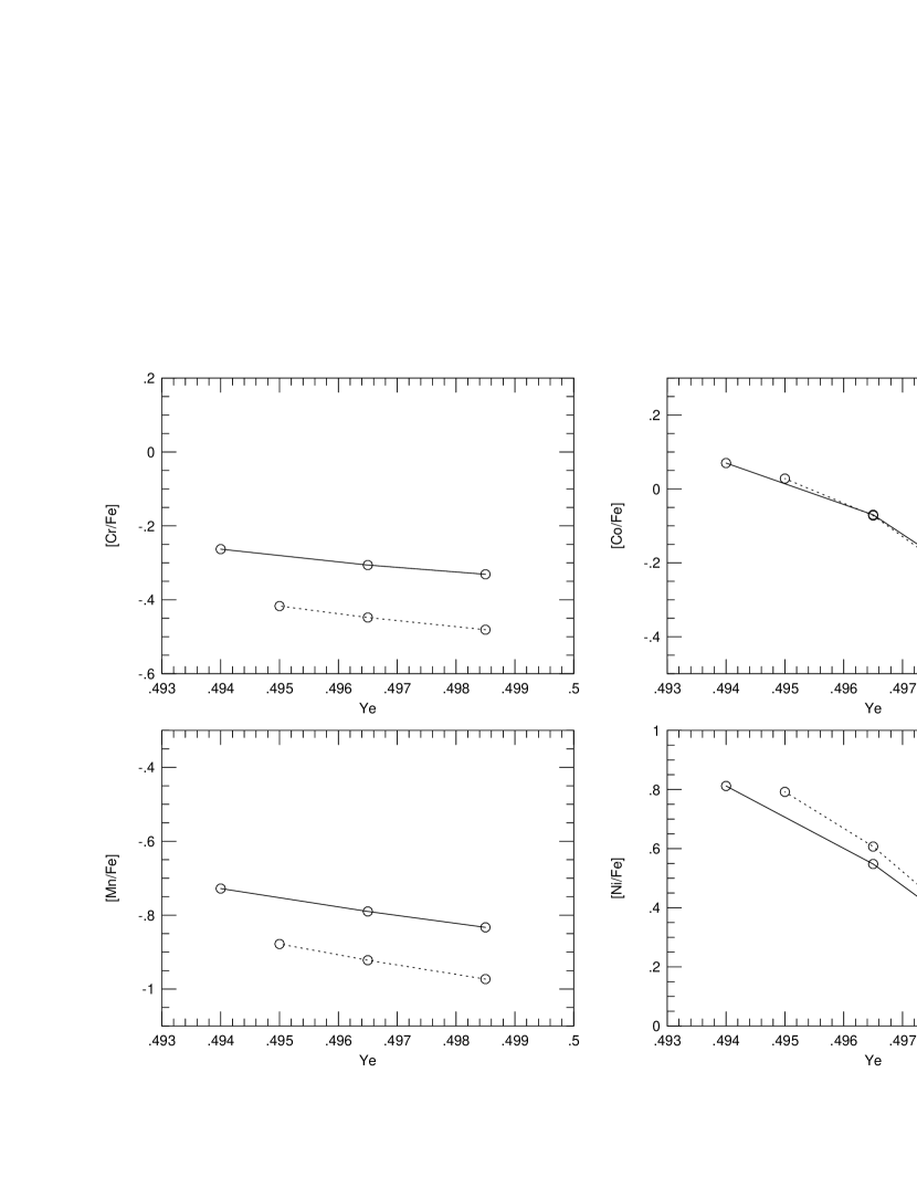
Figure 6.— Dependence on $Y_{e}$. Three models with different $Y_{e}$ are used for each line. Solid line indicates supernovae of $M_{{\rm core}}=6M_{\odot}$, ${\rm E}_{\rm exp}=1.0\times 10^{51}$ergs, $M_{{\rm cut}}=1.418M_{\odot}$. Dotted line indicates $M_{{\rm core}}=8M_{\odot}$, ${\rm E}_{\rm exp}=1.0\times 10^{51}$ergs, $M_{{\rm cut}}=1.419M_{\odot}$.

Figure 7.— Dependence on explosion energy. They have the same progenitor the 8M_⊙ He core and the $Y_{e}^{\rm deep}$ of 0.4985, but the explosion energies are $0.4\times 10^{51}$ergs (left) and $2.0\times 10^{51}$ergs (right).

Figure 8.— Dependence on progenitor mass. Both models have the same explosion energy of $1.0\times 10^{51}$ ergs and a $Y_{e}^{\rm deep}$ of 0.4985, but different progenitors, which are the 6$M_{\odot}$ He core of the 20$M_{\odot}$ star (left) and the 8$M_{\odot}$ He core of the 25$M_{\odot}$ star (right).

Figure 9.— Abundance ratios of various SNe II. Mass cuts of the models are also shown below abundance ratios. Models A and C (B and D, F and G) have different $Y_{e}^{\rm deep}$ values (See Table 3).

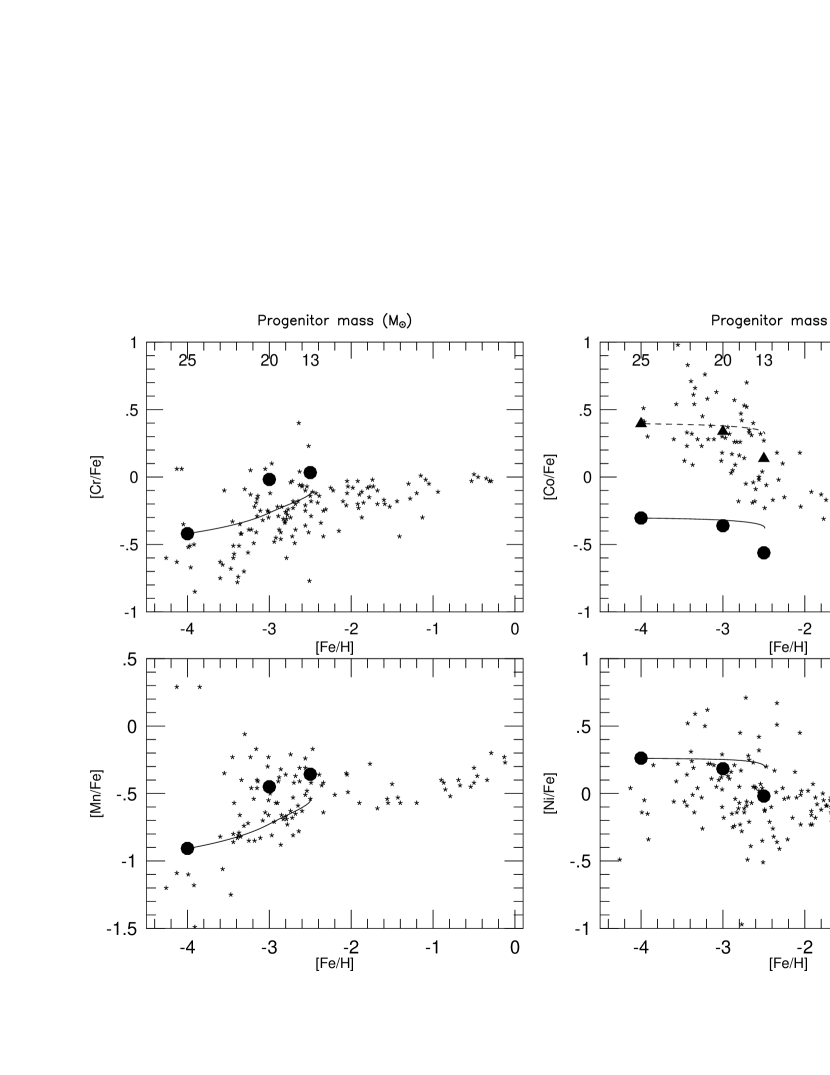
Figure 10.— Variations in the iron-peak abundance ratios. The observational trend between ejected ⁵⁶Ni mass and stellar mass is taken into account. Solid lines and dashed line show ‘well-mixed’ models. ‘Unmixed’ models are also shown in filled circles and filled triangles. The model set [B, G, H] in Figure 9 and Table 3 are used for obtaining these results. The dashed line and the filled triangles indicate the models for which the Co yield is multiplied by five for easier comparison with observed data.

Figure 11.— Same as Figure 10, but with models for making stronger contrast in abundance ratios. The model set [A, G, I] in Figure 9 and Table 3 are used for the solid lines and the filled circles. The dashed line and the filled triangles indicate the models for which the Co yield is multiplied by five for easier comparison with observed data.

Figure 12.— Variations in the iron-peak abundance ratios. The solid lines stand for ‘well-mixed’ models and the filled squares for ‘unmixed’ models. The model set [D, G, H] in Figure 9 and Table 3 are used. The model ’D’ has smaller $Y_{e}^{\rm deep}$ than ‘B’

Figure 13.— Same as Figure 11, but with models for making stronger contrast in abundance ratios. The models [C, F, I] in Figure 9 and Table 3 are used.

Figure 14.— Ejected ⁵⁶Ni mass as a function of main-sequence mass, as estimated for SN II 1987A (Shigeyama & Nomoto 1990); SN IIb 1993J (Shigeyama et al. 1994); SN Ic 1994I (Iwamoto et al. 1994); SN II 1997D (Turatto et al. 1998); SN Ic 1997ef (Iwamoto et al. 1998). The ⁵⁶Ni mass of the models in Figure 9 are shown as open circles.

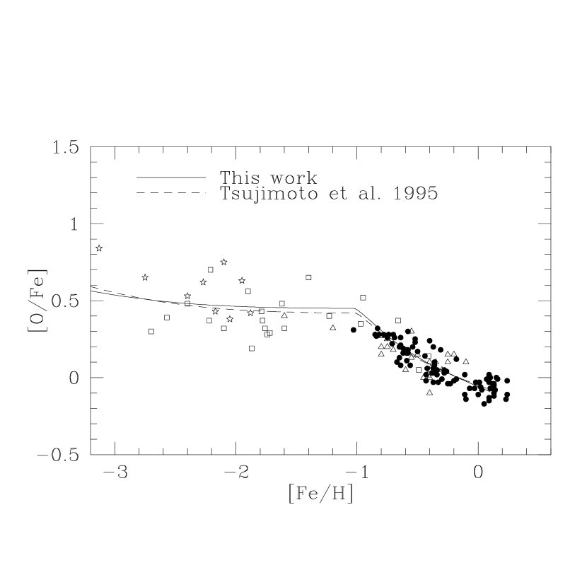
Figure 15.— The evolution of [O/Fe] against [Fe/H] for the different Fe yields from SNe II, i.e., our model with the set [B, G, H] (solid line) and Tsujimoto et al. (1995; dashed line). The observational data are taken from Edvardsson et al. (1993) (filled circles); Barbuy & Erdelyi-Mendes (1989) (open triangles); Nissen et al. (1994) (stars); and Gratton (1991) (open squares).

Table 1Dependence on mass cut.

Model
$M$($M_{\odot}$)	25	25	25	20	20	20
$M_{{\rm core}}$($M_{\odot}$)	8	8	8	6	6	6
E${}_{{\rm exp}}{\footnotesize(\times 10^{51}{\rm ergs})}$	$1.0$	$1.0$	$1.0$	$1.0$	$1.0$	$1.0$
${\bf M_{{\rm cut}}}$($M_{\odot}$)	1.42	1.54	1.62	1.42	1.55	1.62
$Y_{e}^{\rm deep}$	0.4950	0.4950	0.4950	0.4940	0.4940	0.4940
Yield ($M_{\odot}$)							main elem.
Fe	2.44E-01	1.62E-01	1.14E-01	1.72E-01	9.53E-02	5.50E-02	56Ni
Fe	2.44E-01	1.62E-01	1.14E-01	1.72E-01	9.53E-02	5.50E-02	56Ni
Cr	1.30E-03	1.27E-03	1.24E-03	1.31E-03	1.20E-03	1.14E-03	52Fe
Mn	3.38E-04	3.37E-04	3.37E-04	3.35E-04	3.34E-04	3.33E-04	55Co
Co	6.87E-04	4.84E-04	3.01E-04	5.33E-04	2.33E-04	7.00E-05	59Cu
Ni	8.71E-02	5.48E-02	3.64E-02	6.42E-02	2.70E-02	7.16E-03	58Ni
Ratio							solar ratio
Cr/Fe	5.34E-03	7.87E-03	1.09E-02	7.62E-03	1.26E-02	2.08E-02	1.40E-02
[Cr/Fe]	-0.417	-0.249	-0.106	-0.263	-0.044	0.173
Mn/Fe	1.38E-03	2.08E-03	2.96E-03	1.95E-03	3.50E-03	6.05E-03	1.04E-02
[Mn/Fe]	-0.878	-0.700	-0.548	-0.728	-0.475	-0.273
Co/Fe	2.82E-03	2.77E-03	2.64E-03	3.10E-03	1.27E-03	2.45E-03	2.64E-03
[Co/Fe]	0.028	0.022	0.001	0.070	-0.032	-0.316
Ni/Fe	3.57E-01	3.39E-01	3.20E-01	3.74E-01	2.83E-01	1.30E-01	5.76E-02
[Ni/Fe]	0.792	0.770	0.745	0.812	0.692	0.355

Table 2Dependences on $Y_{e}$.

Model
$M$($M_{\odot}$)	25	25	25	20	20	20
$M_{{\rm core}}$($M_{\odot}$)	8	8	8	6	6	6
E${}_{{\rm exp}}{\footnotesize(\times 10^{51}{\rm ergs})}$	$1.0$	$1.0$	$1.0$	$1.0$	$1.0$	$1.0$
$M_{{\rm cut}}$($M_{\odot}$)	1.42	1.42	1.42	1.42	1.42	1.42
$Y_{e}^{\rm deep}$	0.4950	0.4965	0.4985	0.4940	0.4965	0.4985
Yield ($M_{\odot}$)							main elem.
Fe	2.44E-01	2.71E-01	3.05E-01	1.72E-01	1.99E-01	2.21E-01	56Ni
Cr	1.03E-03	1.35E-03	1.41E-03	1.31E-03	1.37E-03	1.44E-03	52Fe
Mn	3.38E-04	3.38E-04	3.39E-04	3.35E-04	3.37E-04	3.38E-04	55Co
Co	6.87E-04	6.05E-04	4.03E-04	5.33E-04	4.47E-04	3.05E-04	59Cu
Ni	8.71E-02	6.31E-02	3.26E-02	6.42E-02	4.05E-02	2.29E-02	58Ni
Ratio							solar ratio
Cr/Fe	5.34E-03	4.97E-03	4.61E-03	7.62E-03	6.89E-03	6.51E-03	1.40E-02
[Cr/Fe]	-0.417	-0.448	-0.481	-0.263	-0.306	-0.331
Mn/Fe	1.38E-03	1.25E-03	1.11E-03	1.95E-03	1.69E-03	1.53E-03	1.04E-02
[Mn/Fe]	-0.878	-0.922	-0.973	-0.728	-0.790	-0.833
Co/Fe	2.82E-03	2.34E-03	1.32E-03	3.10E-03	2.25E-03	1.38E-03	2.64E-03
[Co/Fe]	0.028	-0.072	-0.300	0.070	-0.070	-0.281
Ni/Fe	3.57E-01	2.33E-01	1.07E-01	3.74E-01	2.03E-01	1.04E-01	5.76E-02
[Ni/Fe]	0.792	0.607	0.268	0.812	0.548	0.256

Table 3Type II supernova Models in Figure 9.

Model	A	B	C	D	E	F	G	H	I
$M$($M_{\odot}$)	25	25	25	25	20	20	20	13	13
$M_{{\rm core}}$($M_{\odot}$)	8	8	8	8	6	6	6	3.3	3.3
E${}_{{\rm exp}}{\footnotesize(\times 10^{51}{\rm ergs})}$	$1.0$	$1.0$	$1.0$	$1.0$	$1.0$	$1.0$	$1.0$	$1.0$	$1.0$
$M_{{\rm cut}}$($M_{\odot}$)	1.42	1.47	1.42	1.47	1.42	1.58	1.58	1.32	1.37
$Y_{e}^{\rm deep}$	0.4985	0.4985	0.4950	0.4950	0.4940	0.4940	0.4985	0.4990	0.4990
Yield ($M_{\odot}$)
Fe	3.05E-01	2.62E-01	2.44E-01	2.09E-01	1.72E-01	7.77E-02	9.01E-02	6.87E-02	3.50E-02
Cr	1.41E-03	1.39E-03	1.30E-03	1.29E-03	1.31E-03	1.18E-03	1.21E-03	1.04E-03	9.85E-04
Mn	3.40E-04	3.39E-04	3.38E-04	3.37E-04	3.35E-04	3.33E-04	3.34E-04	3.15E-04	3.14E-04
Co	4.03E-04	3.43E-04	6.85E-04	5.89E-04	5.33E-04	1.63E-04	1.03E-04	4.97E-05	1.09E-05
Ni	3.26E-02	2.75E-02	8.71E-02	7.36E-02	6.42E-02	1.84E-02	7.92E-03	3.79E-03	1.09E-03
56Ni	2.90E-01	2.48E-01	2.25E-01	1.93E-01	1.60E-01	7.04E-02	8.35E-02	6.41E-02	3.17E-02
Ratio
[Cr/Fe]	-0.481	-0.420	-0.418	-0.355	-0.263	0.035	-0.018	0.033	0.305
[Mn/Fe]	-0.973	-0.907	-0.878	-0.812	-0.728	-0.387	-0.450	-0.357	-0.065
[Co/Fe]	-0.300	-0.304	0.027	0.027	0.070	-0.100	-0.361	-0.562	-0.927
[Ni/Fe]	0.268	0.262	0.792	0.785	0.812	0.614	0.184	-0.019	-0.267

References

- Anders et al., (1989) Anders, E., and Grevesse, M. 1989. Geochim. Cosmochim. Acta, 53, 197
- Audouze and Silk (1995) Audouze, J., & Silk, J. 1995, ApJ, 451, L49
- Barbuy et al., (1989) Barbuy, B. & Erdelyi-Mendes, M. 1989, A&A, 214, 239
- Bond et al., (1984) Bond, J. R., Arnett W. D., & Carr B.J. 1984, ApJ, 280, 825
- Burrows (1998) Burrows, A. 1998, in Nuclear Astrophysics, ed. W. Hillebrandt & E. Müller (Gariching: Max Planck Institut für Astrophysik), MPA/P10, 76
- Cioffi et al., (1988) Cioffi, D.F., McKee, C.F. & Bertschinger, E. 1988, ApJ, 334, 252
- Colella et al., (1984) Colella, P., & Woodward, P. R. 1984, J. Comput. Phys. 54, 174
- Edvardsson et al., (1993) Edvardsson, B., Andersen, J., Gustafsson, b., Lamgert, D. L., Nissen, P. E., & Tomkin, J. 1993, A&A, 275, 101
- Gratton (1989) Gratton, R. G. 1989, A&A, 208, 171
- Gratton and Sneden (1987) Gratton, R. G. & Sneden, C. 1987, A&A, 178, 179
- Gratton and Sneden (1988) Gratton, R. G. & Sneden, C. 1988, A&A, 204, 193
- Gratton and Sneden (1991) Gratton, R. G. & Sneden, C. 1991, A&A, 241, 501
- Gratton (1991) Gtatton, R. G. 1991, in IAU symp. 145, Evolution of Stars: The Photometric Abundance Connection, ed. G. Michaud & A. V. Tutukov (Montreal: Univ. Montreal), 27
- Hashimoto et al., (1989) Hashimoto, M., Nomoto, K., & Shigeyama, T. 1989, A&A, 210, 5
- Hix and Thielemann (1996) Hix, W. R. & Thielemann, F.-K. 1996, ApJ, 460, 869
- Iwamoto et al., (1994) Iwamoto, K., Nomoto, K., Höflich, P., Yamaoka, H., Kumagai, S., & Shigeyama, T., 1994, ApJ, 437, L115
- Iwamoto et al., (1997) Iwamoto, K., Young., T. R., Nakasato, N., Shigeyama, T., Nomoto, K., Hachisu, I., & Saio, H., 1997, ApJ, 477, 865
- Iwamoto et al., (1998) Iwamoto, K., Mazzali, P. A., Nomoto, K., Umeda, H., Nakamura, T., Patat, F., Danziger, I. J., Young, T. R., Suzuki, T., Shigeyama, T., Augusteijn, T., Doublier, V., Gonzalez, J.-F., Boe hnhardt, H., Brewer, J., Hainaut, O.R., Lidman, C., Leibundgut, B., Cappellaro, E., Turatto, M., Galama, T. J., Vreeswijk, P. M., Kouveliotou, C., Paradijs, J.van, Pian, E., Palazzi, E., & Frontera F. 1998, Nature, 395, 672
- Kobayashi (1998) Kobayashi, C. 1998, private communication
- Kobayashi et al., (1998) Kobayashi, C. Tsujimoto, T., Nomoto, K., Hachisu, I., & Kato, M. 1998, ApJ, 503, L155
- Magain (1989) Magain, P. 1989, A&A, 209 211
- (22) McWilliam, A., Preston, G.W., Sneden, C., & Shectman, S. 1995a, AJ, 109, 2736
- (23) McWilliam, A., Preston, G.W., Sneden, C., & Searle, L. 1995b, AJ, 109, 2757
- McWilliam (1997) McWilliam, A. 1997, ARA&A, 35, 503
- McWilliam (1998) McWilliam, A. 1998, private communication
- Molaro and Bonifacio (1990) Molaro, P., & Bonifacio, P. 1990, A&A, 236, L5
- Molaro and Castelli (1990) Molaro, P., & Castelli, F. 1990, A&A, 228, 426
- Nakamura et al., (1998) Nakamura, T., Iwamoto, K. & Nomoto, K. 1998, in Origin of Matter and Evolution of Galaxies in the Universe, eds. T. Kajino, & S. Kubono, (Singapore: World Scientific Publishing), in press
- Nissen et al., (1994) Nissen, P. E., Gustaffson, B., Edvardsson, B., & Gilmore, G.. 1994, A&A, 85, 440
- Nomoto et al., (1984) Nomoto, K. Thielemann, F-K., & Yokoi, K. 1984, ApJ, 286, 644
- Nomoto and Hashimoto (1988) Nomoto, K. & Hashimoto, M. 1988, Phys. Rep., 256, 173
- Nomoto et al., (1993) Nomoto, K., Suzuki, T., Shigeyama, T., Kumagai, S., Yamaoka, H., and Saio, H. 1993, Nature, 364, 507
- (33) Nomoto, K., Yamaoka, H., Pols, O. R., Van Den Heuvel, E. P. J., Iwamoto, K., Kumagai, S., & Shigeyama, T. 1994a, Nature, 437, 115
- (34) Nomoto, K., Yamaoka, H., Shigeyama, T., Kumagai, S., & Tsujimoto, T. 1994b, in Supernovae, Les Houches Session LIV, ed. S. A. Bludman et al. (Amsterdam: North-Holland), 199
- Nomoto et al., (1997) Nomoto, K., Blinnikov, S.I., & Iwamoto, K. 1997, in SN1987A: Ten Years After, eds. M. Phillips, & N. Suntzeff (PASP Conference series), in press
- Norris et al., (1993) Norris, J. E., Peterson, R. C., & Beers, T. C. 1993, ApJ, 415, 797
- Osterbrock (1989) Osterbrock, D. E. 1989, “Astrophysics of Gaseous Nebulae and Active Galactic Nuclei”, (Mill Valley: University Science Books)
- Peterson et al., (1990) Peterson, R. C., Kurucz, R. L., & Carney, B. W. 1990, ApJ, 350, 173
- Primas et al., (1994) Primas, F., Molaro, P., & Castelli, F. 1994, A&A, 290, 885
- Ryan et al., (1991) Ryan, S.G., & Norris, J.E. 1991, AJ, 101, 1835
- Ryan et al., (1996) Ryan, S.G., Norris, J.E., & Beers, T.C. 1996, ApJ, 471, 254
- Ryan (1998) Ryan, S.G. 1998, private communication
- Searle and Zinn (1978) Searle, L. & Zinn, T. 1978, ApJ, 225, 357
- (44) Searle, L. & McWilliam, A. 1998, in preparation
- Shigeyama et al., (1987) Shigeyama, T., Nomoto, K., Hashimoto, M., & Sugimoto, D. 1987, Nature, 328, 320
- Shigeyama et al., (1988) Shigeyama, T., Nomoto, K., & Hashimoto, M. 1988, A&A, 196, 141
- Shigeyama et al., (1990) Shigeyama, T., & Nomoto, K., 1990, ApJ, 360, 242.
- Shigeyama et al., (1994) Shigeyama, T., Suzuki, T., Kumagai, S., Nomoto, K., Saio, H., & Yamaoka, H., 1994, ApJ, 420, 341.
- Sollerman et al., (1998) Sollerman, J., Cumming, R. J., and Lundqvist, P. 1998, ApJ, 493, 933
- Thielemann et al., (1990) Thielemann, F.-K., Hashimoto, M., & Nomoto, K. 1990, ApJ, 349, 222
- Thielemann et al., (1996) Thielemann, F.-K., Nomoto, K., & Hashimoto, M. 1996, ApJ, 460, 408
- Timmes et al., (1995) Timmes, F. X., Woosley, S. E., Weaver, T. A. 1995, ApJS, 98, 617
- Tsujimoto et al., (1995) Tsujimoto, T., Nomoto, K., Yoshii, Y., Hashimoto, M., Yanagida, Y., & Thielemann, F.-K. 1995, MNRAS, 277, 945
- Tsujimoto et al., (1997) Tsujimoto, T., Yoshii, Y., Nomoto, K., Matteucci, F., Thielemann, F.-K. & Hashimoto, M. 1997, ApJ, 483, 228
- Turatto et al., (1998) Turatto, M., Mazzali, P. A., Young, T. R., Nomoto, K., Iwamoto, K., Benetti, S., Cappellaro, E., Danziger, I. J., de Mello, D. F., Phillips, M. M., Suntzeff, N. B., Clocchiatti, A., Piemonte, A., Leibundgut, B., Covarrubias, R., Maza, J., Sollerman, J., 1998, ApJ, 498, L129
- Woosley et al. (1973) Woosley, S.E., Arnett, W. D., Clayton, D. D. 1973, ApJS, 26, 231
- Woosley et al., (1988) Woosley, S.E., Pinto, P.A., & Ensman, L. 1988, ApJ, 324, 466
- Woosley et al., (1995) Woosley, S.E., & Weaver, T.A. 1995, ApJS, 101, 181
- Zhao and Magain (1990) Zhao, G. & Magain, P. 1990, A&A, 238, 242