High spectral and time resolution observations of the eclipsing polar RX J0719.2+6557

Abstract

We present phase-resolved spectral and multicolor CCD-photometric observations of the eclipsing polar RX J0719.2+6557 obtained with relatively high time ($\approx$600 sec/15 sec) and spectral (2.1 Å) resolution when the system was in a high accretion state. The trailed spectrograms clearly reveal the presence of three different line components with different width and radial velocity variation. The Balmer emission lines, as well as the higher excitation He ii line, contain significant contributions from the X/UV-illuminated hemisphere of the companion star. We were able to resolve all three components by line deblending, and by means of Doppler tomography were able to unambiguously identify the emission components with the secondary star, the ballistic part of the accretion stream and the magnetically funnelled part of the stream. The light curves and eclipse profiles provide additional information about the system geometry.

¹OAN, Instituto de Astronomía,UNAM, México
²Department of Astronomy, University of Washington, Seattle, USA
³Astrophysical Institute Potsdam, Potsdam, Germany
⁴Dept. of Astronomy, University of Cape Town, South Africa
⁵Sternwarte Sonneberg, 96515 Sonneberg, Germany
⁶University of Wyoming, Laramie, Wyoming, USA
⁷Department of Astronomy, NMSU, Las Cruces, New Mexico, USA

1. Introduction

The X-ray source RX J0719.2+6557  was discovered during the ROSAT All Sky Survey and identified as an eclipsing polar by Tovmassian et al. (1997)(T97). The authors found that the system undergoes deep eclipses (3 mag), with flat light curve out of eclipse in the blue and with pronounced sinusoidal variations in red light. The orbital period estimated at $P_{\rm orb}=0.068207$ day based on the eclipse occurrence, coincided with radial velocity variations obtained from the spectroscopy. T97 showed that the line profiles are multi-component and were able to identify two components with difficulty.

Here we report on new observations of RX J0719.2+6557  with improved spectral and time characteristics that allow us to conduct a detailed study of the various components of this eclipsing polar.

2. Data acquisition and reduction

We obtained spectra of RX J0719.2+6557  during two half nights with the 3.5m ARC telescope at Apache Point Observatory using the DIS spectrograph set in two wavelength regions $4200-5100\rm\AA$ and $7900-8900\rm\AA$ with spectral resolution of $1.3\rm{\AA/pix}$, corresponding to overall FWHM resolution $2.4\rm\AA$. We also acquired fast photometry at APO using SpiCam in three broad band filters (B V R), covering one orbit in each band. We observed the object in the IR J H K filters simultaneously with the spectroscopy during poor weather conditions in Wyoming. We also collected more unfiltered (red) light CCD-photometry from Sonneberg and Red Buttes Observatory (RBO).

3. Analysis and results

3.1. Orbital period and eclipse phase

Based on the new photometric data combined with eclipse moments reported in (T97) we refined the orbital period of RX J0719.2+6557. We should note here that this ephemeris refers to the eclipse phasing or photometric phase. Later we will show that the spectral phase differs from the photometric phase.

3.2. Irradiated secondary

We used the optical photometric data obtained without filter at RBO with CCD sensitive in the far red (corresponding to R+I) along with B&R light curves obtained at the 3.5m ARC telescope for a study of periodic variations outside the eclipse. After eliminating the eclipse points, we fitted the light curves with a simple sine function. In the case of the red unfiltered light curve we just dismissed the points corresponding to the eclipse. For the ARC data we normalized the depth of eclipse in B to the one in R and subtracted the former from latter. The red light curve obtained at RBO and the fitted curve are shown in Fig. 1. The minima in the R band occur at $\delta\phi_{\rm orb}=0.06$ prior to the eclipse. An identical result was obtained for the APO data. The modulation is single humped relative to the orbital period. We presume that this modulation in red light is due to the irradiated side of the secondary component. The phase lag between the minimum of the single humped curve and the eclipse has two possible explanations, which might both contribute to the large amount of the observed lag. One explanation is that the occulting source is not the white dwarf, but the bright spot on the accretion stream in the coupling region. Another possible cause of the phase lag is uneven irradiation of the leading side of the secondary due to its obscuration by a stream leaving the L1 point.

Figure 1.: Left: R light curve and fit by a $sin$ curve (out of eclipse, top) and the spectroscopic coverage (bottom). The eclipse and the minima of the $sin$ curve

are shown by vertical lines. Right: BVR light curves at different scales.

3.3. Eclipse light curves

Fig. 1 (right panel) shows three eclipse light curves in different broad band filter B, V & R. They are presented on three panels with different scales to distinguish details at different orbital phases. On the lower panel one can see that the eclipse actually consists of two parts. The first section is relatively broad and shallow, while the second is narrower and deeper. The $\approx 4$ mag depth of eclipse in B is evidence that the compact structure that is occulted is a major source of light. The errors at the bottom of eclipse are too big to be able to make more precise estimates. The various steps of eclipse are marked by vertical lines in the figure. The total eclipse lasts about 505 sec. Meanwhile the deep eclipse duration at half depth is $245\pm 20$ sec, which corresponds to half width at half depth $\phi_{1/2}=7\hbox{$.\!\!^{\circ}$}5\pm 2\hbox{$.\!\!^{\circ}$}0$ as defined by Bailey (1990).

The eclipse profile is similar to that of 1H 1752+081 possibly containing an accretion disk (Silber et al. 1994), although there are contradictions in photometry and spectroscopy with that explanation. At the same time, Barwig et al. (1994) interpret this eclipse profile as an eclipse of the white dwarf followed immediately by the accretion stream, i.e. the white dwarf is being eclipsed first (step 1), then the accretion stream (step 2). Step 3 corresponds to the egress of white dwarf and finally egresses the stream (step 4). It makes sense in the case of 1H 1752+081 where the depth of both eclipse phases (1 & 2) are about the same, and one can pair 1st with 3rd (2nd with 4th) on the basis of their steepness. However, in case of RX J0719.2+6557  this scenario is not applicable, since the initial occultation (step 1) is very shallow as well as the final egress (step 4) in comparison to the central dip. One remote possibility would be to suppose that the first step corresponds to the ingress of unspotted part of the white dwarf, while the second phase is the mixed ingress of spot on the second half of the white dwarf and stream, with white dwarf egress resulting in step 3 and finally stream (step 4). To test this scenario higher accuracy and faster photometry at the bottom of the eclipse would be needed to prove if it is either flat as it seems in the B light curve or structured as it looks in V and R data. Until then, taking into account the above mentioned phase lag between eclipse and minimum in red light and possible variability of the eclipse profile, we tend to think that a more plausible cause of the eclipse is the occultation of the stream with the bright spot elevated some distance over the white dwarf surface.

3.4. Spectroscopy

We used the three brightest lines in our spectral range H$\beta$, H$\gamma$ and He ii for our analysis. The line profiles are very complex. They look similar, but the Balmer lines are more blury than He ii and the components seem less resolved. Hence, in order to study the components of the emission lines, we started with the He ii line. We stacked the spectra into a bidimensional image to construct trailed spectra (Fig. 2). They were placed in order of orbital phases (calculated according the photometric ephemeris). Each line corresponds to approximately 0.05 orbital phase. In the trailed spectra the so called narrow component is easily distinguished. It is more pronounced at phases 0.15–0.85 being the brightest feature there. The other noticable feature is a high velocity component (HVC) which is shaping the edges of the emission line around phases 0.0 and 0.5.

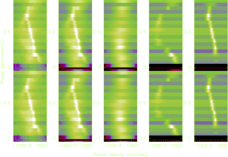
Figure 2.: Trailed He ii spectra of RX J0719.2+6557: as observed (left), the computed composite of three gaussians (second from left) and the three gaussians separately.

The common procedures for line measurements, such as gaussian deconvolution for example, do not work in this case. Thus, we measured the above mentioned component centers “manually” on the zoomed trailed spectra image. These gave us enough points to fit sine curves to both of them with the photometric period and to estimate the central wavelenghts of both components at each phase. We used these interpolated line centers in the line deblending procedure available in IRAF to define the central wavelengths of the components more precisely. We did another iteration supplying the fitted values to the deblending procedure and found that two components can not account for the entire line profile. We subtracted both components from the actual line profile and measured the center of the remaining broad component. It also displayed wavelike variation appropriate to the orbital period of the system. We did yet another iteration by supplying the deblending procedure with three components before we were satisfied with the results. At eclipse and phases immediately after or before, we failed to identify all three components, and at some phases it was difficult to distinguish between them. Nevertheless the resulting profiles and corresponding radial velocity curves are quite reasonable (Fig. 3). The radial velocity curves of three components are also presented in Fig. 3 (right panel). Among other interesting features to be seen in the radial velocity phasing, the most striking is the time lag between the zero velocity crossing of secondary (conjunction) and eclipse, which happens $\delta\phi=0.06$ phase later. That coincides exactly with the result drawn from photometry. The similar results were obtained from hydrogen lines analysis.

Figure 3.: Left: Profiles of the He ii line and deblending components (dashed lines). The solid line is the sum of all three components. Right: The radial velocities of the three components and $sin$ fits.

4. Some constraints

Figure 4.: Accretor mass versus mass ratio. Dashed lines mark inclinations of $i$=90^∘, 80^∘ and 70^∘ (from bottom to top) with the two values of K2=400 and 450 km/s each. Two M₁ values are marked for different secondary masses depending on their spectral class (dotted lines) and the condition for a Roche lobe filling secondary is drawn as solid line.

In summary, we have the following observational data for consideration of the system parameters: (i) the orbital period $P_{orb}=5893.13$ sec, (ii) the radial velocity amplitude ${K_{2}}^{{}^{\prime}}$=323 km/sec for He ii and 379 km/sec for composite $H\beta$/$H\gamma$ data (iii) the eclipse half width at half depth $\phi_{1/2}=7\hbox{$.\!\!^{\circ}$}5\pm 2\hbox{$.\!\!^{\circ}$}0$ (as defined by Bailey 1990) and (iv) $i$ $\mathrel{\hbox{\raise 2.15277pt\hbox{$>$}\hbox to0.0pt{\hss\lower 2.15277pt\hbox{$\sim$}}}}$75^∘ due to eclipses. Now, if we make a number of assumptions, we can estimate different parameters of the system. The basic assumptions common for most CVs are that the secondary is a pre-main sequence star filling its Roche lobe and obeying the mass-radius relation for main-sequence stars. Assuming in addition that the RV of the narrow line component reflects the motion of the irradiated secondary, then after applying a reasonable correction for the center of mass of the secondary, we get a range of 400 to 450 km/sec. Taking into account the inclination, period and velocity amplitude we can constrain the mass of the primary WD. The resulting diagram of the $M_{1}$ dependence from $\rm{q=M_{2}/M_{1}}$ is plotted in Fig. 4. Combining the relation between the binary component masses and the Roche lobe size as suggested by Iben & Tutukov (1984), with the mass-radius relation of low-mass main-sequence stars we calculate the condition for a Roche lobe filling secondary. The resulting q range of 0.15–0.3 is in agreement with the expected M 4–5.5 spectral type for the secondary according to the orbital period to spectral type relation.

We can further constrain the inclination and mass ratio by using the observed eclipse width if we assume that the occulted source is the white dwarf. If the companion in RX J0719.2+6557  fills its Roche lobe, the eclipse half width at half depth of about 7$.\!\!^{\circ}$5 defines a unique relation between the mass ratio q and the inclination of the system with respect to the line of sight (Chanan et al. 1976). This relation crosses the line of the Roche lobe filling condition at i=79$\pm$3^∘. If the secondary is an unevolved main-sequence star just filling its Roche lobe, then this inclination implies the following solution: a white dwarf mass of $\rm{M_{1}=0.75}\pm 0.1$M_⊙  and a companion mass of $\rm{M_{2}=0.13}\pm 0.05$M_⊙  (q=0.175). In the case of an M5 companion (implying an evolved state to allow Roche lobe filling) $\rm{M_{1}=0.85}\pm 0.1$M_⊙  and $\rm{M_{2}=0.21}\pm 0.05$M_⊙  (q=0.25) is also a viable solution.

References

Chanan, G.A., Middleditch, J., Nelson, J.E., 1976, ApJ, 208, 512

Bailey, J., 1990, MNRAS, 243, 57

Barwig, H., Ritter, H., Barnbanter, O., 1994 , A&A, 288, 204

Iben, I., Tutukov, A.V., 1984, ApJ, 284, 719

Silber, A.D., Remillard, R.A., Horne, K., Bradt, H., 1994, ApJ, 424, 955

Tovmassian, G.H., Greiner, J., Zickgraf, F.-J., Kroll, P., Krautter, J., Thiering, I., Zharykov, S.V., Serrano, A., 1997 (T97), A&A, 328, 571