Spectroscopy of the roAp star $\mn@boldsymbol{\alpha}$ Cir – II.
The bisector and equivalent-width of the H$\mn@boldsymbol{\alpha}$ line

Abstract

We present bisector measurements of the H$\alpha$ line of the rapidly oscillating Ap (roAp) star, $\alpha$ Cir, obtained from dual-site observations with medium-dispersion spectrographs. The velocity amplitude and phase of the principal pulsation mode vary significantly, depending on the height in the H$\alpha$ line, including a phase reversal between the core and the wings of the line. This supports the theory, suggested in Paper I, of a radial pulsational node in the atmosphere of the star. Blending with metal lines partially affects the H$\alpha$ bisector results but probably not enough to explain the phase reversal.

We have also detected changes in the equivalent-width of the line during the pulsation, and measured the oscillatory signal as a function of wavelength across the H$\alpha$ region.

1 Introduction

Rapidly oscillating Ap (roAp) stars are a sub-class of chemically peculiar magnetic (Ap or CP2) stars. They pulsate with photometric amplitudes below 8 mmag and periods in the range 5–15 minutes. $\alpha$ Cir (HR 5463, HD 128898) is the brightest of the known roAp stars ($V=3.19$). Previous observations of this star in photometry have shown that it has one dominant pulsation mode with a period of 6.825 min ($f=2442$ $\mu$Hz; Kurtz et al. 1994, hereafter KSMT). Medupe & Kurtz (1998) observed that the amplitude decreased with increasing wavelength, from $2.71\pm 0.18$ mmag  in Johnson $U$ (3670Å) to $0.41\pm 0.13$ mmag in $I$ (7970Å). They proposed that the rapid decline of photometric amplitude with wavelength could be explained by a decrease in the temperature amplitude of the pulsation with atmospheric height.

Baldry et al. (1998a, hereafter Paper I) showed that the velocity amplitude and phase of the principal pulsation mode in $\alpha$ Cir  varied significantly from line to line. However, it was difficult to interpret the data because of blending effects. In particular, there was evidence for a velocity node in the atmosphere of $\alpha$ Cir but it was uncertain whether the node was horizontal or radial. In this paper we look at the H$\alpha$  line in more detail using the same set of observations, taken during two weeks in 1996 May. These observations comprise 6366 intermediate-resolution spectra taken using the 74 inch (1.88-m) Telescope at Mt. Stromlo, Australia and the Danish 1.54-m Telescope at La Silla, Chile (see Section 2 from Paper I for further details).

We first examined how the H$\alpha$  profile changed during the principal pulsation cycle, in terms of the bisector at different heights in the line (preliminary results were presented by Baldry et al. 1998b). In this way, the effect of the velocity on the profile could be analysed. To quantify the temperature effect, we measured the equivalent-width (EW) amplitude of the principal mode in filters of varying width and measured pixel-by-pixel intensity changes across the H$\alpha$  region of the spectrum. Finally, we defined an observable quantity (related to the EW of H$\alpha$) which had a high signal-to-noise ratio for the principal pulsation. Using this observable, some of the weaker modes in $\alpha$ Cir  were detected.

1.1 General Properties of $\alpha$ Cir

Before we discuss the pulsation of $\alpha$ Cir, we will review the general properties in the light of a recent spectral analysis (Kupka et al. 1996) and the Hipparcos parallax measurement (ESA 1997). The distance of $16.4\pm 0.2$ pc (parallax of $61.0\pm 0.6$ mas), combined with a bolometric correction of $-0.12\pm 0.02$ ($M_{\rm bol,\sun}=4.64$, Schmidt-Kaler 1982), gives $M_{\rm bol}=2.00\pm 0.04$ ($L=11.4\pm 0.4L_{\sun}$). From this luminosity and the temperature of $T_{\rm eff}=7900\pm 200$ K (derived by Kupka et al.), we obtain $R=1.81\pm 0.11R_{\sun}$ (angular diameter of $1.03\pm 0.07$ mas). Combining this radius with $\log g=4.2\pm 0.15$ (Kupka et al.) gives a mass of $M=1.9\pm 0.6M_{\sun}$. The rotation period of 4.48 days (derived by KSMT) and the radius means that $v_{\rm rot}=20.4\pm 1.2$ kms^-1. Using $v\sin i=13\pm 1$ kms^-1(Kupka et al.), the inclination of the rotation axis to the line of sight is then $i=40\degr\pm 5\degr$. This is an improvement on the estimate given by KSMT due to more recent results.

1.2 The Oblique Pulsator Model

In some roAp stars, including $\alpha$ Cir, the amplitude of the oscillations has been observed to be modulated by the rotation period of the star. In particular, the amplitude is at a maximum when the observed magnetic field strength is also at a maximum. This led to the oblique pulsator model (Kurtz 1982), in which an roAp star pulsates non-radially with its pulsation axis aligned with the magnetic axis. The amplitude modulation comes from the inclination of the pulsation axis with respect to the rotation axis. Therefore different aspects of a non-radial mode are viewed as the star rotates. The oblique pulsator model predicts that, in the Fourier domain, a frequency of mode $\ell$ is split into 2$\ell$ +1 frequencies. The frequency splitting is exactly equal to the rotation frequency, and the relative amplitudes are determined by both the inclination of the rotation axis to our line of sight ($i$) and the angle between the rotation axis and the pulsation axis ($\beta$). Most of the review papers mentioned in the Paper I discuss the oblique pulsator model, a refinement of which is given by Shibahashi & Takata (1993).

The principal pulsation mode in $\alpha$ Cir is believed to be a pure oblique dipole mode ($\ell=1$). KSMT observed a 21 percent full-range variation of the amplitude during the rotation period. This variation implies that $\tan i\tan\beta=0.21\pm 0.01$ (see Section 4.1 from KSMT). Using our new estimate of $i$ (see Section 1.1), we get $\beta=14\degr\pm 3\degr$. This means that the inclination angle of the pulsation axis to the line of sight ($\alpha$) varies between 26°  and 54°  during the rotation cycle.

2 General Data Reductions

Extraction of spectra and continuum fitting were done using IRAF procedures (see Section 3.1 from Paper I). We made a number of types of measurements on the reduced spectra, including bisector line-shift measurements which are described in Section 2.2. The time series analysis of these is explained in Section 2.3 and is also applicable to other measurements, which are described later in the paper. Since the continuum fit is more critical than for Paper I, we first describe this procedure in more detail.

2.1 Continuum Fitting

The IRAF procedure continuum was applied to each spectrum in our data, using the following parameters: sample=@list, naverage=1, function=legendre, order=3/4 ‘meaning 2nd/3rd order polynomial’, low_rej=2, high_rej=4, niterate=20/25, grow=0.

Initially, a sample of about 1400 points from each spectrum was used to make a least-squares polynomial fit — 3rd order for the Stromlo data and 2nd order for the La Silla data. A higher order fit was used for the Stromlo data because the continuum shape was less stable. Next, points below 2$\sigma$ and above 4$\sigma$ from the fit were excluded from the next fit. The lower cutoff was used to exclude some absorption lines and the upper cutoff only excluded cosmic ray events. The fitting and excluding routine was repeated 20 to 25 times or in most cases until no more points were excluded. In the final fit, about 1000 points were included, with none being within 50Å of the core of the H$\alpha$  line. Not all absorption lines were excluded from the final fit since there is very little real continuum at the resolution of our data ($\sim$1.5Å). The real continuum level in each fitted spectrum was around 1.005–1.010, depending on the wavelength. Therefore, we have scaled the spectra so that the continuum level is $\sim$1.00 in the H$\alpha$  region of the spectrum. The level varied slightly from spectrum to spectrum, with a standard deviation of about 0.001.

2.2 Bisector Measurements of H$\alpha$

Figure 1: The H$\alpha$  line in $\alpha$ Cir. The dotted lines divide the 22 contiguous sections.

Table 1: Amplitudes and phases of the principal pulsation mode for the bisector velocity at different heights in the H$\alpha$ line. The line was divided into 22 non-overlapping and two extra horizontal sections. For the results in this table, the Stromlo and the La Silla data sets were combined.

section	low	high	mean	velocity	velocity	S/N	velocity	phase
no.	cutoffa	cutoffa	widthb	ampl.c	noised		phasee	errorf
			(Å)	( ms-1)	( ms-1)		(°)	(°)
0	0.39	0.41	1.1	264	19	14.1	333	4
1	0.41	0.43	1.4	256	15	17.4	328	3
2	0.43	0.45	1.7	279	15	18.8	327	3
3	0.45	0.47	1.9	277	15	18.7	327	3
4	0.47	0.49	2.2	257	15	16.9	328	3
5	0.49	0.51	2.5	227	15	14.7	330	4
6	0.51	0.53	2.7	193	16	11.9	333	5
7	0.53	0.55	3.0	176	18	9.6	331	6
8	0.55	0.57	3.5	125	18	6.9	331	8
9	0.57	0.59	3.9	43	18	2.4	303	24
10	0.59	0.61	4.6	54	20	2.8	255	21
11	0.61	0.63	5.4	55	21	2.6	283	22
12	0.63	0.65	6.2	43	23	1.9	334	32
13	0.65	0.67	7.1	26	25	1.0	304	73
14	0.67	0.69	8.3	64	29	2.2	205	27
15	0.69	0.71	9.7	25	33	0.8	—	—
16	0.71	0.73	11.6	254	37	6.8	195	8
17	0.73	0.75	13.0	340	34	10.1	192	6
18	0.75	0.77	14.4	310	36	8.5	191	7
19	0.77	0.80	19.0	181	45	4.0	215	14
20	0.80	0.85	23.9	514	44	11.7	45	5
21	0.85	0.91	32.2	208	56	3.7	18	16
22	0.70	0.72	10.5	86	36	2.4	200	25
23	0.76	0.78	15.3	221	45	4.9	195	12

^aBoundary of the section in relative intensity.
^bApproximate mean width of the line at the height of the section.
^cAmplitude measured at 2442.03 $\mu$Hz.
^drms-noise estimated from amplitude spectrum using the regions 1100–2300 $\mu$Hz and 2600–4400 $\mu$Hz.
^ePhase measured at 2442.03 $\mu$Hz, with respect to a reference-point ($t_{0}$) at JD 2450215.07527, with the convention that a phase of 0° represents maximum of the observed variable.
^fError in the phase is taken to be arcsin (rms-noise/amplitude).

The H$\alpha$  line in each spectrum was divided into 22 contiguous horizontal sections (see Fig. 1 and Cols. 1–4 of Table 1) and two extra sections for checking. For each section, the average wavelength of each side of the absorption line was measured, and a bisector line-shift (average position of the two sides) was calculated. We have used a telluric O₂ band as a Doppler shift reference (see Section 3.3 from Paper I for details).

An alternative method was also tried in which a least-squares fit was made to the position of each side of the line. A template spectrum was used to define the shape of the line and was shifted from side to side until a best fit was obtained. This method produced similar results and noise levels to the method of calculating the average wavelength, but the computational time was longer.

2.3 Time Series Analysis

For each section of the H$\alpha$  line, the above analysis produced a time series of 6366 bisector line-shift measurements (4900 from Stromlo, 1466 from La Silla). Each time series was high-pass filtered and then cleaned for bad data points by removing any points lying outside $\pm 6.5$ times the median deviation. Typically, about 100 data points were removed. Next, a weighted least-squares sine-wave fitting routine was applied (using heliocentric time) to produce amplitude spectra.

For the analysis of the principal pulsation mode in $\alpha$ Cir, we have measured the amplitude and phase of each time series at 2442.03 $\mu$Hz  and estimated the rms-noise level by averaging over surrounding frequencies, 1100–2300 $\mu$Hz  and 2600–4400 $\mu$Hz. The phases are measured at a temporal phase reference point ($t_{0}$) with the convention that a phase of 0° represents maximum of the observable. $t_{0}$ was chosen to coincide with maximum light using data supplied by Don Kurtz (private communication); see Paper I for details. For the phase error, we have used simple complex arithmetic to find the maximum change in phase that an rms-noise vector could induce, i.e., arcsin (rms-noise/amplitude).

3 Bisector Velocities

3.1 Results

Figure 2: Amplitudes and phases of the principal pulsation mode for the bisector velocity at different heights in the H$\alpha$  line. Points with solid lines represent the Stromlo data and points with dotted lines represent the La Silla data. For each measurement, the vertical line is an error-bar while the horizontal line shows the extent of the section in the H$\alpha$  line.

Figure 3: The H$\alpha$  line in $\alpha$ Cir. The crosses show the mean position of the bisector. The wavelength is measured with respect to the centre of the line. The dotted line shows the shape of trapezium filter no. 2, which is used for the equivalent-width measurements. It is plotted using a different vertical scale.

We have assumed that the bisector line-shift measurements represent velocities in the star. The velocity amplitudes and phases of the principal mode at different heights in the H$\alpha$  line are shown in Fig. 2 and Table 1. The results describe the oscillations in the bisector about the mean position at each height (see Fig. 3 for the bisector shape). From 0.4 to 0.8 in the line, the amplitude decreases from 300 ms^-1  to zero and then increases again, with a change in phase of $-$140°. Note that there is good agreement between the Stromlo and La Silla data sets, which were analysed separately for Fig. 2. This gives us confidence that the observed variations are intrinsic to the star.

In Paper I, the H$\alpha$  velocity amplitude and phase were measured to be $\sim$170 ms^-1  and $\sim$330°  using a cross-correlation method. This is compatible with our bisector velocity results since the cross-correlation measurement would be dominated by the steepest part of the H$\alpha$  profile, near the core.

To further illustrate the behaviour of the H$\alpha$  bisector, in Fig. 4 we show the bisector velocity as a function of time and height. The horizontal axis covers two cycles of the principal pulsation mode ($P=6.825$ min). Only sections 0–19 are shown (see Table 1), since above a height of 0.8 the measurements are significantly affected by line blends (see Section 3.2). The figure clearly illustrates that the higher sections are pulsating nearly in anti-phase with the lower sections, and that the velocities of the middle sections are close to zero. Since the bisector velocity reflects the velocity at different heights in the atmosphere, these results support the hypothesis, suggested in Paper I, of a radial node in the atmosphere of $\alpha$ Cir.

Figure 4: Velocity field diagram. The arrows represent bisector velocity vectors, relative to the mean velocity of the star, at different times throughout two pulsation cycles of the principal mode ($P=6.825$ min). The velocity vectors are calculated from the amplitudes and phases of sections 0–19 given in Table 1.

3.2 Blending Considerations

We attribute the velocity node (at $\sim$0.65) and the phase jump between 0.4 and 0.8 to H$\alpha$  line-formation effects, although there is some uncertainty as to how much blending affects the results between heights 0.7 and 0.8. Above a height of 0.8, the results are significantly affected by line blending. In order to identify any metal lines in the wings of H$\alpha$, we used a synthetic spectrum calculated by Friedrich Kupka (private communication) and high-resolution spectra of $\alpha$ Cir taken in 1997 March (coudé echelle, 74 inch Telescope, Mt. Stromlo). From this, we determined that most of the lines blended with the H$\alpha$ profile from 6540Å to 6585Å are telluric, including all those below a height of 0.7 in the H$\alpha$ line.

At height 0.82, the anomalously large velocity amplitude is probably caused by the metal absorption line Sr I 6550.2Å, with the possibility that Fe I 6575.0Å also contributes. Since metal lines can have amplitudes as large as 1000 ms^-1  (Paper I), this can explain the large bisector velocity seen at this height. At height 0.88, the amplitude is similar to that between 0.72 and 0.79 but the phase is anomalous. This measurement is affected by various metal and telluric lines, in particular a metal line blend including Mg II 6546.0Å and Fe I 6546.2Å.

Below a height of 0.8, we expect any absorption features to have less impact on the bisector velocity due to the increasing steepness of the H$\alpha$  profile. However, there is a metal line Fe I 6569.2Å in addition to a few telluric lines that affect the H$\alpha$ profile between 0.7 and 0.8. This Fe I feature affects the bisector measurements between 0.71 and 0.76. Therefore, it probably causes the jump in amplitude near height 0.72 shown in Fig. 2. It cannot explain why all the bisector velocities from heights 0.67–0.80 have phases around 190°–200°, but it does lower the significance of the phase jump between the core and this part of the wings. We speculate that without this Fe I feature, the H$\alpha$ bisector velocity amplitude would increase steadily from 0.70 to 0.77.

In summary, we believe features in Fig. 2 below height 0.7 reflect genuine effects in the H$\alpha$  profile, while those above 0.8 are dominated by metal and telluric lines. Between 0.7 and 0.8, a blend probably exaggerates the phase reversal by causing an increase in the measured amplitude around height 0.73.

3.3 Simulations

Two sources of noise for the velocity measurements, especially at high levels in the H$\alpha$  line, are errors in the continuum fit and changes in the total equivalent-width (EW) of the line (which are expected due to temperature changes during the pulsation cycle). These sources will affect the bisector velocity if the line is asymmetrical at that height. To investigate, we first simulated fluctuations in the EW of the line and measured the resulting pseudo-velocity amplitude, and then simulated fluctuations in the continuum level. We concluded that, while there could be systematic changes in the velocity amplitude greater than 150 ms^-1  above a height of 0.65, the phase of the systematic change would be opposite between height 0.72 and 0.76. This means that this effect cannot explain the different phase of heights 0.72–0.79 compared to heights 0.40–0.56. Perhaps, this systematic effect could explain the large difference in velocity amplitude between height 0.70 and 0.72.

We also considered the effect of a systematic change in the slope of the continuum across the H$\alpha$  line. This could arise because the continuum fit is not entirely independent of the metal lines and, since there are significantly more metal lines on the blueward side of H$\alpha$, the slope of the continuum may vary during the pulsation cycle. We have simulated the effect on the velocity amplitude of a continuum variation having a slope change of 0.001 / 100Å. We found that such a large slope change could produce a systematic change in the velocity amplitude greater than 300 ms^-1  above a height of 0.75 and thus mimic a velocity phase reversal. However, the simulation fails to reproduce a velocity node at 0.65 and other features of Fig. 2. Furthermore, from calculations of the intensity variations in various regions of the spectrum, we do not expect any systematic continuum slope changes to be larger than 0.0001 / 100Å.

Our simulations show that continuum level, continuum slope and H$\alpha$ EW changes cannot account for the observed features of Fig. 2. Therefore, we conclude that the node and phase reversal are caused by the velocity field of the star. Note that random variations in the continuum level and slope may be larger than tested for, but this will only effect the noise level in the amplitude spectra.

3.4 Discussion

Hatzes (1996) has simulated line-bisector variations for non-radial pulsations in slowly rotating stars. His simulations show that a bisector velocity phase reversal could occur in modes with $\ell=m\geq 3$ (see Fig. 3 from Hatzes 1996). In fact, the H$\alpha$  line-bisector variations in $\alpha$ Cir could closely be described by his simulations with $\ell=m=3$ or 4. However, he does not take into account any changes in pulsational amplitude with depth and the simulations were done for much narrower metal lines. Given that there is strong evidence for the $\ell=1$ oblique pulsation model (KSMT), we suggest that a change in pulsational amplitude with depth is a more likely explanation for the bisector variations.

It is interesting to note that similar behaviour to that seen in $\alpha$ Cir has been seen in the Sun. Deubner, Waldschik & Steffens (1996) have observed a phase discontinuity in the solar 3-min oscillations using spectroscopy. In particular, they measured phase differences between the velocity of the core of the NaD₂ line and various positions in the wing (called V$-$V phase spectra). They discovered a 180°  phase jump in the V$-$V spectra near a frequency of 7000 $\mu$Hz. They also observed a phase discontinuity in the V$-$I (Line Intensity) spectra at a similar frequency.

The 3-min oscillations are thought to be formed in an atmospheric (or chromospheric) cavity. Deubner et al. (1996) suggested a model to explain the phase discontinuities, involving running acoustic waves and atmospheric oscillation modes, one of which must have a velocity node in the observed range of heights in the atmosphere.

In the solar model, the eigenfunction of a p-mode with $\ell=1$ and $n=25$ has a radial node separation in the outer part of the Sun of $\sim$0.3 percent of the radius (Christensen-Dalsgaard 1998). In $\alpha$ Cir, if we assume the oblique dipole pulsation model ($\ell=1$) for the principal mode, with a large frequency separation $\Delta\nu_{0}=50$ $\mu$Hz (KSMT), then the overtone value of the principal mode is $n=48$, using the asymptotic theory of asteroseismology (e.g.  Brown & Gilliland 1994). The radial node separation in $\alpha$ Cir is then expected to be $\sim$0.15 percent of the radius of the star. This is equivalent to a distance of about 1900 km, assuming the radius of $\alpha$ Cir is about twice the radius of the Sun (see Section 1.1). This does not take in to account the difference in density as a function of radius between $\alpha$ Cir  and the Sun. Using model atmospheres (Friedrich Kupka, private communication) to estimate the sound speed ($v$) just above the photosphere, we obtain a radial node separation of about 1500 km ($v/2f$). This is in good agreement with the estimate obtained by scaling from a solar model.

In the model of $\alpha$ Cir  used by Medupe & Kurtz (1998), the geometric height between the formation of the $I$ band and the $B$ band is 250 km. We speculate that the extent of the line forming region is about 1000 km and that we are seeing one velocity node in the atmosphere. Recently Gautschy, Saio & Harzenmoser (1998) described pulsation models for roAp stars which suggest that radial nodes can be expected in the atmospheres of these stars.

4 Equivalent-width Measurements of H$\alpha$

Kjeldsen et al. (1995) developed a new technique for detecting stellar oscillations through their effect on the equivalent-width (EW) of Balmer lines. We expect to find changes in the H$\alpha$ EW in $\alpha$ Cir due to temperature changes in the star.

4.1 Reductions

We measured the EW changes of the H$\alpha$ line directly by looking at intensity changes in regions of varying width across H$\alpha$. First of all, the spectra were linearly re-binned by a factor of 40 and shifted so that the centre of the H$\alpha$  line was in the same wavelength position for each spectrum. This was to reduce the noise caused by instrumental shifts of the spectra. The value used to define the centre of the H$\alpha$  line in each spectrum was taken from the cross-correlation measurements used for Paper I. Next, the mean intensities in 11 trapezium-shaped filters (Cols. 1–2 of Table 2) were measured in each spectrum. Each filter was centred on H$\alpha$  and the sloping part of the trapezium was two pixels wide ($\sim 1$Å) at each end (see Fig. 3 for an example).

Table 2: Equivalent-width (EW) amplitudes and phases of the principal mode for filters of different width across H$\alpha$. The measured relative intensity amplitudes ($\delta I$) are converted to fractional EW amplitudes ($\delta W/W$), using the formula given in Section 4.1. For the results in this table, the Stromlo and the La Silla data sets were combined.

filter	filter	mean	intensity	intensity	EW	EW	S/N	EW	phase
no.	widtha	intensityb	ampl.c	noised	ampl.c	noised		phasee	errorf
	(Å)		(ppm)	(ppm)	(ppm)	(ppm)		(°)	(°)
0	1.0	0.378	1085	72	1743	116	15.1	354	4
1	2.0	0.402	996	42	1667	69	24.0	354	2
2	5.9	0.511	692	20	1415	40	35.4	357	2
3	13.7	0.616	441	20	1148	51	22.6	1	3
4	17.6	0.650	390	20	1114	56	19.7	3	3
5	24.5	0.694	301	20	982	65	15.0	1	4
6	31.9	0.730	246	20	913	76	12.1	7	5
7	45.1	0.779	201	21	909	95	9.6	9	6
8	66.6	0.829	156	21	911	122	7.5	13	8
9	81.8	0.853	147	21	995	141	7.1	12	8
10	110.7	0.882	122	20	1039	172	6.0	11	10

^aFull-width half-maximum of filter centred on H$\alpha$.
^bMean relative intensity in the filter averaged over all the spectra. The continuum level is $\sim$1.00.
^c,d,e,fSee Table 1.

For each filter, we obtained a time series of intensity measurements which was analysed in the same way as in Section 2.3 to yield the amplitudes shown in Cols. 4–5 of Table 2. From an intensity change ($\delta I$), we defined the fractional EW change as:

$$\frac{\delta W}{W}=\frac{-\delta I}{C-I}$$

where $W$ is the equivalent-width, $C$ is the continuum level (approx. 1.00 in our reduced spectra) and $I$ is the mean intensity in the filter averaged over all the spectra (Col. 3 of Table 2). Using this formula, we converted intensity amplitude spectra to EW amplitude spectra. To test whether any bisector variations could affect these measurements, we simulated shifts of $\pm$600 ms^-1 in the template spectrum. From this, we determined that the effect of such a signal on the filter intensities would be less than the rms-noise level.

4.2 Results

Figure 5: The EW amplitude in filters of different width centred on the H$\alpha$  line. The stars with solid lines represent the Stromlo data and diamonds with dotted lines represent the La Silla data.

The results for the principal mode are shown in Cols. 6–10 of Table 2 and in Fig. 5. The phases of all the measurements lie between $-$10°  and 15°. Since our phase reference point ($t_{0}$) coincides with maximum light (see Section 4 from Paper I), we conclude that the EW of the H$\alpha$  line is pulsating in phase with the luminosity. This is expected, since maximum EW of the H$\alpha$  line indicates maximum temperature in the stellar atmosphere. If the EW amplitude were the same in all filters then the change in intensity at each wavelength would be to be proportional to the depth of the absorption at that wavelength, i.e., $\delta I\propto C-I$. Such a profile variation is shown greatly exaggerated in Fig. 6. Our results in Fig. 5 suggest that this is nearly the case, with an amplitude of 1000 ppm, except that the core of the line is fluctuating in intensity by more than expected.

Figure 6: The H$\alpha$  line with the dotted lines showing the profile with an increase and a decrease of 10 percent in EW. A variation of this type, but with much smaller amplitude (1000 ppm), was used to generate the dashed line in Fig. 8; and would produce a constant amplitude in Fig. 5.

We must remember that the measurements were made on continuum-fitted spectra, which means that the absolute flux in the core might be constant while the wings and continuum are changing in flux. We do have information about the pulsation in continuum flux. Medupe & Kurtz (1998) measured the photometric amplitude in Johnson $R$ (central wavelength 6380Å) to be $0.54\pm 0.15$ mmag  ($500\pm 140$ ppm). A continuum flux amplitude of 500 ppm could only account for a 200 ppm H$\alpha$  core relative intensity amplitude in continuum fitted spectra. This value is significantly smaller than the measured value of $\sim$1000 ppm (filter 1). Therefore, we can say with some certainty that the continuum flux from the star is varying in anti-phase with the flux in the core of the line and that, at some point in the wings of H$\alpha$, the flux is constant. To investigate this, we have calculated the intensity amplitude of the principal oscillation mode at each pixel in the spectrum, as we describe in Section 5.1.

4.3 The Equivalent-width Amplitude

Using the photometric amplitude for $\alpha$ Cir of $\sim$1.7 mmag (Johnson $B$) measured by Don Kurtz (private communication) around the time of our observations, we can calculate the expected EW amplitude of the principal pulsation mode. The photometric amplitude converts to $(\delta L/L)_{\rm bol}=1.5\times 10^{-3}$ using the relation of Kjeldsen & Bedding (1995) with $T_{\rm eff}=7900$ K. In order to convert this to an EW amplitude, we use the scaling law from Bedding et al. (1996) which can be written as;

$$\frac{\delta W}{W}=\frac{1}{4}\frac{\delta\ln W}{\delta\ln T_{\rm eff}}\left(\frac{\delta L}{L}\right)_{\rm bol}.$$

Model atmospheres can be used to estimate the change in EW of the Balmer lines as a function of temperature. From Kurucz’s models of the H$\alpha$ profile with log $g=4.0$ (see Table 8A from Kurucz 1979), $\delta\ln W/\delta\ln T\sim 2.8$ between 7500 K and 8000 K. Using this value, we predict an EW amplitude of $\delta W/W=1.0\times 10^{-3}$.

The measured amplitude of $1000\pm 140$ ppm (filter 9, see Table 2) is in excellent agreement with the prediction. However, to some extent the agreement is fortuitous because in reality, neither $(\delta L/L)_{\rm bol}$ nor $\delta\ln W/\delta\ln T$ are particularly well known. In the first case, since the photometric amplitude of $\alpha$ Cir  varies with wavelength by more than expected for a blackbody (Medupe & Kurtz 1998), this will affect the bolometric luminosity amplitude. In the second case, the value depends significantly on the effective temperature and the accuracy of the model, giving a possible range in $\delta\ln W/\delta\ln T$ of 2–4. Additionally, there are uncertainties in the sensitivity of the EW amplitude to different modes (Bedding et al. 1996). Finally, note that the velocity amplitude is predicted to be 120 ms^-1 using the same scaling laws (Kjeldsen & Bedding 1995), while the measured amplitudes vary between 0 and 1000 ms^-1 (Paper I).

5 Pixel-by-Pixel Intensity Measurements

Another way of examining changes in the H$\alpha$ profile is to look at relative intensity changes across the H$\alpha$  region as a function of wavelength (pixel by pixel).

5.1 Reductions

We could apply the time series analysis, as described in Section 2.3, to the intensity of each pixel in our spectrum. However, this is computationally intensive and, since we are only interested in the amplitude of the principal mode, is unnecessary. Instead, the spectra were phase-binned at the principal frequency. The phase-binning was done so that Fast Fourier Transforms (FFTs) could be applied to the intensity variations, and therefore save calculation time for the measurement of the amplitude of the principal mode.

A sample of 4718 spectra from the Stromlo data set were used to produce the phase-binned spectra. Spectra which produced bad data points from the EW measurements (Section 4.1) were not included. Each spectrum was linearly re-binned by a factor of 10 and shifted so that the centre of the H$\alpha$ line was in the same wavelength position for each spectrum (determined by cross-correlation). This was similar to the reduction in Section 4.1. Additionally, the intensities in each spectrum were slightly adjusted, in order to remove low-frequency variations of the mean intensity across the H$\alpha$  region (filter 9, 6522Å–6604Å). This was necessary in order to avoid introducing noise at the principal frequency due to the low-frequency intensity variations. Using this adjustment, we obtained consistent results between the filter measurements on the individual spectra and on the phase-binned spectra. The spectra were phase-binned at the principal frequency using a weighted mean in each phase-bin (25 phase-bins were used but this number was not critical). Finally, a FFT was applied to the phase-binned series of intensities, to measure the amplitude and phase of the principal mode and its harmonics for each pixel.

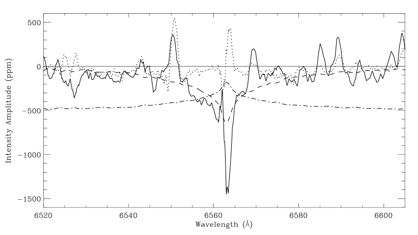
Figure 7: The solid line represents the relative intensity amplitude of the principal mode, while the other lines show three higher frequencies (harmonics).

Figure 8: The solid line represents the relative intensity cosine amplitude of the principal mode, this component represents intensity changes in phase or in anti-phase with the photometric pulsation. The dotted line represents the sine amplitude. The dashed line is a theoretical amplitude with $\delta I=-10^{-3}(C-I)$, and the dash-and-dotted line shows $\delta I=-5\times 10^{-4}I/C$ which represents approximately where the absolute flux amplitude would be zero (see text for details).

5.2 Results

The intensity amplitudes of the principal mode and harmonics, as a function of wavelength, are shown in Fig. 8. Note that a signal is expected in the first harmonic with an amplitude of about 8 percent of the principal mode (KSMT), with higher harmonics containing negligible signal. Therefore, the harmonics give a good indication of the noise level (the rms-noise is $\sim 60$ ppm). From Fig. 8, it is clear that the simple description of the profile variation given in Section 4.2 is inadequate and that the metal lines have an impact on the intensity variations. For instance, the peak blueward of H$\alpha$ could be caused by the Sr I 6550.2Å line, while the Fe I 6569.2Å line may also have an effect (this is more evident in the next figure). The signal from the core of H$\alpha$ is strong while the signal from the wings is much weaker.

To show the phase information, we have chosen to plot the cosine and sine components of the principal mode separately (see Fig. 8). The phase of most pixels is near 0° or 180°  and therefore most of the information is contained within the cosine component, which represents the relative intensity variations that are in phase or in anti-phase with the photometric pulsation. The amplitudes of this component are mostly negative which means that at maximum light, the relative intensity is at a minimum i.e. the EW of H$\alpha$ is at a maximum.

Two different simulations are also plotted:

1. The dashed line represents the relative intensity amplitude assuming $\delta I=-A(C-I)$, where $A$ is the EW amplitude of 1000 ppm. This is the amplitude (cosine component) expected from the profile variation described in Section 4.2.

2. The dash-and-dotted line represents $\delta I=-AI/C$ where $A$ is the continuum flux amplitude of 500 ppm (Medupe & Kurtz 1998). This line shows how the relative intensity amplitude (cosine component) would behave if the absolute flux in this region were constant (6520Å – 6605Å), and the continuum flux outside this region were pulsating at the measured value of 500 ppm. This is not a realistic simulation but we use it to estimate how the absolute flux in this region behaves. Where the solid line is above the dash-and-dotted line, the absolute flux is pulsating in phase with the continuum. We see that the absolute flux of the inner 10Å of the H$\alpha$ line is pulsating in anti-phase with the continuum.

5.3 Discussion

To evaluate these results, we have to consider systematic errors. Unlike for the bisector velocities, any systematic errors in the continuum level directly affect the EW and relative intensity measurements. The direction of any error would be the same at all wavelengths, equivalent to an offset in the cosine amplitude shown in Fig. 8. From looking at pseudo-continuum regions outside H$\alpha$, we estimate the intensity amplitude of the continuum level to be 100 ppm in the continuum fitted spectra (cosine component of $-$100 ppm). This slightly changes the details of the H$\alpha$  profile variation.

Other systematic errors may be caused by residual Doppler shift signals that were not removed by the reduction process. It was not possible to remove such signals completely because of the variation in velocity amplitude and phase between different lines and between different heights in the H$\alpha$  line. This could account for some of the sine component of the amplitude.

Ronan, Harvey & Duvall (1991) measured the oscillatory signal in the Sun as a function of optical wavelength. One of their wavelength regions included the Balmer lines H$\gamma$ and H$\delta$. More recently, Keller et al. (1998) looked at the H$\beta$ line region in the Sun, using a similar technique. Both groups showed that the absolute flux oscillations in the Balmer lines were reduced to about 70 percent of the continuum signal. This differs sharply from $\alpha$ Cir, where the H$\alpha$  core absolute flux is pulsating in anti-phase with the continuum. This may be due to a pulsational temperature node in the atmosphere of $\alpha$ Cir, as was indicated by the results of Medupe & Kurtz (1998), and by the velocity node. The relationship between the temperature node and the velocity node is unclear with the present data.

6 Detection of Other Frequencies

Figure 9: Amplitude ($\delta R_{cw}$) spectrum of the intensity ratio measurements.

In order to detect weaker modes in $\alpha$ Cir, we need an observable which has a high signal-to-noise ratio in the amplitude spectrum. Of the observables discussed so far, the one with the highest S/N for the principal mode is filter 2 from the EW measurements (S/N $=35$, see Col. 8 of Table 2). However, for the measurements of intensity in different filters across H$\alpha$, the noise level is approximately the same for filters 2–10 (20 ppm, see Col. 5 of Table 2). This means that the noise is caused by variations in the continuum level and not by photon noise. Therefore, we can improve the S/N for the principal mode by dividing the intensity in one filter by another and thereby reducing errors caused by the continuum fit. The highest S/N ($=51$) was obtained by dividing the intensity in filter 2 (FWHM $\sim 6$Å) by filter 7 (FWHM $\sim 45$Å). We call this observable $R_{cw}$ (ratio of H$\alpha$ core to wing intensity). This is analogous to narrow / wide H$\beta$ photometry.

Figure 10: Amplitude spectrum after subtracting the principal frequency. The dotted lines represent the frequencies of modes detected by KSMT.

Figure 11: Same as Fig. 11, at a higher frequency. The dotted line represents the frequency of the first harmonic of the principal mode. The inset shows the spectral window on the same frequency scale.

We produced a time series of these $R_{cw}$ measurements which was analysed in the same way as in Section 2.3. The amplitude ($\delta R_{cw}$) of the principal mode was measured to be 727 ppm, with an rms-noise level in the amplitude spectrum of 14 ppm (see Fig. 9). To search for other frequencies which were detected by KSMT (the same numbering is used), the principal pulsation mode was then subtracted from the time series to produce a pre-whitened amplitude spectrum (see Figs 11–11). In this spectrum, we have detected the modes $f_{4}$, $f_{5}$ and $2f_{1}$, and the rotational splitting of the principal mode ($f_{1}\pm r$), with amplitudes greater than $2.3\times$rms-noise. We have not measured the frequencies but have used the values given by KSMT, except we have increased the frequencies of $f_{1}$ to $f_{5}$ by 0.03 $\mu$Hz for consistency with the change in the principal frequency, as measured during our observations (see Paper I). The rotational splitting $r$ is taken as 2.59 $\mu$Hz, as measured by KSMT.

Table 3: The amplitudes ($\delta R_{cw}$) and phases of different modes measured using the intensity ratio of filter 2 and filter 7 (see Table 2). Except for the principal mode ($f_{1}$), the measurements are made after pre-whitening with the principal frequency.

mode	freq.a	ampl.	S/Nb	phasec	phase	relative amplitude
	($\mu$Hz)	(ppm)		(°)	errord	$\delta R_{cw}$e	photometricf
$f_{2}$	2265.46	26	1.8	279	33	0.036	0.055
$f_{3}$	2341.82	20	1.4	104	45	0.028	0.063
$f_{4}$	2366.97	35	2.4	272	24	0.048	0.057
$f_{1}-r$	2439.44	37	2.6	92	23	0.050	0.095
$f_{1}$	2442.03	727	50.8	174	1	1.000	1.000
$f_{1}+r$	2444.62	48	3.4	306	17	0.066	0.115
$f_{5}$	2566.52	34	2.4	16	25	0.047	0.046
$2f_{1}$	4884.06	48	3.4	76	17	0.066	0.077

^aFrequencies taken from KSMT. See text for details.
^brms-noise estimated to be 14 ppm from the pre-whitened amplitude spectrum in the region 1100–4400 $\mu$Hz.
^cPhase measured with respect to a reference-point ($t_{0}$) at JD 2450215.07527, with the convention that a phase of 0° represents maximum of the observed variable.
^dError in the phase is taken to be arcsin (rms-noise/amplitude).
^eError of approximately 0.020 (rms-noise/amplitude of principal mode).
^fStrömgren $v$ photometry (KSMT), with an error of approximately 0.007.

The amplitudes and phases of each mode are shown in Table 3, with the last two columns showing the amplitude relative to that of the principal mode, both for our spectral data and for KSMT’s photometric data. A possible significant difference is for the rotational side-lobes. Both side-lobes have a lower relative amplitude by more than 0.04 in our data. This rotational splitting is caused by a variation in the amplitude of the principal mode during the rotation cycle ($P_{\rm rot}=4.479$ days). Our results therefore suggest that the amplitude $\delta R_{cw}$ of the principal mode varies by less during the rotational cycle than the photometric amplitude.

To examine this, we divided the time series into 32 shorter time periods of about 4 hours each. In Fig. 13, we show the amplitude $\delta R_{cw}$ of the principal mode for each time period. The solid line shows the amplitude variation expected from the measurements of $f_{1}$, $f_{1}-r$ and $f_{1}+r$ in the amplitude spectrum of the complete time series (Table 3). The dotted line shows the expected amplitude variation based on the full range variation of 21 percent and the ephemeris from the photometric results (KSMT). There is good agreement between the amplitude maximum of our fit and the ephemeris of KSMT, which supports the accuracy of the rotation period derived by them. Both fits shown in Fig. 13 appear to be consistent with the results of the analysis using the shorter time periods. Therefore, we cannot say with certainty that the percentage amplitude variation is less in our data than the variation measured by KSMT. Such a difference, if it exists, may be due to limb-darkening.

The average value of $R_{cw}$ itself in each time period varied slightly during the observation period and was slightly different between the Stromlo and La Silla data sets (see Fig. 13). The difference in the value between the two data sets was about 0.4 percent and was due to the inexact matching of the filters. The variation with time seen in Fig. 13 is probably caused by the rotation of the star, which is slightly inhomogeneous in surface brightness. This variation does not significantly affect the measurement of $\delta R_{cw}$ at pulsation frequencies.

Variation of Balmer line profiles with rotation is common in Ap stars. For example, Musielok & Madej (1988) investigated 22 Ap stars of which 17 showed variation of the H$\beta$ index with a typical amplitude of 0.02 mag (19000 ppm). Our observed $\delta R_{cw}$ amplitude of about 1500 ppm at the rotation frequency in $\alpha$ Cir  corresponds to a much smaller Balmer line variation than is typical of Ap stars, even if we allow for some difference between the H$\beta$ index and $R_{cw}$. To test this, we calculated an intensity ratio using filters across H$\alpha$ of similar widths to those used for the H$\beta$ index (FWHMs $\sim 40$Å and $\sim 150$Å). The rotational amplitude of this intensity ratio was 1000–1500 ppm, which is more than a factor of ten smaller than the 0.02 mag found by Musielok & Madej in other Ap stars.

Figure 12: Amplitude ($\delta R_{cw}$) of the principal pulsation mode during separate time periods of approx. 4 hours. The asterisks represent the Stromlo data and the diamonds represent the La Silla data. The error bar for each amplitude measurement is the rms-noise level. See text for an explanation of the solid and dotted lines.

Figure 13: Average intensity ratio ($R_{cw}$) during separate time periods of approx. 4 hours. The asterisks represent the Stromlo data. The diamonds represent the La Silla data, which have been increased by 0.4 percent to match the Stromlo data. The dotted line shows a sine-wave with a period equal to the rotation period of the star.

7 Conclusions

The existence of a radial standing wave node of the principal pulsation mode has been put on a firm footing by the velocity phase reversal in the H$\alpha$ line. However, there is only a 140° velocity phase shift between the H$\alpha$ core and higher in the line. If we were seeing a pure standing wave in the atmosphere then we would expect a 180° phase shift. A travelling wave component, blending or the systematic effects described in Section 3.3 may cause the discrepancy. Additionally, many of the metal lines studied in Paper I show phases that are neither in phase or in anti-phase with the majority of the lines. We proposed that some of the phases were anomalous and did not represent velocity phases due to blending effects. Therefore, in a time series of less blended (higher resolution) spectra, there should be a clearer distinction between those lines that are formed above and below the velocity node and fewer lines with anomalous phases.

Analysis of the H$\alpha$ profile during the principal pulsation cycle, shows a large change in relative intensity of the core of the line. This means that the absolute flux of the core is pulsating in anti-phase with the continuum, indicating a pulsational temperature node in the atmosphere, as suggested by Medupe & Kurtz (1998) on the basis of multi-colour photometry. However, Medupe, Christensen-Dalsgaard & Kurtz (1998) show that non-adiabatic effects can explain the photometric results without the need for a node. Perhaps, non-adiabatic effects have a significant effect on the H$\alpha$ profile changes in $\alpha$ Cir.

The next stage in the analysis of the mode dynamics in the atmosphere could be the use of high resolution (R$\sim$50000) spectroscopy to study the velocities, bisectors and EW changes of unblended metal lines, combined with model atmospheres to calculate the formation height of the lines. This may allow us to decide whether there is travelling wave component, to relate the velocity changes to the temperature changes, to measure any surface or vertical inhomogeneities in the distribution of certain elements, and to test non-adiabatic non-radial pulsation equations.

By defining an observable which detects the relative intensity changes in the core of the H$\alpha$ line, $R_{cw}$, we detected some of the weaker modes in $\alpha$ Cir. This is probably the first detection, in roAp stars, of modes with photometric ($B$) amplitudes of less than 0.2 mmag, using a spectroscopic technique. The ratio between spectroscopic amplitudes and photometric amplitudes can be used to identify the $\ell$ value of different oscillations modes, as has been done recently by Viskum et al. (1998) for the $\delta$ Scuti star FG Vir. We do not have enough S/N to identify the modes in $\alpha$ Cir, but we show the potential for using this mode identification technique.

$\alpha$ Cir offers one of the best chances for theoreticians to model a star where magnetic fields are important both for its evolution and pulsation, because of the detailed information that can be gained from its oscillation modes using spectroscopy and photometry. Additionally, there is already a well determined luminosity using Hipparcos and, when angular diameter measurements are made, there will also be direct measurements of the effective temperature and radius of the star.

8 Acknowledgements

Many thanks to Jaymie Matthews and Don Kurtz, with whom we had fruitful discussions, and to Friedrich Kupka and DK for providing data on $\alpha$ Cir. Thanks also to Thebe Medupe and Lawrence Cram for help with the model atmospheres. We are grateful to Michael Bessell for his help and advice in setting up the instrument at Mt. Stromlo, and to the Director of Mt. Stromlo Observatory and the Danish Time Allocation Committee for the telescope time. We acknowledge the Harvard ADS Abstract Service as an invaluable aid in finding relevant papers.

This work was carried out while IKB was in receipt of an Australian Postgraduate Award, and was also supported by funds from the Australian Research Council, the Danish Natural Science Research Council through its Center for Ground-based Observational Astronomy, and the Danish National Research Foundation through its establishment of the Theoretical Astrophysics Center.

References

- [1] Baldry I.K., Bedding T.R., Viskum M., Kjeldsen H., Frandsen S., 1998a, MNRAS, 295, 33 (Paper I)
- [2] Baldry I.K., Bedding T.R., Viskum M., Kjeldsen H., Frandsen S., 1998b, in Deubner F.-L., Christensen-Dalsgaard J., Kurtz D.W., eds, Proc. IAU Symp. 185, New Eyes to See Inside the Sun and Stars. Kluwer, Dordrecht, p. 309
- [3] Bedding T.R., Kjeldsen H., Reetz J., Barbuy B., 1996, MNRAS, 280, 1155
- [4] Brown T.M., Gilliland R.L., 1994, ARA&A, 32, 37
-
[5]
Christensen-Dalsgaard J., 1998,
Lecture Notes on Stellar Oscillations. Univ. Aarhus
(http://www.obs.aau.dk/~jcd/oscilnotes/) - [6] Deubner F.-L., Waldschik Th., Steffens S., 1996, A&A, 307, 936
- [7] ESA, 1997, The Hipparcos and Tycho Catalogues. ESA SP-1200
- [8] Gautschy A., Saio H., Harzenmoser H., 1998, MNRAS, submitted
- [9] Hatzes A.P., 1996, PASP, 108, 839
- [10] Keller C.U., Harvey J.W., Barden S.C., Giampapa M.S., Hill F., Pilachowski C.A., 1998, in Deubner F.-L. et al., eds, New Eyes to See Inside the Sun and Stars. Kluwer, Dordrecht, p. 375
- [11] Kjeldsen H., Bedding T.R., 1995, A&A, 293, 87
- [12] Kjeldsen H., Bedding T.R., Viskum M., Frandsen S., 1995, AJ, 109, 1313
- [13] Kupka F., Ryabchikova T.A., Weiss W.W., Kuschnig R., Rogl J., Mathys G., 1996, A&A, 308, 886
- [14] Kurtz D.W., 1982, MNRAS, 200, 807
- [15] Kurtz D.W., Sullivan D.J., Martinez P., Tripe P., 1994, MNRAS, 270, 674 (KSMT)
- [16] Kurucz R.L., 1979, ApJS, 40, 1
- [17] Medupe R., Kurtz D.W., 1998, MNRAS, 299, 371
- [18] Medupe R., Christensen-Dalsgaard J., Kurtz D.W., 1998, in Bradley P.A., Guzik J.A., eds, ASP Conf. Ser. Vol. 135, A Half Century of Stellar Pulsation Interpretations. Astron. Soc. Pacific, San Francisco, p. 197
- [19] Musielok B., Madej J., 1988, A&A, 202, 143
- [20] Ronan R.S., Harvey J.W., Duvall T.L. Jr., 1991, ApJ, 369, 549
- [21] Schmidt-Kaler Th., 1982, in Schaifers K., Voigt H.H., eds, Landolt-Börnstein: Numerical Data and Functional Relationships in Science and Technology, Group VI, Vol. 2b. Springer-Verlag, Berlin, p. 451
- [22] Shibahashi H., Takata M., 1993, PASJ, 45, 617
- [23] Viskum M., Kjeldsen H., Bedding T.R., Dall T.H., Baldry I.K., Bruntt H., Frandsen S., 1998, A&A, 335, 549