Gamma-ray bursts from accreting black holes in neutron star mergers

Abstract

By means of three-dimensional hydrodynamic simulations with a Eulerian PPM code we investigate the formation and the properties of the accretion torus around the stellar mass black hole which originates from the merging of two neutron stars. The simulations are performed with four nested cartesian grids which allow for both a good resolution near the central black hole and a large computational volume. They include the use of a physical equation of state as well as the neutrino emission from the hot matter of the torus. The gravity of the black hole is described with a Newtonian and alternatively with a Paczyński-Wiita potential. In a post-processing step, we evaluate our models for the energy deposition by $\nu\bar{\nu}$ annihilation around the accretion torus.

We find that the torus has a mass between several $10^{-2}\,M_{\odot}$ and a few $10^{-1}\,M_{\odot}$ with maximum densities around $10^{12}\,{\rm g\,cm}^{-3}$ and maximum temperatures of about $10\,$MeV (entropies around 5$\,k_{\rm B}$ per nucleon). Correspondingly, the neutrino emission is huge with a total luminosity near $10^{53}\,{\rm erg\,s}^{-1}$. Neutrino-antineutrino annihilation deposits energy in the vicinity of the torus at a rate of (3–$5)\times 10^{50}\,{\rm erg\,s}^{-1}$. It is most efficient near the rotation axis where 10 to 30% of this energy or up to a total of $10^{49}\,{\rm erg}$ are dumped within an estimated emission period of 0.02–0.1 s in a region with a low integral baryonic mass of about $10^{-5}\,M_{\odot}$. This baryon pollution is still dangerously high, and the estimated maximum relativistic Lorentz factors $\Gamma-1$ are around unity. The conversion of neutrino energy into a pair plasma, however, is sufficiently powerful to blow out the baryons along the axis so that a clean funnel should be produced within only milliseconds. Our models show that $\nu\bar{\nu}$ annihilation can yield the energy to account for weak, short gamma-ray bursts, if moderate beaming is involved. In fact, the barrier of the dense baryonic gas of the torus suggests that the low-density $e^{\pm}\gamma$ plasma is beamed as axial jets into a fraction $f_{\Omega}=2\delta\Omega/(4\pi)$ between $1/100$ and $1/10$ of the sky, corresponding to opening half-angles of roughly ten to several tens of degrees. Thus $\gamma$-burst energies of $E_{\gamma}\approx E_{\nu\bar{\nu}}/f_{\Omega}\mathrel{\vbox{\offinterlineskip\hbox{$<$}\hbox{$\sim$}}}10^{50}$–$10^{51}\,$erg seem within the reach of our models (if the source is interpreted as radiating isotropically), corresponding to luminosities around $10^{51}\,{\rm erg\,s}^{-1}$ for typical burst durations of 0.1–1 s. Gravitational capture of radiation by the black hole, redshift and ray bending do not reduce the jet energy significantly, because most of the neutrino emission comes from parts of the torus at distances of several Schwarzschild radii from the black hole. Effects associated with the Kerr character of the rapidly rotating black hole, however, could increase the $\gamma$-burst energy considerably, and effects due to magnetic fields might even be required to get the energies for long complex gamma-ray bursts.

1 Introduction

In a sequence of preceding papers (Ruffert et al. ruf96 (1996), ruf97 (1997); Ruffert & Janka 1998a ; 1998b ) we have shown that the neutrino emission associated with the dynamical phase of the merging or collision of two neutron stars is powerful, but too short to provide the energy for gamma-ray bursts by neutrino-antineutrino annihilation. Significant heating of the coalescing stars occurs only after they have plunged into each other, and the neutrino luminosities can rise to several $10^{53}\,{\rm erg\,s}^{-1}$ and even exceed $10^{54}\,{\rm erg\,s}^{-1}$ in case of the more violent collisions. After a few milliseconds, however, the compact massive remnant of the merger will most likely collapse to a black hole. If that did not happen, the remnant’s continuing neutrino emission would drive a dense baryonic wind off its surface which would lead to a sizable mass loss but non-relativistic expansion (Woosley & Baron woo92 (1992), Woosley 1993b , Hernanz et al. her94 (1994), Qian & Woosley qia96 (1996)), a situation which is not favorable for producing gamma-ray bursts which require relativistic Lorentz factors $\Gamma\mathrel{\vbox{\offinterlineskip\hbox{$>$}\hbox{$\sim$}}}100$ (Paczyński pac90 (1990)).

If the merger remnant collapses to a black hole, some matter remains in an accretion disk or torus around the black hole. Our hydrodynamic simulations (Ruffert et al. ruf96 (1996), Ruffert & Janka 1998b ) have given hints that about $0.1\,M_{\odot}$ of matter might obtain enough angular momentum during the merging of the neutron stars to resist immediate collapse into the black hole. In this case a funnel with low baryon density can develop along the system axis. On the other hand, the large angular momentum ensures that the torus matter is swallowed by the black hole on a time scale much longer than the dynamical time scale. Therefore there could be enough time for this material to radiate away a fair fraction of its gravitational binding energy in neutrinos, even if the densities become so high that neutrinos get trapped and can escape only on a diffusion time scale. A similar situation could result from the merging of a neutron star with a black hole (Lee & Kluźniak lee95 (1995, 1998); Kluźniak & Lee klu98 (1998); Eberl 1998a ; Eberl et al. 1998b ), from the collapse of a very massive, rapidly rotating star (Woosley 1993a , Popham et al. pop98b (1998), MacFadyen & Woosley mac98 (1998)), or from the coalescence of a neutron star/black hole with a white dwarf (Fryer et al. fry98b (1998)) or with the helium core of its red giant companion (Fryer & Woosley fry98a (1998)).

All these events are estimated to occur at rates which can account for the observed frequency of gamma-ray bursts (about one burst per day). Also, the huge amount of gravitational binding energy released during the accretion process of up to several solar masses of gas into the black hole is hoped to be able to explain the energetics of even the most distant cosmological gamma-ray bursts (e.g., GRB981214, see Kulkarni et al. kul98 (1998)). Moreover, the compactness of the stellar-mass black hole could naturally produce the rapid variability on time scales of milliseconds observed in many bursts. For these reasons, massive accretion disks or thick accretion tori around stellar-mass black holes are considered as possible cosmological origin of the enigmatic gamma-ray bursts, powered by neutrino-antineutrino annihilation or by magnetically driven energy release (e.g., Paczyński pac86 (1986); Goodman goo86 (1986); Goodman et al. goo87 (1987); Eichler et al. eic89 (1989); Paczyński pac91 (1991); Narayan et al. nar92 (1992); Mészáros & Rees mes93 (1993); Woosley 1993a ; Jaroszyński jar93 (1993, 1996); Mochkovitch et al. moc93 (1993, 1995); Thompson tho94 (1994); Witt et al. wit94 (1994); Janka & Ruffert jan96 (1996); Mészáros & Rees mes97 (1997); Popham et al. pop98b (1998); Mészáros et al. mes98 (1998)).

In this paper we simulate the formation of the accretion torus after two neutron stars have merged, and assume that the compact remnant with a baryonic mass of about $3\,M_{\odot}$ has collapsed into a black hole. The initial model is taken from our merger simulations (Ruffert & Janka 1998b ) where the central, massive object is replaced by a vacuum boundary at a radius equal to twice the Schwarzschild radius of the mass dumped into the black hole. We follow the evolution of the left-over material in the surroundings of the black hole until it either has settled into the disk or has been swallowed by the black hole. At the end of our three-dimensional computations, the torus has reached a quasi-stationary state and its further evolution is governed by the viscous transport of angular momentum which depends on the uncertain value of the disk viscosity. Kerr effects associated with the rotation of the black hole and magnetic fields are not taken into account in our models. An extensive, general investigation of relativistic steady-state accretion from tori around hyper-accreting stellar black holes for different accretion rates and disk viscosities in Schwarzschild and Kerr geometry was recently published by Popham et al. (pop98b (1998)). Our simulations focus on the situation that emerges from the mergings of compact binary systems of neutron stars and black holes, and they are intended to help constrain the large parameter space and to yield insight into the torus properties and non-stationary aspects of the evolution.

In particular, our simulations aim at answering the following questions: How much mass remains in the accretion torus? What is the relativistic rotation parameter $a\equiv Jc/(GM^{2})$ of the black hole? What are the properties of the accretion torus, its density, temperature, neutrino luminosity? How much mass pollutes the surroundings of the accretion torus, in particular, does an effectively baryon-free funnel form along the system axis? How efficient is neutrino-antineutrino annihilation in depositing energy in the regions with low baryon density? Can we make estimates of the mass accretion rate into the black hole and the corresponding lifetime of the torus? What are the implications for producing gamma-ray bursts by neutrino-antineutrino annihilation? Is pair-plasma ejected in a jet and how large will its opening angle be? Is there enough variability of the energy release at the central source to account for the observed time structure of the gamma-ray burst light curves?

The paper is organized as follows. In Sect. 2 the computational procedures are summarized which are used in our simulations of the torus formation after neutron star merging. The initial model for these simulations is briefly described and the different investigated cases are introduced with their distinguishing parameters. Section 3 contains a description of the dynamical evolution of the torus from the beginning of the simulations until a quasi-stationary state was reached. In Sect. 4 the properties of the accretion tori at the end of the computations are described. The results on the neutrino emission are presented in Sect. 5 and those for neutrino-antineutrino annihilation in Sect. 6. In Sect. 7 the hydrodynamic results are used to estimate the numerical viscosity which determines our torus models; the general relativistic effects in the neutrino-antineutrino annihilation are discussed as well as the importance of neutrino-electron/positron scattering for the heating of the pair-plasma cloud that is formed by $\nu\bar{\nu}$ annihilation. Section 8 concludes the paper with a summary and a discussion of the implications of our results for gamma-ray burst scenarios involving massive accretion tori around stellar mass black holes.

Table 1: Some parameters for the torus evolution models with Newtonian potential (Models B1, B2, B4, and B10) and with Paczyński-Wiita potential (Models ${\cal B}$1, ${\cal B}$2, and ${\cal B}$10), respectively. The dynamical simulations were started with initial conditions as given from Model B64 of Ruffert & Janka (1998b ) at different times $t_{\rm init}$ and the evolutions were followed over time intervals $\Delta t_{\rm cal}$. All other quantities refer to the conditions found at the end of the simulations. $M_{\rho<11}$ is the mass on the grid with density less than $10^{11}\,{\rm g\,cm}^{-3}$, $M_{\rm v}$ the total gas mass on the computational grid, and $M_{\rm d}$ the mass of the gas with specific angular momentum larger than the Kepler limit $j^{*}_{\rm N}\equiv v_{\rm Kepler}^{\rm N}(3R_{\rm s})3R_{\rm s}=\sqrt{6}GM/c$ in case of the Newtonian potential or $j^{*}_{\rm PW}\equiv v_{\rm Kepler}^{\rm PW}(3R_{\rm s})3R_{\rm s}={3\over 2}j^{*}_{\rm N}$ for the Paczyński-Wiita potential; the Kepler velocities were evaluated from Eqs. (5) and (6) using for $M$ the sum of black hole and total gas mass on the grid at the end of the simulation. $T_{\rm max}$ is the maximum gas temperature in energy units. $L_{\nu_{e}}$ denotes the electron neutrino luminosity near the end of the simulation, $L_{\bar{\nu}_{e}}$ the corresponding electron antineutrino luminosity, and $L_{\nu_{x}}$ the luminosity of each individual flavor of heavy-lepton neutrino ($\nu_{\mu}$, $\bar{\nu}_{\mu}$, $\nu_{\tau}$ or $\bar{\nu}_{\tau}$). The sum of all individual neutrino luminosities is given by $L_{\nu}$, and the mean energies of the different neutrino types by $\langle\epsilon_{\nu_{e}}\rangle$, $\langle\epsilon_{\bar{\nu}_{e}}\rangle$ and $\langle\epsilon_{\nu_{x}}\rangle$.

model	potential	$t_{\rm init}$	$\Delta t_{\rm cal}$	$M_{\rho<11}$	$M_{\rm v}$	$M_{\rm d}$	$T_{\rm max}$	$L_{\nu_{e}}$	$L_{\bar{\nu}_{e}}$	$L_{\nu_{x}}$	$L_{\nu}$	$\langle\epsilon_{\nu_{e}}\rangle$	$\langle\epsilon_{\bar{\nu}_{e}}\rangle$	$\langle\epsilon_{\nu_{x}}\rangle$
		ms	ms	$10^{-2}M_{\odot}$	$10^{-2}M_{\odot}$	$10^{-2}M_{\odot}$	MeV	$10^{52}\frac{\rm erg}{\rm s}$	$10^{52}\frac{\rm erg}{\rm s}$	$10^{52}\frac{\rm erg}{\rm s}$	$10^{52}\frac{\rm erg}{\rm s}$	MeV	MeV	MeV
B1	Newt	1.84	2.5	4.6	23.2	16.3	7.	0.3	0.7	0.002	1.0	7.	13.	15.
B2	Newt	2.60	1.7	6.8	36.2	28.6	8.	0.4	0.8	0.003	1.2	8.	13.	14.
B4	Newt	4.09	5.0	4.8	26.7	22.0	9.	2.2	5.6	0.033	8.0	9.	14.	18.
B10	Newt	10.0	4.9	6.3	26.4	24.2	12.	3.5	6.5	0.40	12.	9.	13.	21.
${\cal B}$1	PaWi	1.84	3.2	0.5	0.5	0.16	4.	0.02	0.12	0.0001	0.14	12.	12.	10.
${\cal B}$2	PaWi	2.60	6.0	2.8	3.4	2.4	7.	2.0	4.5	0.017	6.5	11.	16.	17.
${\cal B}$10	PaWi	10.0	5.2	2.0	3.5	3.1	8.	2.5	4.0	0.04	6.7	10.	16.	15.

2 Computational procedures, initial conditions and different models

In Ruffert & Janka (1998b ) we have calculated a series of neutron stars merger models with varied neutron star masses, neutron star mass ratios, neutron star spins, and initial conditions (temperature, entropy) in the coalescing stars. In all of these simulations the post-merging configuration consisted of a compact central object with a mass of about $3\,M_{\odot}$ and a typical density of the order of $10^{14}\,{\rm g\,cm}^{-3}$ which was surrounded by an extended cloud of more dilute gas, having a mass of a few $0.1\,M_{\odot}$ and a characteristic mean density around $10^{11}$–$10^{12}\,{\rm g\,cm}^{-3}$. To estimate the gas mass which might be able to stay in an accretion torus after the massive object has collapsed into a black hole, we compared the specific angular momentum $j$ of the matter to the Keplerian angular momentum $j^{*}$ for a test particle with non-zero mass that orbits around the Schwarzschild black hole on the last stable circular orbit at 3 Schwarzschild radii, $3R_{\rm s}=6GM/c^{2}$. Taking for simplicity $M$ as the total (gas) mass on the grid, we found that between several $10^{-2}\,M_{\odot}$ and a few $10^{-1}\,M_{\odot}$ fulfill this criterion : $j>j^{*}_{\rm N}\equiv v_{\rm Kepler}^{\rm N}(3R_{\rm s})3R_{\rm s}=\sqrt{6}GM/c$ where $v_{\rm Kepler}^{\rm N}$ is the Keplerian velocity and the superscript (or subscript) N indicates the use of a Newtonian gravitational potential. The amount of mass which has sufficiently large angular momentum to resist immediate (i.e., on a dynamical time scale) accretion into the black hole depends on the neutron star masses and mass ratio as well as on the neutron star spins which contribute to the total angular momentum of the binary system. For the simulations of the formation of the accretion torus which we describe in this paper, the neutron star merger Model B64 of Ruffert & Janka (1998b ) was used as an initial condition (defined by the distributions of density, temperature and electron fraction, and by the velocity field at a certain chosen time during the evolution of Model B64). Due to the assumed corotation of the two $1.6\,M_{\odot}$ (baryonic mass) neutron stars before merging, the angular momentum was largest in this model and correspondingly, the estimated possible torus mass was maximal.

The three-dimensional computations of neutron star mergings were performed with a Newtonian hydrodynamics code based on the Piecewise Parabolic Method (PPM) of Colella & Woodward (col84 (1984)) with at least four levels of nested grids (Ruffert ruf92 (1992)) to ensure both high resolution at the neutron stars and a large computational volume. The code includes the effects of gravitational-wave emission and their back-reaction on the hydrodynamic flow according to Blanchet et al. (bla90 (1990)) (see Ruffert et al. ruf96 (1996)). In addition, we implemented a calibrated neutrino leakage scheme (Ruffert et al. ruf96 (1996)) in order to calculate the energy and lepton number loss by neutrino emission from the heated neutron star matter. The latter is described by the finite-temperature nuclear equation of state of Lattimer & Swesty (lat91 (1991)) using the Sk180 nuclear force parameter set (Swesty et al. swe94 (1994)).

Figure 1: Maximum absolute value of the gravitational potential produced by the mass distribution of Model B64 of Ruffert & Janka (1998b ) as function of time, normalized to $c^{2}$. This parameter, multiplied by 2, is a measure of the importance of relativistic corrections, and is very small in the limit of Newtonian gravity. The time is measured from the beginning of the simulation of the neutron star merger Model B64.

The torus simulations presented in this paper are done with the same code and the same input physics. Because of the spherical symmetry of the mass in the black hole and the relatively small mass of the accretion torus, time derivatives of the quadrupole moment are small and gravitational-wave production does not play an important role. Although taken into account in our simulations, we shall therefore not report data of the gravitational-wave emission here. In one set of our models (B1, B2, B4, and B10) the black hole potential, which dominates the gravitational field at the torus (whose self-gravity is only a minor contribution), is represented by a Newtonian potential,

$$\Phi_{\rm N}\,=\,-{GM_{\rm BH}\over r}\ .$$ (1)

In a second sequence of models (${\cal B}$1, ${\cal B}$2, and ${\cal B}$10) the gravitational potential is described by the Paczyński-Wiita expression,

$$\Phi_{\rm PW}\,\equiv\,-{GM_{\rm BH}\over r-R_{\rm s}}$$ (2)

(Paczyński & Wiita pac80 (1980)). This allows one to reproduce the existence and the effects of a last stable circular orbit at a radius of $3R_{\rm s}=6GM_{\rm BH}/c^{2}$ where the specific angular momentum $j_{\rm PW}=rv_{\rm Kepler}^{\rm PW}(r)=\sqrt{GM_{\rm BH}r^{3}/(r-R_{\rm s})^{2}}$ has an absolute minimum. We hope that this approximation, although crude, can give us some indication of the sensitivity of our results to the inclusion of proper general relativity in the modeling.

Figure 2: Distribution of mass and angular momentum in the remnant of the neutron star merger of Model B64 of Ruffert & Janka (1998b ) at time $t=10\,$ms. This defines the initial condition used for some of the torus simulations presented here. The upper thin solid line gives the cumulative gas mass (in solar masses), the lower thin solid line the cumulative angular momentum (in $10^{49}\,{\rm g\,cm}^{2}\,{\rm s}^{-1}$), and the thick solid line the relativistic rotation parameter $a(r)\equiv J(r)c/(GM_{\rm gas}^{2}(r))$ as functions of radius $r$. ($M_{\rm gas}(r)$ is the gas mass inside $r$ and $J(r)$ the corresponding angular momentum perpendicular to the equatorial plane.)	Figure 3: Mass accretion rates of the black hole (in $M_{\odot}\,{\rm ms}^{-1}$) as functions of time for all models listed in Table 1. The thick lines which start at times $t=1.84\,{\rm ms}$, $2.60\,{\rm ms}$, $4.09\,{\rm ms}$, and $10.0\,{\rm ms}$ correspond to the Newtonian Models B1, B2, B4, and B10, respectively, and the thin lines starting at times $t=1.84\,{\rm ms}$, $2.60\,{\rm ms}$, and $10.0\,{\rm ms}$ correspond to Models ${\cal B}1$, ${\cal B}2$, and ${\cal B}10$, respectively.
Figure 4: The mass of the central black hole as function of time for Model B10 (bold line) and Model ${\cal B}$10 (thin line), showing an increase due to accretion of surrounding gas.	Figure 5: Typical time scales for the changes of black hole mass (solid lines) and torus mass (dashed lines) as functions of time for Model B10 (bold lines) and Model ${\cal B}$10 (thin lines).

Figure 6: Different masses as functions of time for the Newtonian Models B1, B2, B4, and B10 (left plot) and for the different Paczyński-Wiita Models ${\cal B}$1, ${\cal B}$2, and ${\cal B}$10 (right plot) (distinguishable by their start and stop times, see Table 1). $M_{\rm v}$ (bold solid lines) denotes the gas mass on the grid, $M_{\rm u}$ (dashed lines) is the cumulative mass which leaves the grid during the simulation and becomes unbound, i.e., which fulfils the criterion that its total specific energy as the sum of its specific internal, kinetic, and potential energies is positive. The dotted curves with labels $M_{10}$, $M_{11}$, and $M_{12}$ show the gas masses with densities below $10^{10}\,{\rm g\,cm}^{-3}$, $10^{11}\,{\rm g\,cm}^{-3}$, and $10^{12}\,{\rm g\,cm}^{-3}$, respectively. In case of the Newtonian potential (left plot), the thin solid lines labeled with $M_{\rm d}$ represent the mass on the grid with specific angular momentum larger than the Kepler value at 3 Schwarzschild radii, i.e., $j\geq j_{\rm N}^{\ast}=\sqrt{6}GM/c$, where for $M$ the sum of the black hole mass and gas mass on the grid was used at all times.

Figure 7: Maximum density on the grid as function of time for the Newtonian Models B2, B4, and B10 (bold lines) and for the Paczyński-Wiita Models ${\cal B}$2 and ${\cal B}$10 (thin lines).	Figure 8: Maximum temperature on the grid as function of time for the Newtonian Models B2, B4, and B10 (bold lines) and for the Paczyński-Wiita Models ${\cal B}$2 and ${\cal B}$10 (thin lines).

Figure 9: Average value of the specific internal energy of the matter on the grid as function of time for Model B10 (bold line) and Model ${\cal B}$10 (thin line).	Figure 10: Total kinetic, thermal, and gravitational potential energies as functions of time for Model B10 (bold line) and Model ${\cal B}$10 (thin line).

The different models of each set, B# and ${\cal B}$#, respectively, are discerned by the different times $t_{\rm init}$ (in milliseconds given by the numbers in the model names) at which the compact object that formed during the merging of the two neutron stars in Model B64 of Ruffert & Janka (1998b ) was removed and replaced by a gravitating “vacuum sphere”. The times $t_{\rm init}$ are measured from the start of the simulation of Model B64 and are listed in Table 1. If a black hole forms from the compact central body of the merger remnant with a baryonic mass of nearly $3\,M_{\odot}$, we expect this to happen at about the time when the most compact state is reached and thus the gravitational potential becomes strongest. If support by centrifugal forces or thermal pressure played a role, the collapse might be delayed. Figure 1 shows that the value of the parameter $\Phi_{\rm N}/c^{2}$ — twice of which gives a rough measure for the importance of general relativistic gravity — plateaus at about $2\,$ms after the simulation of the merging of the neutron stars was started. Therefore we chose the earliest moment of the possible black hole formation and the onset of our torus computations at around this time, and investigated also models for later collapse times at about $4\,$ms and $10\,$ms, respectively. The model runs were continued until the accretion rate into the black hole had reached such a low value that further changes of the torus properties would happen over a much longer period than the dynamical time scale of the system. The computed evolution times $\Delta t_{\rm cal}$ of all models are also given in Table 1. The subsequent quasi-stationary evolution proceeds on the time scale of viscous transport of angular momentum which depends on the unknown value of the disk viscosity and in general is too long to be followed by our three-dimensional, hydrodynamic simulations with an explicit code.

The inner vacuum sphere that represents the black hole at the center of the computational grid is set to a radius of $2R_{\rm s}$. The Schwarzschild radius $R_{\rm s}$ is initially computed for 90% of the total gas mass on the grid and the mass of the gas inside this radius is collected into the black hole to determine its gravitational potential. During the following evolution, the black hole mass, momentum and angular momentum are updated by adding the corresponding values of the matter which is advected through the sphere at $2R_{\rm s}$. From the current value of the black hole mass, the new radius of the vacuum sphere and the new gravitational potential of the black hole are calculated. The loss of mass, momentum, angular momentum and energy from the gas outside the black hole boundary are also monitored during the simulations. In the grid zones that are located inside the vacuum sphere (these zones are not removed from the hydrodynamic grid), the mass density is continuously reset to a negligibly small but finite value of $10^{8}\,{\rm g\,cm}^{-3}$ and a correspondingly very small value of the pressure is used. The decision to put the vacuum boundary at the radius $2R_{\rm s}$ was influenced by the facts that on the one hand the gravitational potential in the Paczyński-Wiita case diverges when $r$ decreases towards $1R_{\rm s}$, and that on the other hand the gas velocities come close to the speed of light already near $2R_{\rm s}$ and therefore the nonrelativistic treatment of the hydrodynamics can definitely not be applied any longer. Moreover, the Courant-Friedrich-Lewy timestep of the explicit computation is limited by the small values in this region on the finest grid. From a physics point of view, the choice of the black hole boundary at $2R_{\rm s}$ can be justified because the generated black hole is not of extreme Kerr type but its relativistic rotation parameter $a$ is of order 0.4–0.5 (Fig. 5). In this case the inner edge of the torus should be located at just around two times the horizon radius (see Usui et al. usu98 (1998)). Interior to this radius the orbits are unstable and the infall velocities become very large, i.e., the matter moves essentially radially inward. Our Newtonian code does not take into account effects due to the rotation of the black hole on the surrounding space and matter, e.g., frame dragging or the dependence of the radius of the innermost stable orbit on the rotation parameter of the black hole.

The simulations are performed with four levels of nested cartesian grids, each having 64 zones per dimension in the orbital plane and 16 perpendicular to the orbital plane (here we make use of equatorial symmetry and of the smaller extension of the torus in the vertical direction). A zone on the finest grid has a length of $\Delta x=\Delta y=\Delta z=0.64\,$km, and the size of the largest grid is $328\,{\rm km}\times 328\,{\rm km}\times 82\,{\rm km}$.

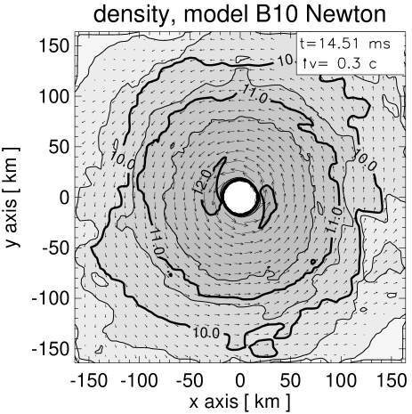
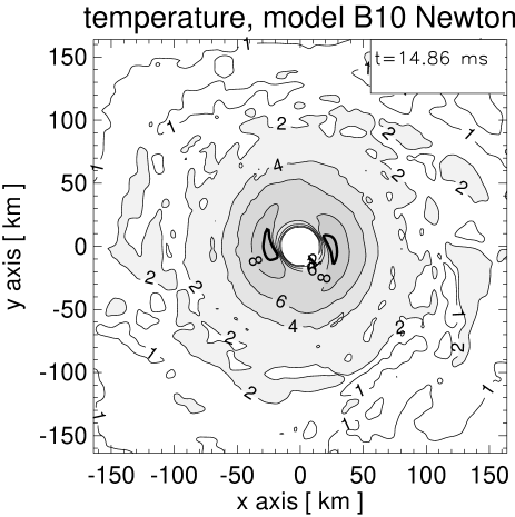
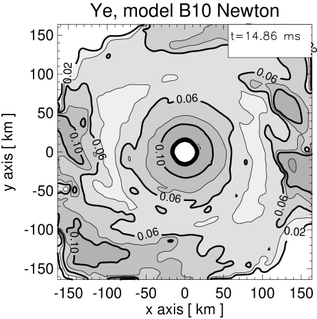
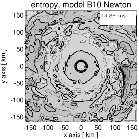
Figure 11: Structure of the Newtonian Model B10 in the equatorial plane near the end of the simulation. Panel a shows contours of the baryonic mass density (measured in ${\rm g\,cm}^{-3}$) together with the flow field indicated by velocity vectors, panel b displays contours of the temperature (in MeV), panel c of the electron fraction $Y_{e}$, and panel d of the entropy per nucleon. The length scale of the velocity vectors and the time elapsed since the beginning of the simulation of Model B64 of Ruffert & Janka (1998b ) are given in the insert in the top right corner of the figures. The density contours are spaced logarithmically with intervals of 0.5 dex (bold: $\log(\rho\left[{\rm g\,cm}^{-3}\right])=10.0,\,11.0,\,12.0$), the temperature contours are spaced linearly, starting with 1 MeV and 2 MeV, and then continuing in steps of 2 MeV (bold: $T=10\,{\rm MeV}$), the $Y_{e}$ contours are spaced linearly with intervals of 0.02 (bold: 0.02, 0.06, 0.10, 0.16), and the entropy levels were chosen to be 1, 2, 3, 4, 5, 6, 8, 10, 12, 14, 16, and 20 (bold: 6, 10, 20). Some of the contours are labeled with their respective values, and darker grey shading indicates higher values of a quantity. The circle around the center marks the inner “vacuum” boundary with semidiameter of twice the Schwarzschild radius for the mass which has accumulated in the central black hole.

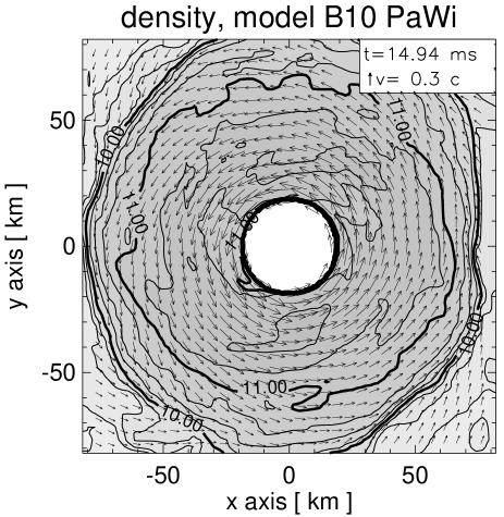
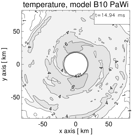
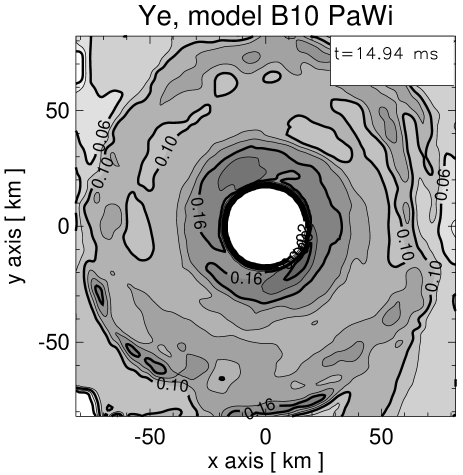
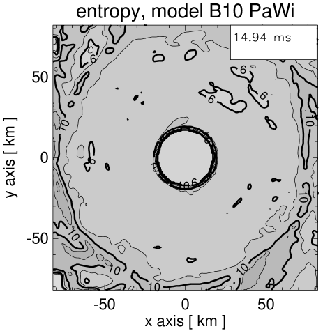
Figure 12: Structure of the Paczyński-Wiita Model ${\cal B}$10 in the equatorial plane near the end of the simulation. Panel a shows contours of the baryonic mass density (measured in ${\rm g\,cm}^{-3}$) together with the flow field indicated by velocity vectors, panel b displays contours of the temperature (in MeV), panel c of the electron fraction $Y_{e}$, and panel d of the entropy per nucleon. The length scale of the velocity vectors and the time elapsed since the beginning of the simulation of Model B64 of Ruffert & Janka (1998b ) are given in the insert in the top right corner of the figures. The density contours are spaced logarithmically with intervals of 0.25 dex (bold: $\log(\rho\left[{\rm g\,cm}^{-3}\right])=10.0,\,11.0$), the temperature contours are spaced linearly, starting with 1 MeV and 2 MeV and then continuing in steps of 2 MeV (bold: $T=10\,{\rm MeV}$), the $Y_{e}$ contours are spaced linearly with intervals of 0.02 (bold: 0.02, 0.06, 0.10, 0.16), and the entropy levels were chosen to be 1, 2, 3, 4, 5, 6, 8, 10, 12, 14, 16, and 20 (bold: 6, 10, 20). Some of the contours are labeled with their respective values, and darker grey shading indicates higher values of a quantity. The circle around the center marks the inner “vacuum” boundary with semidiameter of twice the Schwarzschild radius for the mass which has accumulated in the central black hole.

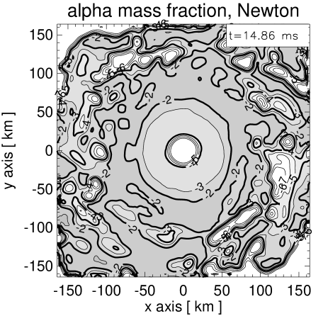
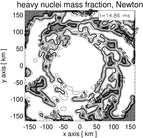
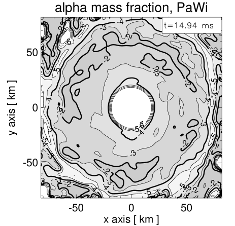
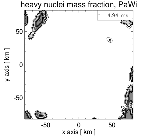
Figure 13: Contour plots of the mass fractions of $\alpha$ particles and heavy nuclei in the equatorial plane of Model B10 (panels a and b, respectively) and of Model ${\cal B}$10 (panels c and d, respectively) at the times given in the inserts in the top right corners of the figures. The contours are spaced logarithmically with steps of $-1$ (starting at $-7$; bold lines for levels $-4$ and $-2$) in case of the $\alpha$ mass fraction and with levels $-8$, $-6$, $-4$, $-2$, $-1.5$, $-1$, $-0.8$, $-0.6$, $-0.4$, $-0.2$ and 0 (bold lines for levels $-6$ and $-1$) in case of heavy nuclei. Typical mass numbers $A$ of heavy nuclei are around 80–120 with charge numbers $Z\approx 25$–50. Darker grey indicates higher values of the mass fractions.

3 Dynamical evolution

Figures 5–10 show the evolution of the remnant of the merged neutron stars after the compact central object has been replaced by a vacuum sphere to represent the black hole. The different simulations, discriminated by the use of a Newtonian or Paczyński-Wiita type of gravitational potential and by different times of the assumed black hole formation, are represented by different line styles. Time is measured from the start of the simulation of Model B64 of Ruffert & Janka (1998b ).

In Fig. 5 the mass accretion rates of the black hole are given as functions of time for all models, in Fig. 5 the evolution of the black hole mass is displayed for the Newtonian and Paczyński-Wiita models which were started at $t=10\,$ms (Models B10 and ${\cal B}$10, respectively), and in Fig. 5 the corresponding time scales for the changes of black hole and torus masses are shown. Initially, the black hole swallows the surrounding mass at rates as high as several solar masses per millisecond, but within a dynamical time scale of only about 1 ms the accretion rates settle to much lower values between $5\,M_{\odot}\,{\rm s}^{-1}$ and $7\,M_{\odot}\,{\rm s}^{-1}$. The peak rates as well as the rates towards the end of the simulations are similar in all models. The amount of surrounding gas which is dynamically accreted into the black hole is larger for the Paczyński-Wiita case, and the black hole mass grows correspondingly faster (Fig. 5). When the simulations are stopped after a quasi-stationary situation has been reached, the torus is therefore about 10 times more massive in the Newtonian models (torus mass $M_{\rm v}^{\rm N}\approx 0.25$–$0.35\,M_{\odot}$; compare Table 1) than in those with Paczyński-Wiita potential ($M_{\rm v}^{\rm PW}\approx 0.005$–$0.035\,M_{\odot}$; compare Table 1). Note, however, that the simulations with the Paczyński-Wiita black hole potential might well underestimate the torus mass. Since these simulations were started with an initial model that resulted from a Newtonian computation of neutron star merging, the initial angular momentum of the gas may be lower than would have been obtained in a simulation with the stronger relativistic potential. Towards the end of the simulations, the time scales of the changes of black hole mass and accretion torus mass level off at values much larger than the dynamical time scale. The accretion time scale of the Newtonian torus grows to about $60\,$ms, whereas the accretion time scale for the less massive torus in the Paczyński-Wiita case is approximately one order of magnitude shorter (Fig. 5).

Figure 14: Azimuthally averaged radial structure of the accretion torus in the equatorial plane of Model B10 (left) and of Model ${\cal B}$10 (right) at the end of the simulations. The curves show as functions of the equatorial radius $d$ the logarithm of the density $\rho(d)$ (measured in ${\rm g\,cm}^{-3}$), the temperature $T(d)$ (in MeV), the electron fraction $Y_{e}(d)$, the entropy per nucleon $s(d)$, and the total cumulative mass in the torus, $M(d)$ (in units of $M_{\odot}$). All curves are normalized to fit into the scale given on the ordinate and start at twice the Schwarzschild radius $R_{\rm s}$ of the mass that has accumulated in the central black hole. Note that the gas density drops significantly inside $d\approx 3R_{\rm s}\approx 27\,$km.

Figure 6 demonstrates that the torus mass — given as the gas mass $M_{\rm v}$ on the grid — approaches nearly the same value in the quasi-stationary state when the moment of black hole formation is $t_{\rm init}>2\,{\rm ms}$. In contrast, if the black hole is assumed to form early after the merging of the neutron stars ($t_{\rm init}<2\,{\rm ms}$; Models B1 and ${\cal B}$1), it swallows a lot of the gas which otherwise ends up in the torus because it has been spun off the surface of the rapidly rotating and oscillating merger remnant. The gas cloud that surrounds the compact central object has an average density above $10^{12}\,{\rm g\,cm}^{-3}$ initially, whereas at later times its density is below $10^{12}\,{\rm g\,cm}^{-3}$ because it was heated by shocks and viscous dissipation and becomes inflated due to the thermal gas pressure. If the simulation is started at a moment when this gas is in a post-merging phase of expansion, some of the matter (up to $2\times 10^{-2}\,M_{\odot}$) can be ejected to leave the outer boundary of the largest grid and to become unbound (determined from the criterion that the total energy as the sum of kinetic, internal, and potential energies is positive). For the Newtonian Model B4 which was carried on for a time long enough to follow this gas until it has reached the outer grid boundary, the value of the lost mass is in very good agreement with the mass loss ($0.024\,M_{\odot}$) found in Model B64 of Ruffert & Janka (1998b ). This shows that the evolution of the gas swept out in large spiral arms becomes independent of the dynamical evolution of the compact remnant at the center of the merger very early. In case of the Newtonian potential (left plot in Fig. 6), the thin solid lines labeled with $M_{\rm d}$ represent the mass on the grid with specific angular momentum larger than the Kepler value at 3 Schwarzschild radii, i.e., $j\geq j_{\rm N}^{\ast}\equiv v_{\rm Kepler}^{\rm N}(3R_{\rm s})3R_{\rm s}=\sqrt{6}GM/c$. For $M$ the sum of the black hole and gas masses on the grid was used at all times. Since this overestimates the gravitational potential compared to the black hole in the numerical simulation, $j_{\rm N}^{\ast}$ is too strict a limit on $j$. Therefore $M_{\rm d}$ is systematically somewhat smaller than $M_{\rm v}$ but yields a reasonably good a priori estimate of the mass which can be found in the accretion torus in the quasi-stationary state.

The maximum density on the grid as a function of time (Fig. 8) shows a rapid drop from initially 2 to $3\times 10^{14}\,{\rm g\,cm}^{-3}$ to about 30–100 times smaller values within only 1 ms, corresponding to the catastrophic dynamical accretion after the start of the torus simulations. This steep decrease of the density is associated with the sudden replacement of the compact central object of the merger remnant by the vacuum sphere to model the black hole. The physical, more gradual generation of the event horizon will most probably soften this density drop somewhat. The maximum density then levels off to a value which gradually decreases on the much longer evolution time associated with the subsequent accretion of torus material onto the black hole (Fig. 5). Since the mass remaining in the accretion torus is larger and its accretion time scale is longer in the Newtonian simulations, the value of the maximum density at the end of the simulations is higher there, and the temporal decrease of $\rho_{\rm max}(t)$ is slower. The same tendencies can be seen for the maximum temperatures in the Newtonian and Paczyński-Wiita models (Fig. 8). The hottest spots in the accretion tori have temperatures around 10 MeV at the end of the simulations with a trend to somewhat larger values for the models where the black hole formation was assumed to occur late. In these cases the gas in the surroundings of the compact remnant of the merger has experienced additional heating by the shocks and compression waves created by the violent oscillations of the central compact object.

Since the temperatures are similar and the thermal energy of nondegenerate baryons contributes a dominant fraction of the internal energy of the gas, the specific internal energies of the Newtonian and the Paczyński-Wiita tori (plotted as functions of time in Fig. 10 for Models B10 and ${\cal B}$10, respectively) are very similar, in both cases around $1.5\times 10^{19}\,{\rm erg\,g}^{-1}$ or about 15.5 MeV per nucleon. In contrast, the kinetic, internal, and potential energies of both models become very different towards the end of the simulations (Fig. 10) which is explained by the large difference of the torus masses (compare $M_{\rm v}$ in the two plots of Fig. 6).

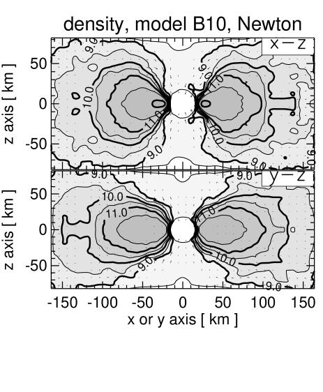
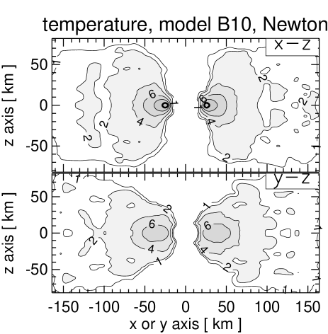
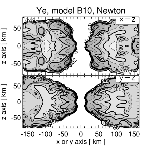
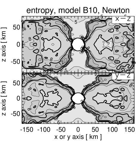
Figure 15: Vertical structure of the Newtonian Model B10 in the $x$-$z$-plane and $y$-$z$-plane near the end of the simulation ($t\approx 14.5\,$ms). The plots correspond to the cuts in the equatorial plane given in Fig. 11. The upper left figure shows contours of the baryonic mass density (measured in ${\rm g\,cm}^{-3}$) together with the flow field indicated by velocity vectors, the upper right figure displays contours of the temperature (in MeV), the lower left figure of the electron fraction $Y_{e}$, and the lower right figure of the entropy per nucleon. The density contours are spaced logarithmically with intervals of 0.5 dex (bold: $\log(\rho\left[{\rm g\,cm}^{-3}\right])=9.0,\,10.0,\,11.0,\,12.0$), the temperature contours are spaced linearly, starting with 1 MeV and 2 MeV, and then continuing in steps of 2 MeV (bold: $T=10\,{\rm MeV}$), the $Y_{e}$ contours correspond to the levels 0.02, 0.04, 0.06, 0.08, 0.10, 0.15, 0.20, 0.25, and 0.30, and the entropy levels were chosen to be 1, 2, 3, 4, 5, 6, 8, 10, 12, 14, 16, and 20 (bold: 6, 10, 20). Some of the contours are labeled with their respective values, and darker grey shading indicates higher values of a quantity.

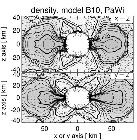
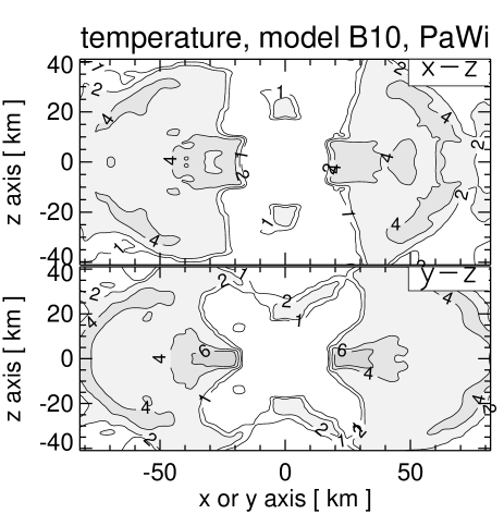
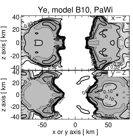
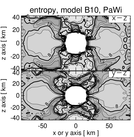
Figure 16: Vertical structure of the Paczyński-Wiita Model ${\cal B}$10 in the $x$-$z$-plane and $y$-$z$-plane near the end of the simulation ($t\approx 14.9\,$ms). The plots correspond to the cuts in the equatorial plane given in Fig. 12. The upper left figure shows contours of the baryonic mass density (measured in ${\rm g\,cm}^{-3}$) together with the flow field indicated by velocity vectors, the upper right figure displays contours of the temperature (in MeV), the lower left figure of the electron fraction $Y_{e}$, and the lower right figure of the entropy per nucleon. The density contours are spaced logarithmically with intervals of 0.25 dex (bold: $\log(\rho\left[{\rm g\,cm}^{-3}\right])=9.0,\,10.0,\,11.0$), the temperature contours are spaced linearly, starting with 1 MeV and 2 MeV, and then continuing in steps of 2 MeV (bold: $T=10\,{\rm MeV}$), the $Y_{e}$ contours correspond to the levels 0.02, 0.04, 0.06, 0.08, 0.10, 0.15, 0.20, 0.25, and 0.30, and the entropy levels were chosen to be 1, 2, 3, 4, 5, 6, 8, 10, 12, 14, 16, and 20 (bold: 6, 10, 20). Some of the contours are labeled with their respective values, and darker grey shading indicates higher values of a quantity.

Figure 17: Mass distribution in the Model B64 of Ruffert & Janka (1998b ) at $t=10\,$ms (upper figure), in the Newtonian Model B10 at time $t=14.9\,$ms (lower left figure) and in the Paczyński-Wiita Model ${\cal B}$10 at time $t=15.2\,$ms (lower right figure). In the upper panels of the figures (“z-integral”), the azimuthally averaged baryon densities were integrated along the $z$-direction from a given value of $z$ out to the grid boundary (practically infinity because of the rapidly decreasing density) and within radial intervals of width $\Delta d=1\,$km. In the lower panels (“z-d-integral”), integration in radial direction from $0$ to the value of $d$ on the abscissa was additionally performed. The baryonic mass is measured in $M_{\odot}$ and the corresponding contours of equal-mass levels are spaced logarithmically in steps of $-1$. Therefore each point $(d,z)$ in the upper panels is associated with the mass inside a hollow cylinder between $d-\Delta d$ and $d$ from $z$ to infinity, and in the lower panels with the mass inside a full cylinder between $d=0$ and $d$ from $z$ to infinity. The contours are mirrored along the $d=0$ axis in all plots and show only the mass in the volume on one side of the equatorial plane. The evacuated funnel along the system axis is clearly visible in the final stages of Models B10 and ${\cal B}$10.

4 Properties of the accretion torus

The structure of the accretion torus in the quasi-stationary state is shown in Figs. 11–22. In Figs. 11 and 12 contour plots of the density $\rho$, temperature $T$, electron fraction $Y_{e}$, and entropy per nucleon $s$ in the equatorial plane of the Newtonian Model B10 and of the Paczyński-Wiita Model ${\cal B}$10, respectively, are given at the end of the simulations. Figure 13 presents the corresponding information for the mass fractions of $\alpha$ particles and heavy nuclei in both accretion tori. In Fig. 14 the azimuthally averaged radial structure of the tori in the equatorial plane (quantities $\rho$, $T$, $Y_{e}$, and $s$) is displayed, together with the cumulative torus mass $M(d)$ as function of the equatorial radius $d$. Contour plots for $\rho$, $T$, $Y_{e}$, and $s$ in the $x$-$z$- and $y$-$z$-planes perpendicular to the equatorial plane are shown in Figs. 15 and 16. Integral mass distributions perpendicular to the equatorial plane for the initial model of our simulations as well as for the final states of Models B10 and ${\cal B}$10 are presented in Fig. 17. Finally, Figs. 21–22 give information about the azimuthal and radial velocities and the specific angular momentum of the gas in the equatorial plane of the initial model and of the evolved tori.

At the end of the simulations the tori have become nearly axially symmetric with only minor deviations (Figs. 11 and 12). Two hot spots can be seen close to the inner grid boundary at 2$R_{\rm s}$ which coincide with density maxima. They continue to carry the memory of the two very prominent spiral-like arms which are formed during the neutron star merging, grow right afterwards, and are wound up into the toroid around the black hole during the subsequent evolution. The torus of Model ${\cal B}$10 in Fig. 12 is smaller — the $\rho=10^{10}\,{\rm g\,cm}^{-3}$ contour is at 70–80 km — than the torus of Model B10 in Fig. 11 where the $\rho=10^{10}\,{\rm g\,cm}^{-3}$ contour extends out to 120–130 km. There are two reasons for that. On the one hand, the gas mass which remains around the black hole is smaller in the former model (see Table 1), on the other hand the gravitational potential is stronger in the Paczyński-Wiita case. This is the reason why despite of a difference of a factor 7 in the torus mass, both models have average densities which differ only by a factor 3 (about $3\times 10^{11}\,{\rm g\,cm}^{-3}$ for Model B10 compared to approximately $10^{11}\,{\rm g\,cm}^{-3}$ in case of Model ${\cal B}$10, see Fig. 14). The entropies in both models are nearly the same (between 5 and 10$\,k_{\rm B}$ per nucleon) and the entropy profiles are very similar in the region where most of the mass is sitting (Fig. 14). The Newtonian torus is somewhat hotter, its average temperature is around 6 MeV compared to 4 MeV for Model ${\cal B}$10. It is also more neutron rich with a mean value of $Y_{e}\approx 0.05$–0.15. Model ${\cal B}$10 has typical $Y_{e}$ values between 0.1 and 0.17 because of its lower density. This has the consequence that the neutrino opacities are smaller and thus the increase of the proton abundance by the emission of electron antineutrinos (and the cooling by the loss of neutrinos and antineutrinos of all flavors) proceeds faster. Since the hot, expanded neutron star matter radiates predominantly electron antineutrinos (see Sect. 5), the initially very neutron rich state evolves towards higher electron and proton number fractions. Due to the high temperatures, electrons are not degenerate in the tori and therefore positrons are abundant. in considerable numbers. Typical electron degeneracy parameters $\eta_{e}=\mu_{e}/T$ ($\mu_{e}$ is the electron chemical potential) are around 2, some regions have values of about 4, and in large regions one finds $\eta_{e}<2$. For the conditions in the tori, in particular due to the rather high entropies, the nucleons are mostly unbound and $\alpha$ particles and heavy nuclei are present only in small numbers. The maximum mass fractions $X_{\alpha}$ of $\alpha$ particles are around a few per cent, and heavy nuclei appear in significant abundances only where the temperature drops below 1 MeV (Fig. 13).

Figure 18: The dots represent the azimuthal velocities $v_{\varphi}(d)$ (normalized to the speed of light) of all zones in the equatorial plane of the neutron star merger Model B64 of Janka & Ruffert (1998b ) at $t=9.34\,$ms after the start of that simulation. This model was close to the one (at $t=10.0\,$ms) used as initial condition for the tori evolution simulations, Models B10 and ${\cal B}$10. The thin solid line gives the average value of the azimuthal velocities (binned in steps of 3 km), and the bold solid line the local Newtonian Kepler velocity $v_{\rm Kepler}^{\rm N}(d)$ as a function of the equatorial radius $d$.	Figure 19: Same as Fig. 21 but for the Newtonian torus Model B10 at $t=14.51\,$ms near the end of the simulation. The kinks of the curves inside the inner vacuum boundary at two Schwarzschild radii of the central black hole (about 18 km) are unphysical and caused by the interpolation of the plot data.
Figure 20: The dots represent the azimuthal velocities $v_{\varphi}(d)$ (normalized to the speed of light) of all zones in the equatorial plane of the Paczyński-Wiita torus Model ${\cal B}$10 at $t=14.94\,$ms near the end of the simulation. The thin solid line gives the average value of the azimuthal velocities and the bold solid line the local Kepler velocity $v_{\rm Kepler}^{\rm PW}(d)$ of the Paczyński-Wiita potential as a function of the equatorial radius $d$. The kinks of the curves inside the inner vacuum boundary at two Schwarzschild radii (2$R_{\rm s}$) of the central black hole (about 18 km) are unphysical and caused by the interpolation of the plot data.	Figure 21: Average specific angular momentum $j(d)=v_{\varphi}(d)d$ (in units of km times the speed of light) of the gas in the equatorial plane of the Newtonian torus Model B10 (bold solid line) at $t=14.51\,$ms and of the Paczyński-Wiita torus Model ${\cal B}$10 at $t=14.94\,$ms (thin solid line) as function of the equatorial radius $d$. The specific angular momentum $j_{\rm Kepler}^{\rm N}(d)$ corresponding to the Kepler velocity of the Newtonian gravitational potential is displayed as bold dotted line, the equivalent quantity $j_{\rm Kepler}^{\rm PW}(d)$ for the Paczyński-Wiita potential as thin dotted line. All curves start at the inner vacuum boundary at two Schwarzschild radii of the central black hole).

Figure 22: The dots give the radial velocities $v_{r}(d)$ (normalized to the speed of light) as a function of the equatorial radius $d$ for all grid zones in the equatorial plane of the Newtonian Model B10 at $t=14.51\,$ms (left) and of the Paczyński-Wiita torus Model ${\cal B}$10 at time $t=14.94\,$ms (right). The solid lines represent the mean values of all zones within binning intervals of 3 km. In the Newtonian model the velocities are very small for $d\mathrel{\vbox{\offinterlineskip\hbox{$>$}\hbox{$\sim$}}}25\,{\rm km}$ with a radial average of about $-10^{8}\,{\rm cm\,s}^{-1}$, indicating that the model has relaxed to a quasi-stationary state near the end of the simulation. In the Paczyński-Wiita torus the gas collapses rapidly inside the last stable circular orbit at $d=3R_{\rm s}\approx 27\,{\rm km}$, but expands in the region $40\,{\rm km}\mathrel{\vbox{\offinterlineskip\hbox{$<$}\hbox{$\sim$}}}d\mathrel{\vbox{\offinterlineskip\hbox{$<$}\hbox{$\sim$}}}80\,{\rm km}$ due to ongoing viscous heating and outward transport of angular momentum. Note that for $d\mathrel{\vbox{\offinterlineskip\hbox{$>$}\hbox{$\sim$}}}100\,{\rm km}$ the gas is very dilute whereas the Newtonian torus extends beyond $d=160\,{\rm km}$ (see Figs. 15 and 16). In both models the plotted values at $d\leq 20\,{\rm km}$ are not physical due to the interpolation of the data.

The perpendicular cuts (Figs. 15 and 16) confirm the nearly axially symmetric structure of the tori in Models B10 and ${\cal B}$10 at the end of the simulations. Again, some differences between the $x$-$z$- and $y$-$z$-cuts reflect the last remainders of the spiral arms which have been inflated and dissolved into the tori. While the temperature and density contours show a rather regular shape, primarily determined by the balance of pressure gradients and gravitational and centrifugal forces, the electron fraction and entropy are more irregular and patchy because both quantities carry information about the whole preceding evolution, in particular about the integral effects of neutrino emission and non-adiabatic hydrodynamic processes. Near the poles of the black hole and along the system axis, the density has decreased to values below $5\times 10^{8}\,{\rm g\,cm}^{-3}$. This is only one order of magnitude above the lower density limit which is set to $5\times 10^{7}\,{\rm g\,cm}^{-3}$ in the surroundings of the torus for numerical reasons, but nevertheless it is more than 3–4 orders of magnitude below the average densities inside the tori. In this sense we see the formation of an “evacuated”, cylindrical funnel along the rotational axis of the black hole-torus system. Material which was swept into the polar regions during and immediately after the merging of the neutron stars falls into the newly formed black hole very quickly within a free-fall time scale because it is not supported by centrifugal forces. A comparison of the initial condition for the torus simulations of Models B10 and ${\cal B}$10 (corresponding to the situation at $t\approx 10\,$ms in Model B64 of Ruffert & Janka 1998b ) with the quasi-stationary states about 5 ms later reveals this rapid cleaning of the axial funnel (see Fig. 17). In the upper panels of the three figures in Fig. 17 the contours contain all points $(d,z)$ where the cumulative gas mass $M_{\rm gas}^{\prime}(d,z)$ given by

$$M_{\rm gas}^{\prime}(d,z)\,\equiv\,\int_{z}^{\infty}{\rm d}\chi\int_{d}^{d+\Delta d}{\rm d}\xi\,\xi\int_{0}^{2\pi}{\rm d}\varphi\,\rho({\bf r})$$ (3)

is constant (the labels at the contours represent logarithmic values of the mass measured in $M_{\odot}$). The integration is done on a cylindrical grid with coordinates $(d,z,\varphi)$. The integral of Eq. (3) therefore sums up all the mass within a hollow cylinder of thickness $\Delta d=1\,$km extending from $z$ to infinity (in praxi: the upper grid boundary). The contours in Fig. 17 are mirrored along the system axis at $d=0$. Note that only the mass on one side of the equatorial plane is added up. The lower panels in Fig. 17 show the contours that correspond to constant values $M_{\rm gas}(d,z)$ according to the integral

$$M_{\rm gas}(d,z)\,\equiv\,\int_{z}^{\infty}{\rm d}\chi\int_{0}^{d}{\rm d}\xi\,\xi\int_{0}^{2\pi}{\rm d}\varphi\,\rho({\bf r})$$ (4)

which sums up the gas mass in a cylinder with radius $d$ that extends from $z$ to infinity around the system axis. The panels in Fig. 17 give detailed information about the mass distribution in the surroundings of the accretion torus. Initially, about $10^{-3}\,M_{\odot}$ of gas were distributed above the compact massive object at the center of the merger (see second panel from the top in the left column of Fig. 17). However, with increasing vertical distance $z$ from the equatorial plane the mass drops extremely rapidly already in the post-merging configuration. In the final states, the total mass inside a cylinder with radius $d\approx 15\,$km is only a few $10^{-4}\,M_{\odot}$, most of this gas is very close to the equatorial plane. Around the rotation axis the quasi-stationary states of Models B10 and ${\cal B}$10 look very similar. The larger torus mass of the Newtonian computation, however, leads to a higher mass concentration near the equatorial plane at radii $d\mathrel{\vbox{\offinterlineskip\hbox{$>$}\hbox{$\sim$}}}20\,$km. Differences are therefore visible in this region for the contours corresponding to cumulative gas masses above $10^{-5}\,M_{\odot}$. We note here that the simulations described in this paper do not include the effects of neutrino energy deposition in the vicinity of the black hole. For this reason and because we do not allow the gas densities to drop below $5\times 10^{7}\,{\rm g\,cm}^{-3}$ on the grid, our models most likely overestimate the mass of the gas surrounding the torus.

Information about the motion of the gas in the initial and final models of the torus simulations is provided by Figs. 21–22. In Fig. 21 the azimuthal velocities $v_{\varphi}(d)$ are plotted for all grid zones in the equatorial plane versus the distance $d$ from the grid center (dots) immediately before the black hole is assumed to form. The spread of the points at a given radius $d$ reflects the deviations from rotational symmetry. For an axially symmetric configuration all dots at a specific radial distance would cluster on top of each other. Also, the motion of the gas is clearly sub-Keplerian which indicates the importance of pressure support in the object. This can be seen from a comparison with the bold solid line which represents the local Newtonian Kepler velocity,

$$v_{\rm Kepler}^{\rm N}(d)=\sqrt{\frac{GM(d)}{d}}\ ,$$ (5)

given as a function of the equatorial radius $d$, with $M(d)$ being the mass enclosed by the sphere of radius $d$. The situation is different at the end of the computed torus evolution about 5 ms after the assumed formation of the black hole (Fig. 21 for the Newtonian simulation and Fig. 21 for the Paczyński-Wiita case). The spread of the dots has decreased, indicating that the torus is much more isotropic in $\varphi$ than the post-merging configuration. For distances $d\mathrel{\vbox{\offinterlineskip\hbox{$<$}\hbox{$\sim$}}}30\,$km the Newtonian torus has azimuthal velocities larger than the local Keplerian value. These allow the gas between 2$\,R_{\rm s}$ and 3$\,R_{\rm s}$ to remain on orbits around the black hole despite of a positive density and pressure gradient in this region (see Fig. 14). Also for $d>30\,$km the pressure support is important. This is suggested by the significant drop of the azimuthal velocities below the Keplerian values in Fig. 21. In the torus of Model ${\cal B}$10 the orbital velocities are much closer to the Kepler velocity for the Paczyński-Wiita potential. The value of

$$v_{\rm Kepler}^{\rm PW}(d)=\sqrt{\frac{GM(d)d}{(d-R_{\rm s})^{2}}}\ ,$$ (6)

is twice as large at $d=2R_{\rm s}$ than its Newtonian counterpart, $v_{\rm Kepler}^{\rm PW}(2R_{\rm s})=2v_{\rm Kepler}^{\rm N}(2R_{\rm s})=c$, and therefore the orbital velocities within $d\approx 50\,$km are significantly larger in Model ${\cal B}$10 than in Model B10.

The specific angular momentum $j(d)=v_{\varphi}(d)d$ of the matter in the equatorial planes of both models has typical values of $(3$–$6)\times 10^{16}\,{\rm cm^{2}\,s}^{-1}$ (Fig. 21). In the Newtonian torus the lines for $j(d)$ and the Keplerian value $j_{\rm Kepler}^{\rm N}(d)=v_{\rm Kepler}^{\rm N}(d)d$ intersect at $d\approx 30\,{\rm km}\approx 3R_{\rm s}$ which is roughly the position of the density and pressure maximum (Fig. 14). Inside this radius one has $j(d)>j_{\rm Kepler}^{\rm N}(d)$. In contrast, for the Paczyński-Wiita potential the curves of $j(d)$ and $j_{\rm Kepler}^{\rm PW}(d)=v_{\rm Kepler}^{\rm PW}(d)d$ touch at $d\approx 3R_{\rm s}$ where $j_{\rm Kepler}^{\rm PW}(d)$ has a minimum corresponding to the last stable circular orbit.

Figure 22 shows the radial velocities for all grid zones in the equatorial plane. The Newtonian Model B10 has achieved a quasi-stationary state with very small radial velocities $v_{r}$ at the end of the simulation. The average inflow velocity between 25 km and about 130 km is $\langle v_{r}\rangle\approx-10^{8}\,{\rm cm\,s}^{-1}$. At smaller distances from the black hole the gas is rapidly falling in, at distances beyond 130 km the dilute outer parts of the disk are slowly expanding due to the outward transport of angular momentum in the torus. In contrast, the Paczyński-Wiita Model ${\cal B}$10 is still evolving and has not developed stationary conditions. It expands for $40\,{\rm km}\mathrel{\vbox{\offinterlineskip\hbox{$<$}\hbox{$\sim$}}}d\mathrel{\vbox{\offinterlineskip\hbox{$<$}\hbox{$\sim$}}}80\,$km with radial velocities up to 5% of the speed of light whereas the gas interior to $d\approx 3R_{\rm s}\approx 27\,{\rm km}$ is collapsing very rapidly into the black hole, and also the dilute gas exterior to 80 km moves inward with large velocities.

Figure 23: Luminosities of electron neutrinos (labeled with e), electron antineutrinos (labeled with a), sum of all heavy-lepton neutrinos (labeled with x), and total neutrino luminosity (labeled with tot) as functions of time for the Newtonian Models B4 and B10.	Figure 24: Same as Fig. 26 but for the Paczyński-Wiita Models ${\cal B}$2 and ${\cal B}$10.
Figure 25: Average energies of the emitted electron neutrinos (labeled with nu), electron antineutrinos (anti nu), and heavy-lepton neutrinos (mu, tau) as functions of time for the Newtonian Models B4 and B10.	Figure 26: Same as Fig. 26 but for the Paczyński-Wiita Models ${\cal B}$2 and ${\cal B}$10.

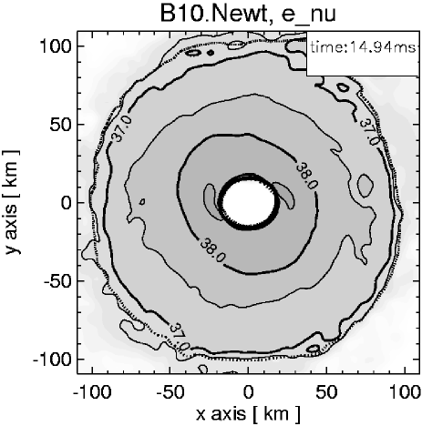
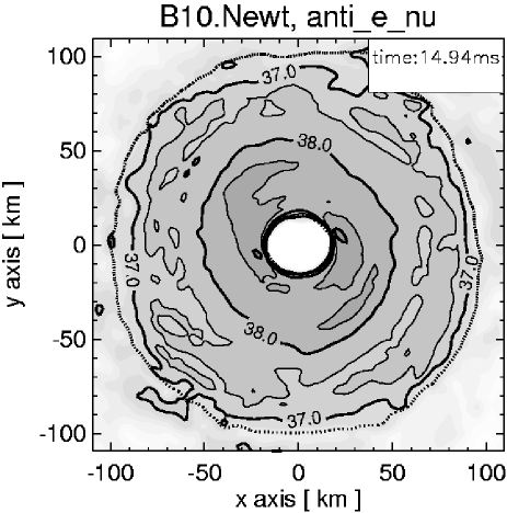
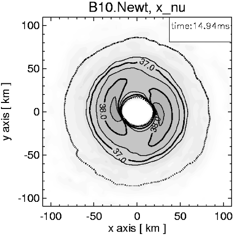
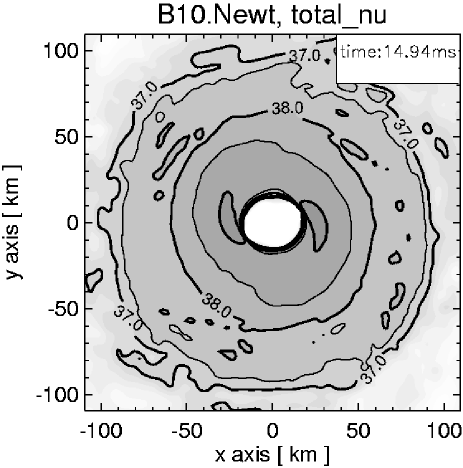
Figure 27: Surface emissivity of energy in neutrinos (measured in ${\rm erg\,cm}^{-2}{\rm s}^{-1}$) for Model B10 at the end of the simulation (time in the top right corner of the panels). The plotted contours were obtained by integration of the local energy loss rates from $z=0$ to infinity, in panel a for electron neutrinos, in panel b for electron antineutrinos, in panel c for the sum of all heavy-lepton neutrinos, and in panel d for the summed contributions from all flavors of neutrinos and antineutrinos. The contours are logarithmically spaced with intervals of 0.5 dex, bold contours are labeled with their respective values. The grey shading emphasizes the emission levels, dark grey corresponding to the strongest energy loss by neutrino emission. The dotted line marks the intersection of the $z=0$ plane with the surface of optical depth unity where neutrinos start to stream off freely.

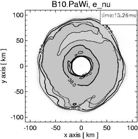
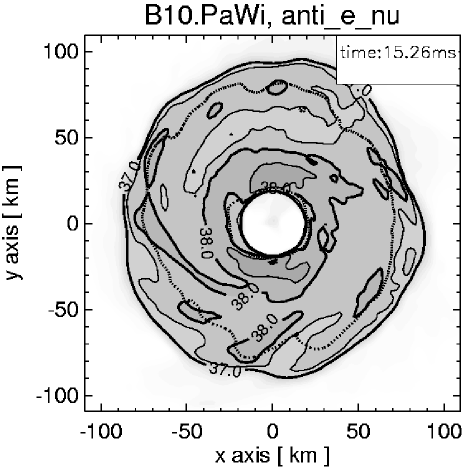
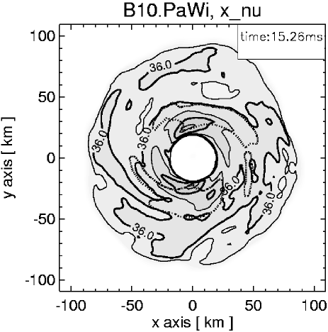
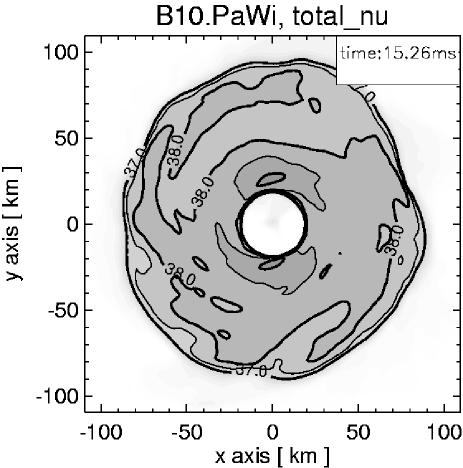
Figure 28: Same as Fig. 27 but for Model ${\cal B}$10 at time $t=15.26\,$ms.

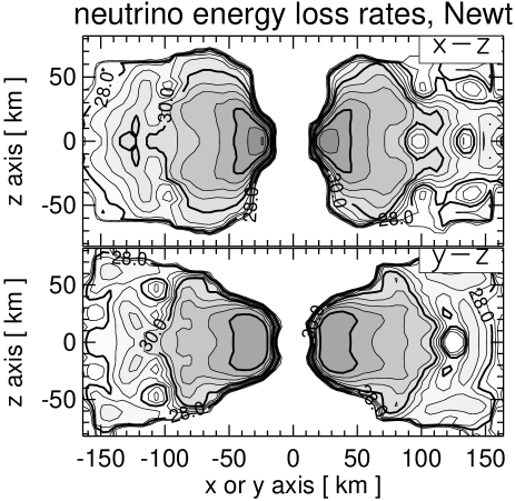
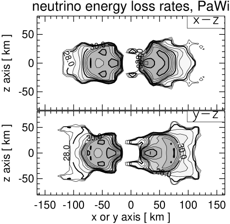
Figure 29: Contour plots of the local energy loss rates (in ${\rm erg\,cm}^{-3}{\rm s}^{-1}$ due to the emission of neutrinos and antineutrinos of all flavors. The left plot shows cuts in the $x$-$z$- and $y$-$z$-planes perpendicular to the equatorial plane of the Newtonian Model B10 near the end of the simulation, the right plot the corresponding cuts for the Paczyński-Wiita Model ${\cal B}$10. The contours are spaced logarithmically with intervals of 0.5 dex, bold contours correspond to the values 28, 30 and 32. The grey shading emphasizes the emission levels, dark grey corresponding to the strongest energy loss by neutrino emission.

5 Neutrino emission

The neutrino luminosities as functions of time for the Newtonian and Paczyński-Wiita tori are displayed in Figs. 26 and 26, respectively, and the corresponding mean energies of electron neutrinos ($\nu_{e}$), electron antineutrinos ($\bar{\nu}_{e}$) and heavy-lepton neutrinos ($\nu_{x}\equiv\nu_{\mu},\,\bar{\nu}_{\mu},\,\nu_{\tau},\,\bar{\nu}_{\tau}$) are given in Figs. 26 and 26. In order to show the sensitivity of the results to the moment the black hole is assumed to form, data from two simulations which were started at different times are plotted in each of the figures: Models B4 and B10 for the Newtonian simulations, and Models ${\cal B}$2 and ${\cal B}$10 for the Paczyński-Wiita potential.

Despite of its much smaller mass (by a factor 7.5) and lower density and temperature (see Fig. 14), the Paczyński-Wiita torus radiates neutrinos with similar luminosities and mean energies as the Newtonian model. Mainly $\nu_{e}$ and $\bar{\nu}_{e}$ are emitted. At the end of the computed evolution ($t\approx 15\,{\rm ms}$), the Newtonian model (Figs. 26 and 26) has a total luminosity $L_{\nu}=12\times 10^{52}\,{\rm erg\,s}^{-1}$, with contributions of $L_{\nu_{e}}=3.5\times 10^{52}\,{\rm erg\,s}^{-1}$ from $\nu_{e}$, $L_{\bar{\nu}_{e}}=6.5\times 10^{52}\,{\rm erg\,s}^{-1}$ from $\bar{\nu}_{e}$, and $L_{\nu_{x}}=0.4\times 10^{52}\,{\rm erg\,s}^{-1}$ from $\nu_{x}$ individually. The mean energies of the emitted neutrinos are $\langle\epsilon_{\nu_{e}}\rangle=9\,$MeV, $\langle\epsilon_{\bar{\nu}_{e}}\rangle=13\,$MeV and $\langle\epsilon_{\nu_{x}}\rangle=21\,$MeV. For the Paczyński-Wiita torus, the total luminosity reaches about 50% of the value obtained in the Newtonian simulation, $L_{\nu}=6.7\times 10^{52}\,{\rm erg\,s}^{-1}$, and the luminosities of $\nu_{e}$ and $\bar{\nu}_{e}$ reach 60–70% of the corresponding Newtonian values. The average energies of $\nu_{e}$ and $\bar{\nu}_{e}$ are slightly higher (around 10–12 MeV and 15–17 MeV, respectively). The differences between the simulations are more pronounced in case of $\nu_{x}$. At $t\approx 15\,$ms the $\nu_{x}$ luminosity is approximately one order of magnitude smaller for the Paczyński-Wiita model, and the emitted $\nu_{x}$ are less energetic with a mean energy of only 16–19 MeV instead of 21 MeV.

These differences result from the fact that the Paczyński-Wiita torus is essentially transparent for muon and tau neutrinos whereas a well defined average muon and tau neutrinosphere (to be more precise: a toriodal neutrinosurface) exists in the Newtonian model. This is clearly visible from the dotted lines in panels c of Figs. 27 and 28, which represent the intersections of the equatorial plane at $z=0$ with the neutrinosurface. The latter is defined as the two-dimensional hypersurface where the optical depth of the torus perpendicular to the equatorial plane is unity, i.e., where

$$\tau_{z,\nu_{i}}(x,y)\,\equiv\,\int_{z}^{\infty}{\rm d}z^{\prime}\,\kappa_{\nu_{i}}(x,y,z^{\prime})\,=\,1\ ,$$ (7)

with $\kappa_{\nu_{i}}(x,y,z)$ being the total opacity (defined as the inverse of the mean free path) for the energy transport of neutrino $\nu_{i}$ at a point $(x,y,z)$. In contrast, the very similar properties of the $\nu_{e}$ and $\bar{\nu}_{e}$ emission can be understood from similar thermodynamical conditions (density, temperature, entropy, see Fig. 14) at the corresponding neutrinosurfaces. The latter have an outer radius of about 100 km in case of the Newtonian torus (panels a and b in Fig. 27) and of 70–80 km in the less massive Paczyński-Wiita model (panels a and b in Fig. 28). The slightly different sizes and thus different areas of the toroidal neutrinosurfaces in panels a and b of Figs. 27 and 28 account for the moderate differences of the $\nu_{e}$ and $\bar{\nu}_{e}$ luminosities in both models.

The neutrino emission is primarily determined by the size of the neutrinosurface and the thermodynamical conditions in the layer where the average neutrino optical depth is around unity. For this reason the torus mass influences the luminosities indirectly through the radius of the neutrinosurface, until the torus mass and its density and temperature become so low that neutrino transparency is reached. The smaller torus mass and larger relative and absolute accretion rate in the Paczyński-Wiita simulation (see Figs. 5, 5 and 6) lead to a different time evolution of the neutrino luminosities (and mean neutrino energies) in both models. Extrapolation of the luminosity decrease towards the end of the simulations in Figs. 26 and 26 suggests a longer decay time scale for the Newtonian model in agreement with the longer accretion time scale given in Fig. 5.

Comparing the models with early formation of the black hole, Model B4 and Model ${\cal B}$2, with those where the black hole collapse is assumed to happen later, Models B10 and ${\cal B}$10, shows that the latter have somewhat higher neutrino luminosities. This is explained by the higher temperatures of the tori of Models B10 and ${\cal B}$10, see Fig. 8, and the correspondingly lower densities in the thermally inflated later states (Fig. 8). The effect is particularly strong for $\nu_{x}$ which are mainly produced by the annihilation of electrons and positrons into neutrino-antineutrino pairs at the conditions present in the tori, because the energy emission rate for this process is extremely temperature sensitive and increases proportional to $T^{9}$. Since the accretion rates are time dependent and the temperatures in the tori show fluctuations, the neutrino luminosities and mean energies are variable on a time scale of 1–2 ms.

The regions with the strongest neutrino emission are visible as dark grey shaded areas in Figs. 27, 28 and 29. In the former two figures the contours correspond to levels of constant energy emission rate per unit area as obtained by integration of the energy loss rate per volume from the equatorial plane at $z=0$ to infinity. In Fig. 29 vertical cuts through the Newtonian and Paczyński-Wiita accretion tori are displayed which show the total neutrino energy loss rates per unit volume in the $x$-$z$ and $y$-$z$ planes. The peak values of the emission rates are similar in both types of models but the main neutrino emitting region is less extended in case of the Paczyński-Wiita potential. The dotted lines in Figs. 27 and 28 mark the intersection of the equatorial plane with the two-dimensional hypersurface where the transport optical depth for the energy flux is unity (Eq. 7), i.e., where the spectrally averaged mean free path of the neutrinos or antineutrinos of a certain flavor is of the same order as the size of the emitting volume. Outside this neutrinosurface the neutrinos stream off essentially freely and interact by scattering or absorption with the gas particles on average only one more time. The muon and tau neutrino opacity is dominated by neutral-current scatterings off neutrons and protons. Only $\nu_{e}$ and $\bar{\nu}_{e}$ are also absorbed on neutrons and protons, respectively, via charged-current inverse beta processes. The neutrinosurface of the heavey-lepton neutrinos has a toroidal shape only in case of the Newtonian calculation (Fig. 27, panel c) but splits up into several distinct islands for the less massive and less dense Paczyński-Wiita torus which is near to neutrino-transparent conditions. The highest neutrino energy loss rates are found in a region between the inner grid boundary at $2R_{\rm s}\approx 18\,$km and an equatorial radius of approximately 70 km. In the Newtonian model significant contributions to the neutrino luminosity come even from larger distances out to about 100 km where the larger volume compensates for the smaller emission rates. The vertical cuts of Fig. 29 confirm an effect which was already visible in the density plots of Figs. 15 and 16: In the Paczyński-Wiita model, in contrast to the Newtonian simulation, gas flows towards the black hole even from the poles where it shows up by its neutrino emission in the right plot of Fig. 29.

The maximum energy loss rates of neutrinos and antineutrinos of all flavors are typically of the order $10^{32}\,{\rm erg}$ ${\rm cm}^{-3}{\rm s}^{-1}$. In single peaks values of even $10^{33}\,{\rm erg}\,{\rm cm}^{-3}{\rm s}^{-1}$ can be reached (Fig. 29). In gas with density $\rho\approx 10^{11}\,{\rm g\,cm}^{-3}$ (Figs. 15 and 16) these rates correspond to a specific energy loss of 1000$\,{\rm MeV\,s}^{-1}$ per nucleon up to even $10^{4}\,{\rm MeV}$ ${\rm s}^{-1}$ per nucleon just before the gas reaches the inner grid boundary and disappears in the black hole. For a total neutrino luminosity of $10^{53}\,{\rm erg\,s}^{-1}$ from a torus with mass of approximately 0.25$\,M_{\odot}$ in the Newtonian simulation, one calculates an average neutrino energy loss rate of 200 ${\rm MeV\,s}^{-1}$ per nucleon. This means that the binding energy of a nucleon in the gravitational potential of the 3$\,M_{\odot}$ black hole at the position of the last stable circular orbit at $3R_{\rm s}\approx 27\,$km is radiated away in less than a second, or an energy equivalent of more than 2% of the nucleon’s rest mass escapes in neutrinos within only 0.1 seconds. This estimate is in agreement with the instantaneous efficiency for the conversion of rest-mass energy into neutrino energy, $q_{\nu}\equiv L_{\nu}/(\dot{M}c^{2})$, which we calculate at the end of the simulation to be $q_{\nu}^{\rm N}\approx 1.3$% for the Newtonian torus (Table 2). In case of the Paczyński-Wiita model the corresponding value is about a factor of 2.5 lower, $q_{\nu}^{\rm PW}\approx 0.5$%. These numbers are significantly smaller than the maximum efficiency of 5.7% for relativistic disk accretion onto a Schwarzschild black hole (8.3% for a thin Newtonian accretion disk) because the tori are not transparent for neutrinos. Due to the high densities and temperatures, the diffusion time scale for neutrinos becomes longer than the accretion time scale of the gas into the black hole. Therefore the tori are advection dominated and cooling does not reach its maximum possible efficiency.

Table 2: Torus mass $M_{\rm v}$, black hole mass accretion rate $\dot{M}_{\rm v}$, typical accretion time scale of the torus, $t_{\rm acc}\equiv M_{\rm v}/\dot{M}_{\rm v}$, total neutrino luminosity $L_{\nu}$, efficiency $q_{\nu}\equiv L_{\nu}/(\dot{M}c^{2})$, integral rate of energy deposition by neutrino-antineutrino annihilation around the accretion torus, $\dot{E}_{\nu\bar{\nu}}$, and efficiency $q_{\nu\bar{\nu}}\equiv\dot{E}_{\nu\bar{\nu}}/L_{\nu}$ for the Newtonian Model B10 and Paczyński-Wiita Model ${\cal B}$10. All quantities are given at the time $t_{\rm fin}$ when the simulation was stopped. $E_{\nu\bar{\nu}}$ gives the estimated total energy deposition by $\nu\bar{\nu}$ annihilation in the time interval $t_{\rm fin}+t_{\rm acc}$ which is roughly equal to the duration of neutrino emission.

model	potential	$t_{\rm fin}$	$M_{\rm v}$	$\dot{M}_{\rm v}$	$t_{\rm acc}$	$L_{\nu}$	$q_{\nu}$	$\dot{E}_{\nu\bar{\nu}}$	$q_{\nu\bar{\nu}}$	$E_{\nu\bar{\nu}}$
		ms	$10^{-2}M_{\odot}$	$M_{\odot}\,{\rm s}^{-1}$	ms	$10^{52}\frac{\rm erg}{\rm s}$		$10^{50}\frac{\rm erg}{\rm s}$		$10^{49}{\rm erg}$
B10	Newt	14.9	26.4	5.	53.	12.	0.013	4.9	0.0041	3.3
${\cal B}$10	PaWi	15.2	3.5	7.	5.	6.7	0.005	3.1	0.0046	0.6

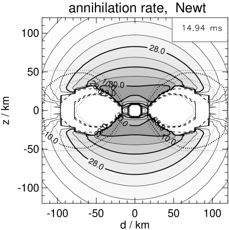
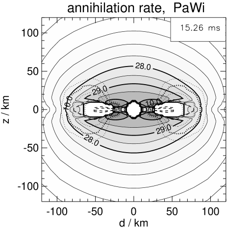
Figure 30: Maps of the local energy deposition rates (in erg cm${}^{-3}\,$s^-1) by $\nu\bar{\nu}$ annihilation into $e^{+}e^{-}$ pairs in the surroundings of the accretion torus of the Newtonian Model B10 at time $t=14.94\,$ms (left) and of the Paczyński-Wiita Model ${\cal B}$10 at time $t=15.26\,$ms (right). The values shown as solid contour lines in a plane perpendicular to the equatorial plane were obtained as averages over the azimuthal angle around the $z$-axis. The abscissa $d$ measures the distance from the grid center in the $x$-$y$-plane. The white octagonal area around the center with a semidiameter of one Schwarzschild radius indicates the presence of the central black hole. The contours are logarithmically spaced in steps of 0.5 dex, the grey shading emphasizes the levels with dark grey meaning high energy deposition rate. The energy deposition rate was evaluated only in that region around the torus where the baryon mass density is below $10^{11}\,{\rm g\,cm}^{-3}$. The integral value of the energy deposition rate at the displayed time is $4.9\times 10^{50}\,{\rm erg\,s}^{-1}$ for Model B10 (left) and $3.1\times 10^{50}\,{\rm erg\,s}^{-1}$ for Model ${\cal B}$10 (right). The dashed lines mark the (approximate) positions of the neutrino“spheres” of $\nu_{e}$, $\bar{\nu}_{e}$, and $\nu_{x}$ (from outside inward), defined by the requirement that the optical depths in $z$-direction are $\tau_{z,\nu_{i}}=1$ (see also Eq. (7) and Figs. 27 and 28). The dotted contour lines represent levels of constant values of the azimuthally averaged mass density, also logarithmically spaced with intervals of 0.5 dex, the bold dotted line corresponding to $\rho=10^{10}\,{\rm g\,cm}^{-3}$.

6 Neutrino-antineutrino annihilation

We evaluate our hydrodynamical models in a post-processing step for the annihilation of neutrinos and antineutrinos into electron-positron pairs. The corresponding methods were explained in detail in Ruffert & Janka (1998a ) and in Ruffert et al. (ruf97 (1997)). Neutrinos and antineutrinos emitted from the hot accretion torus interact with each other in the surroundings with a finite probability which depends on the number densities and energies of these neutrinos and on the angle between the directions of neutrino and antineutrino propagation (see Goodman et al. goo87 (1987), Cooperstein et al. coo87 (1987), Mayle may90 (1990); also Ruffert et al. ruf97 (1997)). Therefore the local energy deposition rate by $\nu\bar{\nu}$ annihilation increases proportional to the product of neutrino and antineutrino luminosities and the spectrally averaged neutrino energy, times a factor that accounts for the dependence on the angular distribution of the neutrinos. The annihilation rate drops rapidly with increasing distance from the neutrino source because both the neutrino number densities and the mean angle of neutrino-antineutrino collisions decrease.

The computational procedure to obtain the energy deposition outside the accretion torus can be briefly summarized as follows. In a first step the hydrodynamical model at a chosen time is mapped from the nested grids of the simulation onto an equidistant cartesian grid. Next, for each type of neutrino or antineutrino the two-dimensional surface is determined where the optical depth in $z$-direction is unity (see Eq. 7). The neutrino energy loss rates from the torus volume are projected onto these surfaces and treated as surface emissivities. In order to compute the energy deposition rate per unit volume by $\nu\bar{\nu}$ annihilation at a point $\@vec{r}$, one has to sum up the contributions by the neutrino and antineutrino emission from all parts of the neutrinosurfaces which radiate into the direction of point $\@vec{r}$. The total energy deposition rate includes contributions from all three flavors of neutrinos and antineutrinos. Finally, volume integrals of the energy deposition rate can be obtained by summation over specified regions of the equidistant cartesian grid. The results of this evaluation are plotted in Figs. 30 and 31 for the final states of our torus simulations. The figures show azimuthally averaged (around the $z$-axis) quantities in a plane perpendicular to the equatorial plane.

Figure 30 displays contours of constant energy deposition rate per unit volume in those regions around the Newtonian (left) and Paczyński-Wiita (right) tori where the baryonic mass density is less than $10^{11}\,{\rm g\,cm}^{-3}$. The dotted lines represent density contours, the dashed lines mark the positions of the average neutrinosurfaces of $\nu_{e}$, $\bar{\nu}_{e}$ and $\nu_{x}$ (from outside outward). The $\nu_{e}$ neutrinosurface is very close to the toroidal surface which corresponds to a density of $\rho=10^{11}\,{\rm g\,cm}^{-3}$. The neutrinosurfaces of $\bar{\nu}_{e}$ and $\nu_{x}$ are deeper inside, because $\bar{\nu}_{e}$ are absorbed onto protons which are less abundant in the torus than neutrons, and the streaming of the $\nu_{x}$ is inhibited only by neutral-current scatterings off nucleons. Both the dashed and dotted sets of contours demonstrate that the Paczyński-Wiita torus is significantly smaller and nearly transparent for electron antineutrinos and heavy-lepton neutrinos.

Figure 31: Cumulative energy deposition rates by $\nu\bar{\nu}$ annihilation for the Newtonian Model B10 at time $t=14.9\,$ms (upper panel) and for the Paczyński-Wiita Model ${\cal B}$10 at time $t=15.2\,$ms (lower panel). The azimuthally averaged annihilation rate per unit volume was integrated along the $z$-direction from a given value of $z$ out to the grid boundary (practically infinity because of the rapid decrease of the annihilation rate with distance) and in addition from $d=0$ to the value of $d$ given on the abscissa. The contours are spaced logarithmically in steps of 0.5 dex and represent values only for the hemisphere above the equatorial plane (measured in erg s^-1). They are mirrored along the $z$-axis. The two panels should be compared with the lower panels in Fig. 17 and were constructed in an analogous way.

The maximum energy deposition rates by $\nu\bar{\nu}$ annihilation (solid contours in Figure 30) exceed $10^{30}\,{\rm erg\,cm}^{-3}{\rm s}^{-1}$ in the polar regions above and below the equatorial plane at heights $|z|$ between 10 km and 30 km in the Newtonian model. Such high values occur also in the Paczyński-Wiita simulation, but only very close to the surface of the torus and to the equatorial plane, between the black hole and the last stable circular orbit at $3R_{\rm s}\approx 27\,$km. the values at larger distances $|z|$ are typically one order of magnitude lower than in the Newtonian model at the same $|z|$. Within the displayed region, the energy deposition rate along the polar axis decreases roughly proportional to $z^{-6}$ for $|z|\mathrel{\vbox{\offinterlineskip\hbox{$>$}\hbox{$\sim$}}}30\,$km.

The integral rate of heating by $\nu\bar{\nu}$ annihilation in the computed volume is $4.9\times 10^{50}\,{\rm erg\,s}^{-1}$ for the Newtonian model. About 40% of this energy ($1.9\times 10^{50}\,{\rm erg\,s}^{-1}$) are deposited in a cylinder with radius $3R_{\rm s}=27\,$km around the $z$-axis, 90% ($4.4\times 10^{50}\,{\rm erg\,s}^{-1}$) in a cone with opening half-angle of 30–40 degrees which is approximately bounded by the isodensity contour for $\rho=10^{10}\,{\rm g\,cm}^{-3}$ in Fig. 30. The corresponding numbers for the Paczyński-Wiita torus are $3.1\times 10^{50}\,{\rm erg\,s}^{-1}$ for the total energy deposition, of which $1.3\times 10^{50}\,{\rm erg\,s}^{-1}$ end up in the cylinder along the axis and $1.9\times 10^{50}\,{\rm erg\,s}^{-1}$ in the cone. From these values one computes the total conversion efficiencies $q_{\nu\bar{\nu}}\equiv\dot{E}_{\nu\bar{\nu}}/L_{\nu}$ of neutrino energy into energy of the pair-plasma fireball to be $q_{\nu\bar{\nu}}^{\rm N}=4.1\times 10^{-3}$ and $q_{\nu\bar{\nu}}^{\rm PW}=4.6\times 10^{-3}$ (Table 2).

Figure 31 provides information about the spatial distribution of the cumulative energy deposition rates in both models. The plots show $z$-$d$-integrals of the rates per unit volume, $\dot{Q}_{\nu\bar{\nu}}({\bf r})$, which are computed as

$$\dot{E}_{\nu\bar{\nu}}(d,z)\,\equiv\,\int_{z}^{\infty}{\rm d}\chi\int_{0}^{d}{\rm d}\xi\,\xi\int_{0}^{2\pi}{\rm d}\varphi\,\dot{Q}_{\nu\bar{\nu}}({\bf r})\ .$$ (8)

These plots are thus constructed in analogy to the panels of the $z$-$d$ integrals for the mass in Fig. 17. Note that the values correspond to the energy that is deposited only on one side of the equatorial plane. A large part of the energy, nearly $10^{50}\,{\rm erg\,s}^{-1}$, is dumped within 30 km around the polar axis and at heights larger than about $30\,$km above (and below) the equatorial plane in the Newtonian model and at heights larger than about $10\,$km in the Paczyński-Wiita case. According to Fig. 17 there are less than $10^{-4}\,M_{\odot}$ of gas in these regions in both models. A comparison of the two panels in Fig. 31 reveals that in the Paczyński-Wiita simulation the energy is more concentrated towards the equatorial plane so that at heights $|z|\mathrel{\vbox{\offinterlineskip\hbox{$>$}\hbox{$\sim$}}}30\,$km the numbers are about one order of magnitude lower than in the Newtonian model. This difference is explained mainly by the smaller size of the neutrinospheres in the less massive Paczyński-Wiita torus. A minor part of the effect is also due to the lower neutrino luminosities which reach only little more than half the values of the Newtonian model.

7 Analytical estimates

7.1 Viscosity and evolution

The evolution of the Newtonian torus on longer time scales will be governed by the outward-directed viscous transport of angular momentum. Since the Euler equations which are solved numerically with the PPM method do not contain viscosity terms, and since this scheme does not require any artificial viscosity to treat shock waves, the most important viscous dissipation in the absence of shocks comes from the numerical viscosity of the code. The latter is associated with the discretization of the equations and thus depends on the chosen grid resolution, but is also determined by the input physics implemented in the hydrodynamics code. In case of the quasi-stationary Newtonian Model B10 we shall estimate the size of this numerical viscosity from the torus properties.

With the average value of the radial inflow velocity, $\langle v_{r}\rangle\approx-10^{8}\,{\rm cm\,s}^{-1}$ (see Fig. 22 and Sect. 4), and a mean radius $\langle d\rangle$ of about 50 km we estimate an accretion time scale of $t_{\rm acc}=\langle d\rangle/\langle v_{r}\rangle\approx 50\,$ms in very good agreement with the independent determination via the mass accretion rate of the black hole, $t_{\rm acc}=M_{\rm v}/\dot{M}_{\rm v}\approx 53\,$ms (see Fig. 5 and Table 2). The viscous time scale is given by $t_{\rm vis}\approx M_{\rm v}/(6\pi\eta R_{\rm s})$ — see Eq. (13) in Ruffert et al. (ruf97 (1997)) — with the dynamic viscosity $\eta\sim\alpha(\rho Hv_{\rm Kepler})$ where $H\sim R_{\rm s}$ is the height of the torus, $\rho$ the average density in the torus, $v_{\rm Kepler}=\Omega_{\rm Kepler}(d)d=\sqrt{GM_{\rm BH}/d}$ the Keplerian velocity at a representative radius $d\sim 4R_{\rm s}$, and $\alpha$ the dimensionless $\alpha$-viscosity parameter. Using $\rho=M_{\rm v}/V_{\rm t}$ with the torus volume $V_{\rm t}\sim 2\pi^{2}R_{\rm s}^{2}d$, one finds $\alpha\sim\left[\Omega_{\rm Kepler}(d)t_{\rm vis}\right]^{-1}$. Setting $t_{\rm vis}=t_{\rm acc}=\langle d\rangle/\langle v_{r}\rangle$ we get a value for the $\alpha$-parameter associated with the numerical viscosity of $\alpha\sim\langle v_{r}\rangle/v_{\rm Kepler}(d)\sim 0.01$. It is interesting to note that the torus shapes computed by Popham & Gammie (pop98a (1998)) for such values of the $\alpha$-viscosity look very similar to the cross sections through the tori of our simulations plotted in Figs. 15, 16 and 30.

The numerical viscosity in our simulations therefore corresponds to a value $\alpha\sim 0.01$, which is a bit higher than the “optimum” value $\alpha^{\ast}=\eta^{\ast}/(\rho Hv_{\rm Kepler})$ where the viscous energy dissipation and the energy emission by neutrinos are balanced, a requirement which ensures maximum efficiency for the conversion of rest-mass energy into neutrinos. Ruffert et al. (ruf97 (1997)) estimated $\alpha^{\ast}\sim(1.7\,...\,6.6)\times 10^{-3}(R_{\rm s}/9\,{\rm km})^{7/2}(M_{\rm v}/0.1\,M_{\odot})^{-3/2}$ on grounds of a very simple one-zone model of the torus. Consistent with the larger value of the viscosity, the mass accretion rate of the black hole was found to be $\dot{M}_{\rm v}\approx 5\,M_{\odot}\,{\rm s}^{-1}$ in the numerical simulation (Fig. 5 and Table 2), which is somewhat higher — and the corresponding lifetime $t_{\rm acc}$ of the torus somewhat shorter — than estimated by Ruffert et al. (ruf97 (1997)) for the optimum value $\alpha^{\ast}$. This implies that the torus does not lose energy in neutrinos at the maximum theoretical efficiency of about 8.3% for disk accretion on a nonrotating black hole in Newtonian gravity. I.e., the torus in the numerical simulation is advection dominated, in agreement with the findings in Sect. 5 (see also Table 2). Because of the high densities and temperatures in the torus, the matter is not transparent to neutrinos and the neutrino diffusion time is longer than the accretion time of the gas. Therefore a sizable fraction of the gravitational binding energy that is dissipated into heat is carried into the black hole before neutrinos are able to transport it away. Although the neutrino luminosities obtained in the numerical simulations are close to those estimated by Ruffert et al. (ruf97 (1997)), the shorter lifetime of the torus leads to a smaller time integral of the radiated energy.

Popham et al. (pop98b (1998)) have calculated self-consistent stationary models for neutrino emitting accretion disks of black holes for a wide range of parameters. With the large accretion rates and high densities, the tori obtained in our simulations are in an extreme corner of their parameter space where the idealized treatment of the neutrino cooling by Popham et al. (pop98b (1998)), who essentially assumed neutrino-transparent conditions, reaches its limits of applicability.

Finally, we point out that neutrino emission is rather inefficient in transporting away angular momentum and therefore this is not the driving force of the torus evolution in our investigated cases. Setting the mass accretion rate by the black hole in relation to the angular momentum loss rate, $\dot{J}\sim\dot{M}_{\rm v}\Omega_{\rm Kepler}d^{2}$, and requiring $\dot{J}$ to be equal to the angular momentum carried off by neutrinos, $\dot{J}=\dot{J}_{\nu}\sim(L_{\nu}/c^{2})\Omega_{\rm Kepler}d^{2}$, one finds $\dot{M}_{\rm v}\sim L_{\nu}/c^{2}$. For a neutrino luminosity of $L_{\nu}=10^{53}\,{\rm erg}\,{\rm s}^{-1}$ this gives a mass accretion rate of the order of $\dot{M}_{\rm v}\sim{1\over 20}M_{\odot}\,{\rm s}^{-1}$ which is two orders of magnitude below our numerically determined numbers.

Figure 32: Geodesics of (massless) neutrinos emitted tangentially from a toroidal accretion disk (white circle) with assumed semidiameter $R_{\rm t}$ of one Schwarzschild radius, $R_{\rm s}=9\,$km, (left) and of three Schwarzschild radii (right) in the vicinity of a black hole (black circle) with a mass of $3M_{\odot}$. The torus center is at $x=3R_{\rm s}+R_{\rm t}$, the black circle has a radius of $1R_{\rm s}$.

Table 3: In the second and third column ratios of general relativistic (“GR”) to Newtonian (“N”) results are given for the integral energy deposited by $\nu\bar{\nu}$ annihilation for the different values of $\alpha\equiv R_{\rm t}/R_{\rm s}$ listed in the first column. The other columns contain values of the factor ${\cal U}/(\alpha\beta{\cal V})$ in Eq. (21). This factor decides about the importance of neutrino-electron and neutrino-positron scattering relative to $\nu\bar{\nu}$ annihilation. It is assumed that the neutrinos are emitted from a toroidal neutrinosurface with radius $R_{\rm t}$ and center at $3R_{\rm s}+R_{\rm t}$. The energy deposition rates by annihilation or scattering are integrated either over the volume of a cylinder with radius $3R_{\rm s}$ around the system axis, or over the volume of a cone enclosed by the rotated boundary curve of Eq. (10), respectively.

	$\nu\bar{\nu}$	$\nu\bar{\nu}$	$e\nu$	$e\nu$	$e\nu$	$e\nu$
$R_{\rm t}/R_{\rm s}$	GR/N	GR/N	N	GR	N	GR
	cylinder	cone	cylinder	cylinder	cone	cone
0.5	0.67	0.84	0.124	0.083	0.115	0.074
1.0	0.68	0.85	0.097	0.069	0.089	0.061
2.0	0.72	0.89	0.064	0.049	0.057	0.043
3.0	0.75	0.92	0.045	0.037	0.040	0.032
4.0	0.77	0.94	0.033	0.028	0.029	0.024

7.2 General relativistic effects

The torus simulations described in this paper were performed with basically Newtonian physics except that the gravitational potential was replaced by a Paczyński-Wiita potential in some cases. Also the emission of gravitational waves and the corresponding back-reaction on the hydrodynamic flow were included, which, however, is not important for the nearly axially symmetric black hole-torus configurations.

The influence of general relativistic effects on the neutrino emission and on the neutrino-antineutrino annihilation are not obvious because of several competing effects which partly cancel each other (see, e.g., Shapiro & Teukolsky sha83 (1983), Luminet lum79 (1979), Marck mar96 (1996), Cardall & Fuller car97 (1997), Usui et al. usu98 (1998)). The effects considered here are :

(1) General relativistic blueshifting of those neutrinos which are emitted from the accretion torus in the direction of the black hole before they annihilate, and redshifting of those neutrinos which annihilate at distances from the black hole larger than the radius of their production.

(2) Gravitational redshifting of the energy as the electron-positron pair plasma expands away from the site of its creation by $\nu\bar{\nu}$ annihilation.

(3) General relativistic ray bending of the neutrino trajectories which changes the average angles at which neutrinos and antineutrinos collide and thus also changes the rate of $\nu\bar{\nu}$ annihilation.

(4) Gravitational trapping of the energy which is deposited in the close vicinity of the event horizon by $\nu\bar{\nu}$ annihilation and therefore is not able to escape from the strong gravitational attraction of the black hole but is ultimately sucked in by the hole.

It is not easy to implement these effects consistently into the hydrodynamic simulations and into the post-processing procedure which we used to evaluate our models for neutrino-antineutrino annihilation. In order to estimate the relative changes due to general relativity approximately, we therefore consider a simplified treatment for an idealized model geometry which mimics sufficiently closely the situation described by the hydrodynamic results. For this purpose, we assumed that the neutrinos are emitted from a neutrinosurface that has the shape of a torus centered on the equatorial plane. At least in case of the Newtonian accretion disk, which is optically thick for neutrinos, Fig. 30 shows that this picture is indeed appropriate. In the following analysis we shall explicitly presume that the black hole-torus configuration is axially symmetric. We neglect effects due to the relativistic Doppler shift of the neutrinos emitted from the torus although the gas orbits around the black hole at a fair fraction of the speed of light.

Integrating the energy deposition rate by $\nu\bar{\nu}$ annihilation over a volume $V$ outside of the torus, one can write

$$\dot{E}_{\nu\bar{\nu}}\,=\,\int_{V}{\rm d}^{3}{\bf r}\,\dot{Q}_{\nu\bar{\nu}}({\bf r})\,\equiv\,R_{\rm s}^{-1}\cdot{\cal R}\,{\cal L}\,{\cal V}\,,$$ (9)

where ${\cal R}=9R_{\rm s}^{4}R_{\rm t}^{-2}(3R_{\rm s}+R_{\rm t})^{-2}$ is a dimensionless factor that depends on the torus radius $R_{\rm t}$, the horizon radius of the black hole, $R_{\rm s}$, and the radius of the torus center, $3R_{\rm s}+R_{\rm t}$. The factor ${\cal L}$ contains the weak interaction coefficients $c_{\nu_{i}\bar{\nu}_{i}}$ ($i=e,\mu,\tau$) and is proportional to the product of the neutrino and antineutrino luminosities multiplied by the sum of the average neutrino and antineutrino energies which determine the $\nu\bar{\nu}$ annihilation rate, i.e., ${\cal L}\propto\sum_{i}c_{\nu_{i}\bar{\nu}_{i}}L_{\nu_{i}}L_{\bar{\nu}_{i}}(\langle\epsilon_{\nu_{i}}\rangle+\langle\epsilon_{\bar{\nu}_{i}}\rangle)$. The term ${\cal V}$ is also a dimensionless factor that results from the volume integral and carries information about the angular distributions of the neutrinos and antineutrinos at the positions ${\bf r}$.

Two different axially symmetric volumes are considered. On the one hand, the integration is performed over a cylinder with radius $3R_{\rm s}$ around the symmetry axis of the torus-black hole system. On the other hand, the volume of a cone is considered whose surface is described by a rotation of the curve

$${z\over 3R_{\rm s}}\,=\,\pm\,{x\over 3R_{\rm s}}\,\sqrt{\left({x\over 3R_{\rm s}}\right)^{\!2/3}-1}\quad\ {\rm for}\ \,{x\over 3R_{\rm s}}\,\geq\,1$$ (10)

around the symmetry axis. In all points on this surface the component of the gravitational force parallel to the equatorial plane is balanced by the centrifugal force of matter which has angular momentum equal to the Keplerian value at radius $3R_{\rm s}$, $j=j_{\rm Kepler}(3R_{\rm s})=\sqrt{6}GM_{\rm BH}/c$. This surface may approximate the boundary of a baryon-free funnel along the axis.

If one assumes that the value of the integrand on the axis at vertical height $z$ is representative of all values in the plane defined by this $z$, one can make use of the axial symmetry which allows one to calculate the $\nu\bar{\nu}$ annihilation rate along the axis particularly easily. The integrations parallel and vertical to the system axis can then be separated, and only a one-dimensional integral for ${\cal V}$ is left for numerical evaluation :

$${\cal V}\,=\,\int_{\xi_{\rm min}}^{\infty}{\rm d}\xi\,W(\xi)\,.$$ (11)

First we consider the cases without general relativistic effects. For the cylindrical volume one sets $\xi\equiv z/R_{\rm s}$ and starts the integration at $z=R_{\rm s}$, i.e. $\xi_{\rm min}=1$. The integrand is found to be

$$W(\xi) \equiv W_{\rm cyl}^{\rm N}(\xi)\,=\,$$ (12)

$$= (\mu_{1}-\mu_{0})^{2}\times\biggl{[}{3\over 2}+{1\over 6}\left(\mu_{1}^{2}+\mu_{1}\mu_{0}+\mu_{0}^{2}\right)^{2}$$

$$- {1\over 2}\left(\mu_{1}+\mu_{0}\right)^{2}-{1\over 3}\left(\mu_{1}^{2}+\mu_{1}\mu_{0}+\mu_{0}^{2}\right)\biggr{]}$$

with

$$\mu_{0,1}\,=\,\mu_{0,1}(\xi)\,=\,{\xi\sqrt{\beta^{2}+\xi^{2}-\alpha^{2}}\mp\alpha\beta\over\beta^{2}+\xi^{2}}$$ (13)

where $\alpha\equiv R_{\rm t}/R_{\rm s}$ and $\beta\equiv 3+\alpha$. The minus sign in Eq. (13) corresponds to $\mu_{0}=\cos\theta_{0}$, the plus sign to $\mu_{1}=\cos\theta_{1}$, if $\theta_{0}>\theta_{1}$ and $\theta_{0}$ and $\theta_{1}$ are the angles between the symmetry axis and the direction of rays that leave the torus surface tangentially and go to an observer on the axis. Taking the variable of integration to be $\xi\equiv x/(3R_{\rm s})$, one can derive in case of the conical volume :

$$W(\xi) \equiv W_{\rm con}^{\rm N}(\xi)\,=\,$$ (14)

$$= \xi^{2}\,{4\xi^{2/3}-3\over\sqrt{x^{2/3}-1}}\,W_{\rm cyl}^{\rm N}(3\xi\sqrt{\xi^{2/3}-1})\,,$$

where the expression in backets is the argument with which $W_{\rm cyl}^{\rm N}$ of Eq. (12) has to be evaluated. The lower integral boundary is now given by the value $\xi_{\rm min}$ for which the relation $\xi\sqrt{\xi^{2/3}-1}=1/3$ is fulfilled.

The relativistic effects listed above can be taken into account in the following approximate way. General relativistic ray bending (point (3) in the list at the beginning of this section) requires to replace the Euclidian values of $\mu_{0}$ and $\mu_{1}$ of Eq. (13) by their relativistic counterparts. These are found by tracing geodesics from an observer position on the axis to the points where they hit the torus surface tangentially. Figure 32 shows two examples where we calculated the ray trajectories in the gravitational field of a black hole with approximately $3M_{\odot}$ for a torus with radius $R_{\rm t}=1R_{\rm s}$ and a torus with radius $R_{\rm t}=3R_{\rm s}$, respectively. In our analysis we allow for only one torus image and thus neglect that neutrino trajectories may be bent around the black hole to cross the system axis more than once. Blueshift, redshift and radiation trapping (points (1), (2) and (4), respectively) are accounted for by assuming that they can be split off in a separate factor $\langle S^{\rm GR}C^{\rm GR}\rangle$ in the integrand of Eq. (11). Thus for the cylindrical integration volume we take

$$W(\xi)\,\equiv\,W_{\rm cyl}^{\rm GR}(\xi)\,=\,W_{\rm cyl}^{\rm N}(\xi)\,\langle S^{\rm GR}\cdot C^{\rm GR}\rangle(\xi)\,,$$ (15)

and for the integration over the cone we use

$$W(\xi) \equiv W_{\rm con}^{\rm GR}(\xi)\,=\,$$ (16)

$$= W_{\rm con}^{\rm N}(\xi)\,\langle S^{\rm GR}\cdot C^{\rm GR}\rangle(3\xi\sqrt{\xi^{2/3}-1})\,.$$

The factor $\langle S^{\rm GR}C^{\rm GR}\rangle$ in Eq. (15) depends on $\xi$ and in Eq. (16) on $3\xi\sqrt{\xi^{2/3}-1}$, and the brackets $\langle...\rangle$ indicate that the product $S^{\rm GR}C^{\rm GR}$ has been averaged over the plane at constant $z$. For the latter averaging procedure one has to notice that $S^{\rm GR}C^{\rm GR}$, as specified below, has a weakly diverging singularity at the event horizon, but its integral has a finite value and is regular.

The red- and blueshift factor $S^{\rm GR}$ can be approximated by

$$S^{\rm GR}(r) = {\rm e}^{2\phi(r_{\rm o})}\,\left({{\rm e}^{\phi(r_{\rm o})}\over{\rm e}^{\phi(r)}}\right)^{\!3}$$ (17)

$$\approx \left(1-{R_{\rm s}\over 3R_{\rm s}+R_{\rm t}}\right)^{\!5/2}\left(1-{R_{\rm s}\over r}\right)^{\!-3/2}$$

where $r$ denotes the radius where neutrinos and antineutrinos annihilate, the lapse function is given by ${\rm e}^{\phi(r)}=\sqrt{1-R_{\rm s}/r}$, and the second expression is obtained by taking $r_{\rm o}\approx 3R_{\rm s}+R_{\rm t}$ as the mean radius from where neutrinos and antineutrinos originate. The first factor ${\rm e}^{2\phi(r_{\rm o})}$ in Eq. (17) accounts for the redshift and time dilation from $r_{\rm o}$ to infinity, and the second factor $({\rm e}^{\phi(r_{\rm o})}/{\rm e}^{\phi(r)})^{3}$ for the blueshift or redshift between $r_{\rm o}$ and $r$.

Close to the event horizon only photons moving nearly radially outward can escape from the gravitational attraction of the black hole whereas photons propagating with large angles relative to the outward direction are captured by the hole. We assume that the electron-positron-photon plasma is locally isotropic and neglect hydrodynamic effects. This allows us to estimate the escape probability of energy produced by $\nu\bar{\nu}$ annihilation at radius $r$ from the fraction of photons on escape trajectories according to (Shapiro & Teukolsky sha83 (1983)) :

$$C^{\rm GR}(r)\,\approx\,{1\over 2}\,\left[1\pm\sqrt{1-{27\over 4}\left({R_{\rm s}\over r}\right)^{\!2}\left(1-{R_{\rm s}\over r}\right)}\,\,\right]\,,$$ (18)

with the minus sign holding for $R_{\rm s}\leq r\leq{3\over 2}R_{\rm s}$ and the plus sign for $r>{3\over 2}R_{\rm s}$. At $r={3\over 2}R_{\rm s}$ a fraction of 50% of the pair plasma is able to escape to infinity. The assumption of local isotropy probably implies an underestimation of the escape probability because the non-zero radial momentum of $e^{\pm}$ pairs produced by $\nu\bar{\nu}$ annihilation is not taken into account. Ray bending towards the black hole and positive pressure gradients, on the other hand, act in the opposite direction and reduce the expansion of the pair plasma out of the close vicinity of the event horizon. Therefore we consider Eq. (18) as a reasonable zeroth-order estimate.

The expressions of Eqs. (17) and (18) are now inserted into Eqs. (15) and (16) to evaluate the integral of Eq. (11). Equation (9) then yields the energy deposition rate by $\nu\bar{\nu}$ annihilation as measured by an observer at rest at infinity, when the neutrino luminosities and the mean neutrino energies are taken as measured at the neutrino source. The annihilation luminosities including general relativistic corrections are reduced relative to the Newtonian results. The calculated reduction factors are listed in Table 3 for different values of the parameter $R_{\rm t}/R_{\rm s}$. Relativistic effects decrease the available energy in all investigated cases by typically 10–30%, mainly because of redshift to infinity and radiation capture by the black hole. However, these two effects are nearly compensated by the increase of the $\nu\bar{\nu}$ annihilation probability due to the facts that the neutrinos emitted towards the black hole are blueshifted and the $\nu\bar{\nu}$ annihilation rate rises with the square of the neutrino luminosity times the average neutrino energy. It is interesting to note that general relativistic ray bending reduces the angle under which the torus surface is seen from a position on the system axis near the black hole, whereas the viewing angle of the torus is increased relative to the Euclidean angle at large distances. For this reason, ray bending implies a reduction of the $\nu\bar{\nu}$ energy deposition rate in the case of the cylindrical integration volume, but has the opposite effect for the conical volume where a larger fraction of the total energy comes from $\nu\bar{\nu}$ annihilation far away from the black hole.

7.3 Additional heating by neutrino-electron scattering

The pair-plasma cloud which is created around the accretion torus by $\nu\bar{\nu}$ annihilation may receive additional energy input by neutrino scattering on the abundant electrons and positrons (Woosley 1993a ). In this subsection we estimate the importance of this heating process relative to $\nu\bar{\nu}$ annihilation with and without relativistic corrections. We adopt again the simplified torus-black hole geometry described in Sect. 7.2.

In the pair-plasma cloud electrons and positrons are present in equal numbers and thus the electron chemical potential is zero. For such conditions the summed energy transfer rate by scattering of neutrinos and antineutrinos of all flavors becomes (Tubbs and Schramm tub75 (1975))

$$\dot{Q}_{e\nu}\,=\,{\sigma_{0}{\varepsilon_{e}}\over 6(m_{e}c^{2})^{2}}\,{\mu_{1}-\mu_{0}\over S_{\rm t}}\,\sum_{\nu_{j}}c_{e\nu_{j}}L_{\nu_{j}}\left(\langle\epsilon_{\nu_{j}}\rangle-\langle\epsilon_{e}\rangle\right)$$ (19)

with $\nu_{j}=\nu_{e},\,\bar{\nu}_{e},\,\nu_{\mu},\,\bar{\nu}_{\mu},\,\nu_{\tau},\,\bar{\nu}_{\tau}$. Here $S_{\rm t}$ is the surface area of the torus, $\sigma_{0}=1.76\times 10^{-44}\,$cm², and $c_{e\nu_{j}}$ are weak interaction coefficients. In order to estimate the electron energy density $\varepsilon_{e}$ and the average electron energy $\langle\epsilon_{e}\rangle\approx 4T$, we assume that the $e^{\pm}\gamma$ plasma stays near the torus for an expansion time $t_{\rm exp}$. Then the plasma temperature can be estimated by equating the energy density of the plasma with the heating rate times the expansion time. One gets

$$T\,\sim\,\left[{15(hc)^{3}\over 22\pi^{5}}\,\,\dot{Q}_{\nu\bar{\nu}}t_{\rm exp}\right]^{1/4}\ \ {\rm and}\ \ \varepsilon_{e}\,\sim\,{7\over 22}\,\dot{Q}_{\nu\bar{\nu}}t_{\rm exp}\,.$$ (20)

Using this in Eq. (19) and integrating over the volume outside of the torus with the same assumptions as made in Sect. 7.2, we find

$${\dot{E}_{e\nu}\over\dot{E}_{\nu\bar{\nu}}}\,\mathrel{\vbox{\offinterlineskip\hbox{$<$}\hbox{$\sim$}}}\,0.075\,{L_{\nu_{e},52}\langle\epsilon_{\nu_{e}}\rangle_{10}\over R_{\rm s,9}^{2}}\,\left({t_{\rm exp}\over 1\,{\rm ms}}\right)\,{{\cal U}\over\alpha\beta{\cal V}}\,,$$ (21)

where the numerical value was obtained by taking representative numbers for the neutrino luminosities and mean neutrino energies from Figs. 26–26. The normalized quantities are $L_{\nu_{e},52}=L_{\nu_{e}}/10^{52}\,{\rm erg\,s}^{-1}$, $\langle\epsilon_{\nu_{e}}\rangle_{10}=\langle\epsilon_{\nu_{e}}\rangle/10\,{\rm MeV}$ and $R_{\rm s,9}=R_{\rm s}/9\,$km. For the expansion timescale we assumed 1 ms which is probably an upper limit because the light crossing time through the main region of neutrino energy deposition is only a few $10^{-4}\,$s. The quantity ${\cal V}$ in the denominator is given by Eq. (11), and ${\cal U}$ is defined by

$${\cal U}\,\equiv\,\int_{\xi_{\rm min}}^{\infty}{\rm d}\xi\,(\mu_{1}-\mu_{0})W(\xi)\langle{\widetilde{S}}^{\rm GR}\rangle(\xi)\,.$$ (22)

The factor $\langle{\widetilde{S}}^{\rm GR}\rangle$ is a function of $\xi$ and different from unity only when general relativistic corrections are taken into account. It contains additional terms for the redshift between the radius of neutrino emission ($r_{\rm o}$), the radius of neutrino-electron scattering ($r$), and the observer at infinity. The brackets $\langle...\rangle$ indicate again that this factor is averaged on the planes of constant vertical height $z$. For the function ${\widetilde{S}}^{\rm GR}(r)$ we estimate

$${\widetilde{S}}^{\rm GR}(r) = {\rm e}^{\phi(r_{\rm o})}\,\left({{\rm e}^{\phi(r_{\rm o})}\over{\rm e}^{\phi(r)}}\right)^{\!2}$$ (23)

$$\approx \left(1-{R_{\rm s}\over 3R_{\rm s}+R_{\rm t}}\right)^{\!3/2}\left(1-{R_{\rm s}\over r}\right)^{\!-1}\,.$$

In the general relativistic case, the time $t_{\rm exp}$ is assumed to be measured by the observer at rest at infinity.

In Table 3 numbers for the factor ${\cal U}/(\alpha\beta{\cal V})$ of Eq. (21) are listed for both the cylindrical and conical integration volumes and with and without relativistic corrections. Since this factor is always much less than unity, the contribution to the pair-plasma heating by neutrino-electron and -positron scattering is unimportant relative to $\nu\bar{\nu}$ annihilation. Certainly it contributes not more than about 10% of the $e^{\pm}\gamma$ energy for all parameter combinations suggested by our models. Again, general relativistic effects lead only to a moderate reduction of the results.

Figure 33: Envisioned gamma-jets and neutrino-driven baryonic wind from the massive accretion torus around the BH. The dashed circle indicates a region around the black hole with the radius of the last stable circular orbit. The hatched areas represent schematically the volume where baryons might be able to penetrate into the jet region; its outer boundary is approximately described by Eq. (10), its inner boundary may roughly be given by the line where the gravitational force is balanced by the component of the centrifugal force in the opposite direction. $f_{\Omega}=2\delta\Omega/(4\pi)$ denotes the fraction of the sky into which both jets are beamed.

Figure 34: Possible evolution paths from NS-NS and NS-BH mergers to short gamma-ray bursts powered by neutrino-antineutrino annihilation into electron-positron pairs. The evolution of the merging binaries depends on the parameters of its stellar components (masses, spins) and on the properties of the nuclear equation of state.

8 Summary and discussion

8.1 Summary

With three-dimensional hydrodynamic simulations we continued our evolution calculations of merging neutron stars (Ruffert et al. ruf96 (1996, 1997), and in particular Ruffert and Janka 1998b ) into the phase when the massive ($\sim 3M_{\odot}$ baryonic mass) object at the center of the merger remnant has collapsed to a black hole, and the surrounding material with high angular momentum is forming an accretion disk around this black hole. From the available set of merger models we chose a case where a massive disk could be expected, and varied the time after the coalescence when the black hole formation was assumed to happen. Moreover, we studied the subsequent accretion phase with two different prescriptions for the gravitational potential of the black hole, either of Newtonian or of Paczyński-Wiita type. The latter potential is deeper and reproduces the existence of the innermost stable circular orbit of a Schwarzschild black hole at $3R_{\rm s}$. With these three-dimensional simulations we were not able to follow the long-time evolution of the accretion disk and the accretion of its matter until completion, a process which is governed by the viscous transport of angular momentum. Nevertheless, we could study the approach to a nearly quasi-stationary state where the radial velocities are much smaller than the orbital velocities.

We determined the disk properties in the quasi-stationary state, such as its mass, temperature, density, angular momentum, neutrino emission, and rate of mass loss into the black hole and thus its lifetime. The numerical results presented in this paper are in reasonably good agreement with analytical estimates on grounds of a very simple torus model by Ruffert et al. (ruf97 (1997)), and with recent calculations of hyper-accreting black holes by Popham et al. (pop98b (1998)).

The disk properties and the computed disk evolution do not depend very much on the exact moment when the black hole formation is assumed to take place, unless this happens earlier than about 2 ms, or a very long time after the two neutron stars have merged. We found, however, that the amount of gas which does not fall into the black hole immediately on a dynamical timescale, but orbits around the hole for at least several revolutions, depends strongly on the employed gravitational potential of the black hole. Part of this sensitivity is certainly due to the fact that our simulations of the neutron star coalescence had been carried out with Newtonian gravity and therefore the use of the Paczyński-Wiita potential for the torus models is not fully consistent.

A reliable prediction of the mass which stays in the accretion torus for several orbital periods is possible by the criterion that the specific angular momentum of the matter must exceed the Keplerian value at radius $3R_{\rm s}$. This means that the orbital velocities in the disk are only slightly sub-Keplerian. Pressure effects are not too important to determine the radial disk structure, but of course are crucial for the vertical disk structure. In case of the Paczyński-Wiita potential a gas mass of only $3.5\times 10^{-2}\,M_{\odot}$ is able to complete more than 5 orbits around the black hole. A quasi-stationary state was not reached within the 5 ms of simulated disk evolution, and the high accretion rate of $7\,M_{\odot}\,{\rm s}^{-1}$ implies an estimated accretion timescale of at least another $5\,{\rm ms}$ at the end of the simulation. On the other hand, the final state of the disk with Newtonian potential after 5 ms shows very small radial velocities. The accretion rate is $5\,M_{\odot}\,{\rm s}^{-1}$ and the accretion of the disk mass of $2.6\times 10^{-1}\,M_{\odot}$ can be estimated to continue for more than 50 ms (Table 2).

The quasi-stationary evolution of the torus is determined by numerical viscosity. For the chosen grid resolution and the input physics implemented in our hydrodynamics code we estimate a viscosity parameter of $\alpha\sim 0.01$. Maximum temperatures in the tori are around 10 MeV, and maximum densities are between several $10^{11}$ ${\rm g\,cm}^{-3}$ and $10^{12}\,{\rm g\,cm}^{-3}$ with somewhat higher values in the Newtonian case. Due to the larger mass, the Newtonian torus is optically thick to neutrinos whereas in the Paczyński-Wiita calculation the disk is nearly transparent for $\bar{\nu}_{e}$ and heavy-lepton neutrinos. For this reason the total neutrino luminosities in both cases are similar, around $10^{53}\,{\rm erg\,s}^{-1}$. The $\bar{\nu}_{e}$ luminosity is about twice as high as the $\nu_{e}$ luminosity, and heavy-lepton neutrinos contribute only a minor fraction to the total energy loss. The mean energies of the emitted neutrinos are around 10 MeV for electron neutrinos, 13–16 MeV for electron antineutrinos and 15–20 MeV for the heavy-lepton neutrinos (Table 1).

Because of the rapid radial infall of the torus gas in the Paczyński-Wiita simulation on the one hand, and the rather large neutrino opacity of the Newtonian torus on the other, the efficiency $q_{\nu}$ for transforming rest-mass energy into neutrino emission is below the maximum theoretical limit of 8.3% for the radiation efficiency of a Newtonian accretion disk (5.7% for relativistic disk accretion onto a nonrotating black hole). We found values for $q_{\nu}$ of 0.5% for the Paczyński-Wiita model and of 1.3% for the Newtonian computation (Table 2). Neutrino-antineutrino annihilation in the surroundings of the black hole deposits energy at a rate of (3–$5)\times 10^{50}\,{\rm erg\,s}^{-1}$ in the region where the baryonic mass density is below $10^{11}\,{\rm g\,cm}^{-3}$. This corresponds to an efficiency of 0.4–0.5% for the conversion of neutrino energy into $e^{+}e^{-}$ pairs. A fraction of 10–30% of this $\nu\bar{\nu}$ annihilation energy or an estimated time integral during the accretion phase of $E_{\nu\bar{\nu}}\approx 10^{48}$–$10^{49}\,{\rm erg}$ are dumped in a cone around the system axis where the total baryon mass is below $10^{-5}\,M_{\odot}$. A comparison of Figs. 17 and 31 shows that the radius of this low-density cone at its base is 15–20 km.

General relativistic effects like gravitational redshift and blueshift, radiation capture and ray bending reduce the observable energy in the expanding pair-plasma only insignificantly, mainly because the different effects act in opposite directions and thus partly cancel each other. However, because the black hole has an initial relativistic rotation parameter $a=Jc/(GM_{\rm BH}^{2})\approx 0.4$ and is spun up to $a\approx 0.5$ by the accretion of the torus material, effects associated with the Kerr character of the black hole may lead to an increase of the lifetime of the torus and may raise the energy dumped in $e^{+}e^{-}$ pairs above the values obtained in this work. This was discussed by Jaroszyński (jar96 (1996)) and Popham et al. (pop98b (1998)), although the results in these papers cannot be directly applied to the very high mass accretion rates of our models where the tori start to become opaque against neutrinos.

The high baryon density and integral baryon mass outside of an axis-near cone suggest that relativistic expansion of an $e^{\pm}\gamma$ plasma can only develop in jets along the axis. From the shape of the low-density funnel above the poles of the black hole (approximately bounded by the contour of density $10^{9}\,{\rm g\,cm}^{-3}$ in Figs. 15 and 16 or by the contour corresponding to $10^{-5}\,M_{\odot}$ in the plots of the $z$-$d$-integrals of Fig. 17) we expect that the relativistic pair plasma will break out with rather wide opening half-angle $\theta$ between about 10 degrees and several 10 degrees, which implies a moderate beaming factor for the two jets of $f_{\Omega}=2\delta\Omega/(4\pi)=1-\cos\theta$ between 1/10 and 1/100. This means that the determined $\nu\bar{\nu}$ annihilation energies may be sufficient to explain gamma-ray bursts with observed energies of $E_{\gamma}\approx 4\pi E_{\nu\bar{\nu}}/(2\delta\Omega)\mathrel{\vbox{\offinterlineskip\hbox{$<$}\hbox{$\sim$}}}10^{50}$–$10^{51}\,{\rm erg}$, if the observer assumes isotropy of the source. For short $\gamma$ bursts with typical durations $t_{\gamma}$ between 0.1 s and 1 s, luminosities $L_{\gamma}\approx E_{\gamma}/t_{\gamma}$ between $10^{50}\,{\rm erg\,s}^{-1}$ and $10^{52}\,{\rm erg\,s}^{-1}$ may be within the reach of our models. If Kerr effects play a role even larger energies and luminosities may be possible.

8.2 Discussion of implications and outlook

Figure 33 sketches the envisioned geometry of the formation of the pair-plasma jets and their properties as suggested by our models. Energy deposition by electron neutrino and antineutrino absorptions in the outer layers of the accretion disk is likely to drive a baryonic mass flow off the disk surface similar to the neutrino-driven winds of newly-formed hot neutron stars (Woosley & Baron woo92 (1992), Qian & Woosley qia96 (1996)). This wind expands with subrelativistic velocities and has much lower entropies than the $\gamma$-jets in which the entropy is extremely high: $s_{\rm jet}\approx(\varepsilon+P)/(Tn_{b})\sim{4\over 3}m_{\rm u}\dot{E}_{\nu\bar{\nu}}/(T\dot{M}_{\rm jet})\approx{4\over 3}(m_{\rm u}c^{2}/T)\Gamma\sim 1000\,\Gamma\,k_{\rm B}$ per nucleon ($\varepsilon$, $P$, $n_{b}$, $T$ are energy density, pressure, baryon density and temperature, respectively, at the base of the jet, $m_{\rm u}$ is the atomic mass unit, and $\Gamma$ the Lorentz factor of the jet). In and near the boundary layers between the wind region and the jets (hatched in Fig. 33) a significant amount of dilute gas ($\sim 10^{-3}\,M_{\odot}$) may be present with such high temperatures that the entropies could be much larger than in the neutrino-driven winds of nascent neutron stars. These ejecta from hot accretion tori around stellar mass black holes might therefore be an ideal site for high-entropy r-processing. Future simulations will have to determine the mass of this material and its contribution to the galactic nucleosynthesis of heavy elements.

Despite of the promising results for energy and luminosity of the gamma jets, our models still suffer from an unpleasant problem. The maximum relativistic Lorentz factors $\Gamma-1=E_{\nu\bar{\nu}}/(Mc^{2})$, which can be estimated from the integral energy deposition rates given in Fig. 31 (multiplied by the torus lifetime) and the integral masses of Fig. 17, are only around 0.1–0.5. Even if the total energy deposited by $\nu\bar{\nu}$ annihilation gets somehow focussed into the jets, this estimate for $\Gamma-1$ increases only to values between 1 and 5. This is roughly two orders of magnitude below the desired Lorentz factors of at least 100 which would require a baryon loading of at most $10^{-7}\,M_{\odot}$ within the low-density cone around the system axis. The mass of roughly $10^{-5}\,M_{\odot}$ that fills the region near the axis in our models, however, is only one order of magnitude above the numerical lower limit of the mass resolution of our simulations. The mass resolution is limited because we set a minimum baryonic mass density of $\rho_{\rm min}=5\times 10^{7}\,{\rm g\,cm}^{-3}$ in the cells of our grid. Therefore we cannot exclude that the large mass of dilute gas in the surroundings of our tori has purely numerical reasons. As a consequence, the polar regions of the black hole might not clear up in our models as fast as they actually would if the baryons were allowed to deplete unlimited because they are sucked in rapidly along the axis by the black hole.

There is another, even more important effect which can help opening up a clean funnel for relativistic plasma jets. In a short but extremely luminous outburst of neutrinos right after the neutron star merging, peak rates of the energy deposition by $\nu\bar{\nu}$ annihilation (and additional $\nu_{e}$ and $\bar{\nu}_{e}$ absorption) of more than $10^{52}\,{\rm erg\,s}^{-1}$ are reached. This produces very high energy densities above the polar caps of the compact massive object at the center of the merger remnant (for details, see Ruffert & Janka 1998b ). The maximum energy deposition rates are several $10^{32}\,{\rm erg\,cm}^{-3}{\rm s}^{-1}$ at heights $|z|\approx 30\,{\rm km}$ in gas with densities between $10^{9}\,{\rm g\,cm}^{-3}$ and $10^{10}\,{\rm g\,cm}^{-3}$. This means that the equivalent of the gravitational binding energy is transferred to the matter within only one millisecond. The heated plasma must expand extremely rapidly, because it experiences only little resistance from the gas farther out due to the very steep density gradient and the correspondingly small density scale height above the poles of the forming black hole. The expanding hot gas will push overlying baryons away and the baryon densities must drop quickly. Recently MacFadyen & Woosley (mac98 (1998)) have performed simulations of collapsing, rapidly rotating and massive stellar cores (“collapsars”). Although the situation there is less favorable because of the huge mass that surrounds the black hole and the accretion torus, their simulations demonstrate impressingly the depletion of the axis-near region due to the outward expansion of the gas in response to powerful energy input. This creates a much cleaner funnel for the pair-plasma jet which is driven by the annihilation of neutrinos and antineutrinos emitted from the disk around the black hole during the subsequent, longer period of accretion. For all these reasons we do not consider the current problem of baryon pollution in the jets as seriously worrying as yet. This problem is most likely surmountable by simulations which achieve a better mass resolution and take into account the feedback effects of the $\nu\bar{\nu}$ annihilation around the torus self-consistently.

Figure 34 provides an overview over different possible evolution paths of merging binary neutron stars and neutron star black hole binaries. Whether these systems lead to short gamma-ray bursts by $\nu\bar{\nu}$ annihilation or not depends on the parameters of the components (masses and spins) and on the properties of the nuclear equation of state. All events are accompanied by the emission of gravitational waves (see, e.g., Shibata et al. shi92 (1992, 1993); Rasio & Shapiro ras94 (1994); Zhuge et al. zhu95 (1995); Ruffert et al. ruf96 (1996)) and neutrinos (Ruffert et al. ruf97 (1997)), and by the ejection of mass with possible implications for heavy-element nucleosynthesis (Rosswog et al. ros98 (1998) and references therein). Although Kerr effects associated with the rotation of the black hole can increase the energies relative to our results, $\nu\bar{\nu}$ annihilation is most likely not able to yield enough energy for long complex gamma-ray bursts. Magnetic fields and magnetohydrodynamic conversion of gravitational energy into radiation may be required to explain the long and complex gamma bursts by NS-NS and NS-BH mergers (Thompson tho94 (1994), Mészáros & Rees mes97 (1997), Mészáros et al. mes98 (1998)), unless this subclass of bursts is connected with events described by the “failed supernova” or “collapsar” models (Woosley 1993a , Popham et al. pop98b (1998), Paczyński pac98 (1998), MacFadyen & Woosley mac98 (1998)).

An option also not included in the scheme of Fig. 34 is the one that the neutron stars collapse to black holes prior to their merging. This scenario was suggested by Mathews & Wilson (mat98a (1998)) and Mathews et al. (mat98b (1998)) on grounds of results of general relativistic simulations which yield a compression of the stars as they spiral in towards each other, instead of tidal stretching as suggested by Newtonian and post-Newtonian simulations. The possibility of a collapse depends on the question how close the neutron star is below the maximum stable mass for the considered nuclear equation of state. It is currently a matter of vivid discussions whether the numerical results by Mathews & Wilson (mat98a (1998)) and Mathews et al. (mat98b (1998)) are correct and in agreement with analytical understanding of the effects of general relativity on the pre-merging evolution (see Thorne tho97 (1997) and references therein).

Similarly extreme phases of mass accretion by a black hole as studied in this paper occur during the merging of neutron star black hole binaries. Three-dimensional hydrodynamic simulations of the dynamical interaction of these binary stars and of the post-merging evolution were performed by Eberl (1998a ) with the same input physics as described in this paper and in Ruffert et al. (ruf96 (1996),ruf97 (1997)), i.e., gravitational-wave and neutrino emission were taken into account. The results will be published separately (Eberl et al. 1998b ). They reveal that the accretion disks can be more massive ($\mathrel{\vbox{\offinterlineskip\hbox{$<$}\hbox{$\sim$}}}0.5\,M_{\odot}$) than those obtained in neutron star neutron star mergers. Since the average accretion rates are significantly higher, the neutrino luminosities are up to 10 times larger, but the accretion phase is shorter, so that effectively the gamma jets receive about 10 times more energy. The neutrino luminosities show considerable variation because of large temporal fluctuations of the accretion rate.

Kluźniak & Lee (klu98 (1998)) and Lee & Kluźniak (lee98 (1998)) have discovered the possibility of perhaps long periods of episodic mass transfer from the orbiting neutron star to the black hole. These are connected with cycles of orbital decay due to gravitational-wave emission and subsequent widening of the orbit after mass has been donated to the black hole. The existence of these cycles might be sensitive to the properties of the nuclear equation of state (assumed to be a polytropic law in the simulations by Kluźniak & Lee klu98 (1998) and Lee & Kluźniak lee98 (1998)) and on the binary parameters like the neutron star spin and the mass ratio of the neutron star to the black hole.

If neutron stars near the minimum stable mass were formed after dozens or hundreds of these cycles (Kluźniak & Lee klu98 (1998)) and then explode (Colpi & Shapiro cop89 (1989, 1991, 1993); Sumiyoshi et al. sum98 (1998)), it is very unlikely that gamma-ray bursts are produced because large amounts of baryonic matter will be ejected into the surrounding space. Even if the mass donating neutron star were heated by viscous dissipation due to the action of tidal forces during the cyclic phases of decreasing and increasing orbital distance, there is hardly a chance to make gamma-ray bursts by the associated neutrino emission. The heating of the neutron star surface layers by neutrino absorption would drive a slow baryonic wind rather than create a relativistically expanding pair-plasma with a low enough baryon loading (Paczyński pac90 (1990) and, in particular, Woosley 1993b ).

The same argument also applies if the stiffness of the supranuclear equation of state prevented the rapidly rotating, hot remnant of the binary neutron star merger from collapsing to a black hole on the dynamical timescale. In that case the remnant would cool by emitting its huge gravitational binding energy in neutrinos, which are able to escape from the dense object only on the diffusion timescale of several seconds. Again, the surroundings of the merger would be polluted with the baryons which are driven off the surface of the remnant in a continuous flow.

In contrast, the black hole-accretion disk systems provide ideal conditions for efficient $\nu\bar{\nu}$ annihilation and the creation of relativistic outflow (Woosley 1993a , Mochkovitch et al. moc93 (1993, 1995)). On the one hand, the neutrino source is very compact which ensures large neutrino number densities. On the other hand, the axis-near region above the poles of the black hole is an environment with naturally low baryon loading where neutrinos and antineutrinos can collide at large angles and annihilate with high efficiency. Our simulations have confirmed that accreting black holes from coalescing binary neutron stars can indeed power short ($\sim 0.1\,$s) gamma-ray bursts with luminosities up to $10^{52}\,{\rm erg\,s}^{-1}$, provided the jets are beamed into 1/100–1/10 of the sky. Our models need to be improved and extended with respect to general relativistic effects, in particular associated with the possible Kerr character of the black hole. In addition, it would be interesting to study cases with different disk viscosities and to include the effects of $\nu\bar{\nu}$ energy deposition self-consistently in the hydrodynamic calculations.