Mass Flow and Accretion through gaps in Accretion Discs

Abstract

We study the structure and dynamics of the gap created by a protoplanet in an accretion disc. The hydrodynamic equations for a flat, two-dimensional, non-selfgravitating protostellar accretion disc with an embedded, Jupiter sized protoplanet on a circular orbit are solved. To simulate possible accretion of mass onto the protoplanet we continually remove mass from the interior of the planet’s Roche lobe which is monitored. Firstly, it is shown that consistent results independent on numerical issues (such as boundary or initial conditions, artificial viscosity or resolution) can be obtained. Then, a detailed parameter study delineates the influence of the disc viscosity and pressure on the magnitude of the accretion rate.

We find that, even after the formation of a gap in the disc, the planet is still able to accrete more mass from the disc. This accretion occurs from regions of the disc which are radially exterior and interior to the planet’s orbital radius. The rate depends on the magnitude of the viscosity and vertical thickness of the disc. For a disc viscosity $\alpha=10^{-3}$ and vertical thickness $H/r=0.05$ we estimate the time scale for the accumulation of one Jupiter mass to be of order hundred thousand years. For a larger(smaller) viscosity and disc thickness this accretion rate is increasing(decreasing).

For a very small viscosity $\alpha\raisebox{-2.58334pt}{$\stackrel{{\scriptstyle{\displaystyle<}}}{{\sim}}$}5\,10^{-4}$ the mass accretion rate through the gap onto the planet is markedly reduced, and the corresponding accretion time scale becomes larger than the viscous evolution time of the disc.

1 Introduction

In standard formation theories of giant (Jupiter sized) planets it is assumed that after the initial buildup of a central rocky core of a few earth masses further mass growth proceeds through accretion of gas from the surrounding accretion disc (Boss 1996). When sufficiently grown, the protoplanet exerts tidal torques on the disc and induces trailing spiral shocks (Lin & Papaloizou 1980, Goldreich & Tremaine 1980, and Papaloizou & Lin 1984). These transport angular momentum and material is pushed away from the protoplanet, a process which leads eventually to the opening of a gap in the disc. The detailed criteria of gap opening are given by Lin & Papaloizou (1986, 1993). Viscous torques in the disc counteract the gravitational torques generated by the protoplanet, leading to an equilibrium configuration. The radial extent of this gap depends on the mass of the protoplanet, the magnitude of the viscosity and the pressure in the disc (Lin & Papaloizou 1993; and references therein). For solar system parameter of the protostellar disc one finds that the critical mass for gap opening to occur is of the order of about one Jupiter mass $M_{J}$ (Lin & Papaloizou 1993).

Usually, it has been assumed that after the gap has been formed further mass growth of the planet is inhibited, which then yields a natural limit for the final mass of the planet. However, numerical calculations of discs around a binary star by Artymowicz & Lubow (1996) have shown that, even after a gap has formed, further accretion through the gap onto the two stars may nevertheless take place. They argue that a similar (gap accretion) process may also occur in the case of a protoplanet embedded in a disc.

This process of the interaction of the protoplanet with its surrounding disc has recently attracted much attention (eg. Glanz 1997) after the discovery of extrasolar planets around solar type stars (Mayor & Queloz 1995; Butler & Marcy 1996; Marcy & Butler 1996). Their properties are summarized by Boss (1996) and Cochran (1997). They fall basically into two groups: One with very low ($e\raisebox{-2.58334pt}{$\stackrel{{\scriptstyle{\displaystyle<}}}{{\sim}}$}0.1$) eccentricities and minimum masses in the range 0.47 to 3.66 $M_{J}$, and the second with three planets having masses between 1.67 and 10 $M_{J}$ and eccentricities of $e\raisebox{-2.58334pt}{$\stackrel{{\scriptstyle{\displaystyle>}}}{{\sim}}$}0.4$ (Mazeh, Mayor & Latham 1997; Marcy & Butler 1998). The question arises whether it is possible to form planets with masses of several $M_{J}$ by continued accretion through the gap.

The stationary problem of a planet in a disc has been analyzed by Miki (1982) and more recently by Korycansky & Papaloizou (1996). They find that indeed the planet’s potential creates trailing spiral waves in the disc leading all the way down to the planet. However due to the local shearing sheet and stationarity assumption global properties of the spiral arm and possible mass accretion onto the planet could not be analysed. These calculations nevertheless indicated that hydrodynamic accretion onto a protoplanet from a Keplerian disc results in a strong prograde rotation for the planet, resolving an old problem in planet formation theory quite naturally (Hoyle 1946). Time dependent calculations by Sekiya, Miyama & Hayashi (1988) showed that the trailing arms are a global phenomenon. Additionally they found the existence of multiple arms inside the planet’s orbit. They showed that for a Jupiter sized planet a gap is opened in the disc but did not see any indication of mass accretion through this gap.

Here we present a more elaborate study of the feasibility of this process by performing numerical calculations of a thin, non-selfgravitating, viscous disc with an embedded protoplanet. The planet is assumed to be on a circular orbit with vanishing eccentricity. We run the models for 400 to 1000 orbital periods of the planet, and investigate in detail the effects of viscosity and pressure in the disc. A similar investigation has been carried out by Bryden et al. (1998).

In the next section we present the physical model, describe briefly the numerical method applied, and present a simple test problem for the viscosity. In section 3, we first carefully analyse possible numerical effects, and come to the conclusion that the inferred mass transfer rate is independent of numerical issues. We then proceed to study the influence of a variation of viscosity and temperature in the disc on the mass accretion rate. Our conclusions are given in Section 4.

2 Physical Model

2.1 Basic Equations

In an accretion disc the vertical thickness $H$ is usually assumed to be small in comparison to the distance $r$ from the centre, i.e. $H/r<<1$. This is naturally expected when the material is in a state of near Keplerian rotation. Then one can vertically integrate the hydrodynamical equations and work only with vertically averaged state variables.

To achieve an increased accuracy of the flow in the vicinity of the protoplanet, it will be convenient during the computations to have the protoplanet at a fixed location in the grid. Thus, we will work in a coordinate system which corotates with the orbital angular velocity of the planet. In a reference frame rotating with any (constant) angular velocity vector ${\bf\Omega}$, the total time derivative of the velocity ${\bf u}$ is given by

$$\frac{d{\bf u}}{dt}\left(=\frac{\partial{\bf u}}{\partial t}+{\bf u}\nabla{\bf u}\right)=-2\,{\bf\Omega}\times{\bf u}-{\bf\Omega}\times({\bf\Omega}\times{\bf r}),$$ (1)

where the first term on the right hand side describes Coriolis and the second the centrifugal accelerations created by the rotating reference frame.

We shall work in cylindrical coordinates ($r,\varphi,z$), where $r$ is the radial coordinate, $\varphi$ is the azimuthal angle, and $z$ is the vertical axis, and the rotation is around the $z$-axis, i.e ${\bf\Omega}=(0,0,\Omega)$. The origin of the coordinate system is located at the centre of mass of the system. In a flat disc located in the $z=0$ plane, the velocity components are ${\bf u}=(u_{r},u_{\varphi},0)$. In the following we will use the symbol $v=u_{r}$ for the radial velocity and $\omega=u_{\varphi}/r$ for the angular velocity of the flow, which are measured in the corotating frame. Then the vertically integrated equations of motion are

$$\frac{\partial\Sigma}{\partial t}+\nabla(\Sigma{\bf u})=0,$$ (2)

$$\frac{\partial(\Sigma v)}{\partial t}+\nabla(\Sigma v{\bf u})=\Sigma\,r(\omega+\Omega)^{2}-\frac{\partial p}{\partial r}-\Sigma\frac{\partial\Phi}{\partial r}+f_{\rm r}$$ (3)

$$\frac{\partial[\Sigma r^{2}(\omega+\Omega)]}{\partial t}+\nabla[\Sigma r^{2}(\omega+\Omega){\bf u}]=-\frac{\partial p}{\partial\varphi}-\Sigma\frac{\partial\Phi}{\partial\varphi}+f_{\rm\varphi}$$ (4)

Here $\Sigma$ denotes the surface density

$$\Sigma=\int^{\infty}_{-\infty}\rho dz,$$

where $\rho$ is the density, $p$ the vertically integrated (two-dimensional) pressure. The gravitational potential $\Phi$ created by the protostar with mass $M_{s}$ and the planet having mass $m_{p}$ is given by

$$\Phi=-\frac{GM_{s}}{|{\bf r}-{\bf r}_{s}|}-\frac{Gm_{p}}{|{\bf r}-{\bf r}_{p}|},$$

where $G$ is the gravitational constant and ${\bf r}_{s},{\bf r}_{p}$ are the radius vectors to the star and planet, respectively. The effects of viscosity are contained in the terms $f_{r}$, and $f_{\varphi}$ which give the viscous force per unit area acting in the radial and azimuthal direction. The explicit form of these terms is described below.

Since the mass of the planet is very small in comparison to the mass of the star, we use here a ratio $q=m_{p}/M_{s}=10^{-3}$, the centre of mass is located very closely to the position of the star. In the following we will frequently refer to parameters (such as temperature) of the unperturbed disc (i.e. no planet) as a function of radius. For simplicity we will identify in those cases the radial distance from the origin with the distance from the central star.

2.2 Equation of state

In the set of equations above we have omitted the energy equation because in this study we will be concerned only with relatively simple equations of state which do not require the solution of an energy equation. Primarily, we will use an isothermal equation of state where the surface pressure $p$ is related to the density $\Sigma$ and temperature $T$ through

$$p=\Sigma\,c_{\rm s}^{2}.$$ (5)

The local isothermal sound speed $c_{\rm s}$ is given here by

$$c_{\rm s}=\frac{H}{r}\,v_{\rm Kep},$$ (6)

where $v_{\rm Kep}=\sqrt{GM_{s}/r}$ denotes the Keplerian orbital velocity of the unperturbed disc. Equation (6) follows from vertical hydrostatic equilibrium. The ratio $h_{\rm r}$ of the vertical height $H$ to the radial distance $r$ is taken as a fixed input parameter. Here we use a standard value of

$$h_{\rm r}=H/r=0.05,$$

which is typical for protostellar accretion discs having a mass inflow rate of $\dot{M}\approx 10^{-7}\rm M_{\odot}/yr$.

Alternatively, to explore further parameter space, we will also use a polytropic equation of state

$$p=K\,\Sigma^{\gamma}$$ (7)

with the constant $K$ and the adiabatic exponent $\gamma=2$. In the polytropic equation of state (7) the sound speed is given by $c_{s}^{2}=\gamma p/\Sigma$ and then, according to (6), the ratio $H/r$ is radius dependent. The constant $K$ is adjusted in such a way to make the ratio $h_{r}=0.05$ at the planetary radius $r_{p}$ in an unperturbed disc.

The prime difference between an isothermal and polytropic disc is the behaviour in the gap region in the vicinity of the planet. In the first, isothermal case a fixed value of $h_{r}$ is specified, hence the temperature in the disc has the radial profile $T(r)\propto r^{-1}$, not influenced by the density, while in the second polytropic case the temperature is reduced in the gap region. Thus, the polytropic equation could mimic some cooling processes in optically thin regions. This may possibly influence the magnitude of the viscosity within the gap region.

2.3 Viscosity

Viscous processes are of central importance in accretion discs in that they are responsible for the angular momentum transport that allows for radial inflow and accretion to occur. It is believed that processes such as MHD turbulence are likely to be responsible for the existence of the large viscosities required to account for observed evolutionary timescales associated with protostellar discs (see Papaloizou and Lin 1993, and references therein). We assume that the global effect of the turbulence, whatever origin, can be modeled by Reynolds stresses, which can be cast into a form, mathematically identical to the standard viscous stress tensor only with the molecular viscosity replaced by a turbulent (eddy) viscosity coefficient $\nu_{t}$.

Using this ansatz, the viscous terms in the equations of motion (3, 4) are given by

$$f_{\rm r}=\nabla\cdot{\bf S}_{\rm r}-\frac{S_{\rm\varphi\varphi}}{r}$$ (8)

$$f_{\rm\varphi}=\nabla\cdot\left(r\,{\bf S}_{\rm\varphi}\right)$$ (9)

with the vectors ${\bf S}_{\rm i}=(S_{\rm ir},S_{\rm i\varphi},S_{\rm iz})$ and $(i=r,\varphi,z)$. In case of a motion confined to the equatorial plane ($z=0,u_{\rm z}=0$) the only relevant components of the viscous stress tensor $S_{\rm ij}$ are

$$S_{\rm rr} = 2\eta\left(\frac{\partial v}{\partial r}\right)+\,\left(\zeta-\frac{2}{3}\eta\right)\nabla\cdot{\bf u}$$ (10)

$$S_{\rm\varphi\varphi} = 2\eta\left(\frac{\partial\omega}{\partial\varphi}+\frac{v}{r}\right)+\,\left(\zeta-\frac{2}{3}\eta\right)\nabla\cdot{\bf u}$$ (11)

$$S_{\rm zz} = \left(\zeta-\frac{2}{3}\eta\right)\nabla\cdot{\bf u}$$ (12)

$$S_{\rm r\varphi} = \eta\left(\frac{1}{r}\,\frac{\partial v}{\partial\varphi}+r\frac{\partial\omega}{\partial r}\right)$$ (13)

where $\nabla\cdot{\bf u}$ denotes the divergence of the velocity

$$\nabla\cdot{\bf u}=\frac{\partial v}{\partial r}+\frac{v}{r}+\frac{\partial\omega}{\partial\varphi},$$

and $\eta$ and $\zeta$ are the shear and bulk viscosity, respectively. As in standard accretion disc theory the physical bulk viscosity $\zeta$ is assumed to be zero. However, as described below, we will use a non-zero $\zeta$ for an additional artificial viscosity.

For the shear viscosity coefficient we write $\eta=\rho\nu_{\rm t}$, where $\nu_{\rm t}$ denotes the effective turbulent kinematic viscosity. For simplicity we use in our standard model a constant viscosity

$$\nu_{\rm t}=const.$$ (14)

In accretion disc theory the $\alpha$ prescription of Shakura and Sunyaev (1973) is often used such that

$$\nu_{\rm t}=\alpha c_{\rm s}H.$$ (15)

Here $\alpha$ is a (usually constant) coefficient of proportionality describing the efficiency of the turbulent transport. In writing and (15) it is envisaged that the turbulence behaves in such a way as to produce a viscosity through the action of eddies of typical size $H$ and turnover velocity $\alpha c_{\rm s}$. This $\alpha$ prescription we will use along with the constant viscosity for a parameter study. One of the main difference of the two models is, again, the behaviour in the gap. While the $\alpha$ viscosity can be very low in the gap (for example in case of the polytropic equation of state), in the first prescription (14), $\nu_{\rm t}$ is of course unaffected.

2.3.1 Artificial Viscosity

Even though the problem has in general a rather large physical (turbulent) viscosity, it may nevertheless be necessary to implement an additional explicit artificial viscosity. This is particularly required in regions with possibly lower mass density, as this may cause unstable behaviour in the velocities. The intrinsic numerical viscosity of the code in those cases may not be sufficient to damp these. Hence, an additional artificial viscosity is used during the calculations, also to test its possible influence on the physics of the problem. As will be described later in the results section, we found it necessary to apply the artificial viscosity only to the bulk part ($\zeta$) of the viscosity.

To prevent any unphysical overshooting near steep gradients of the velocity we use for the artificial kinematic viscosity coefficient

$$\nu_{\rm a}=\left\{\begin{array}[]{ll}-C_{\rm a}\delta^{2}\,\nabla\cdot{\bf u}&\mbox{if $\nabla\cdot{\bf u}<0$}\\ 0&\mbox{otherwise}\end{array}\right.$$ (16)

Here $\delta$ denotes the extension of the gridcell under consideration, and the constant $C_{\rm a}$ is of order unity, which is typically set to $0.5$ in the present work. Then the bulk viscosity is given by $\zeta=\rho\nu_{\rm a}$.

2.4 Numerical Considerations

2.4.1 Dimensionless Units

For numerical convenience we introduce dimensionless units, in which the distance $a$ of the planet to the star is taken as the unit of length, $R_{0}=a$. In physical units this could be for example the actual distance of Jupiter from the sun $a_{\rm J}=5.2AU$. The unit of time is obtained from the orbital angular frequency $\Omega_{\rm p}$ of the planet

$$t_{0}=\Omega_{\rm p}^{-1}=\left(\frac{a^{3}}{G(M_{\rm s}+m_{\rm p})}\right)^{1/2},$$ (17)

i.e. the orbital period of the planet is given by

$$P_{p}=2\,\pi t_{0}.$$ (18)

The evolutionary time of the results of the calculations as given below will usually be stated in units of $P_{p}$. The unit of velocity is then given by $v_{0}=R_{0}/t_{0}$. Equation (17) could be also viewed as normalizing the unit of mass to the total mass of the system $M_{\rm t}=M_{s}+m_{p}$, giving that the gravitational constant $G$ will be set to one, as is done frequently in relativistic calculations. Since the unit of density $\Sigma_{0}$ drops out of the equations of motion, we may normalize it to any specified density. It will be useful to have the total mass in the disc be adjusted to a given fraction (eg. $10^{-2}$) of the stellar mass. Then the accreted mass onto the planet can be compared to the planet’s initial mass. The unit of the kinematic viscosity coefficient is given by $\nu_{0}=R_{0}v_{0}$, and the constant value of the viscosity is given in units of $\nu_{0}$.

2.4.2 The numerical method in brief

The normalized equations of motion (2 - 4) are solved using an Eulerian finite difference scheme, where the computational domain $[r_{\rm min},r_{\rm max}]\times[\varphi_{\rm min},\varphi_{\rm max}]$ is subdivided into $N_{r}\times N_{\varphi}$ grid cells. For the typical runs we use $N_{r}=128,N_{\varphi}=128$, where the azimuthal spacing is equidistant, and the radial points have a closer spacing near the inner radius. In the azimuthal direction a whole ring is computed. The numerical method is based on a spatially second order accurate upwind scheme (monotonic transport), which uses a formally first order time-stepping procedure. The basic features are described in Kley (1989), and we will give only a very brief summary of the changes and additions here.

The force and advection terms are solved explicitly, and for stability reasons the usual Courant-Friedrich-Levy time step criterion has to be applied

$$\Delta t=f_{\rm C}\,\min_{ij}\left(\frac{\Delta r_{i}}{|v|+c_{s}},\,\frac{\,\Delta\varphi_{j}}{|\Omega+\omega|+c_{s}/r}\right)$$ (19)

where $\Delta r_{i}$ and $\Delta\varphi_{j}$ denote the sizes of the $i^{th}$ radial and $j^{th}$ azimuthal grid cell. The Courant number $f_{\rm C}$ is set to 1/2. To prevent numerical problems near the planet where the gravitational potential $\Phi_{p}$ of the planet diverges, we introduce a softening of the potential in the following form

$$\Phi_{p}=-\frac{Gm_{p}}{\left[({\bf r}-{\bf r}_{p})^{2}+r_{sm}^{2}\right]^{1/2}}$$ (20)

where $r_{sm}$ is a smoothing length defined by

$$r_{sm}=\frac{1}{5}\left(\frac{\mu}{3}\right)^{1/3},$$

i.e. 1/5 of the approximate size of the Roche lobe of the planet. The variable $\mu$ denotes the reduced mass $\mu=q/(1+q)$ of the system. This smoothening of the potential allows a motion of the planet through the grid, for example in the case of non-vanishing eccentricity or an inertial frame $\Omega=0$ calculation. The exact value of $r_{sm}$ is not so important as long as it is substantially smaller than the Roche radius of the planet. Tests with different values gave identical results.

It should be noted that the angular equation of motion (4) has been put into an explicitly conservative form, indicating the conservation of angular momentum. Numerical experiments have shown that in case of a non-zero speed of the rotating reference frame ($\Omega\neq 0$) this conservative form seems to be necessary for numerical stability, and it guarantees identical results of inertial and rotating frame calculations (Kley 1998).

The contributions of the viscous terms (8, 9) are solved implicitly, to avoid any further time step limitations. This also includes the contributions of the artificial viscosity. The resulting linear system of equations is solved by the method of Successive Overrelaxation (SOR).

2.4.3 Boundary and initial conditions

To cover the range of influence of the planet on the disc fully, we typically chose for the boundaries (in dimensionless units, where the planet is located at $r=1$)

$$r_{\rm min}=0.25,\hskip 28.45274ptr_{\rm max}=4.0,$$ (21)

$$\varphi_{\rm min}=0.0,\hskip 28.45274pt\varphi_{\rm max}=2\pi.$$ (22)

For testing purposes the radial range was also reduced in some computations as presented below. The outer radial boundary is closed to any mass flow $v(r_{\rm max})=0$, while at the inner boundary mass outflow is allowed, emulating accretion onto the central star. However, no matter may flow into the computational domain from $r_{\rm min}$. At the inner and outer boundary the angular velocity is set to the value of the unperturbed Keplerian disc. To obtain the influence of the planet on the disc accurately, a complete ring has to be considered, i.e. the calculations cover the whole angular range of $2\pi$. The values of the physical quantities at $\varphi=2\pi$ must agree with those at $\varphi=0$, which yields periodic boundary conditions in the azimuthal direction. This is implemented in the code by introducing an identification (overlap) of the first angular gridcell ($j=1$) with then last one ($j=N_{\varphi}$). Care has to be taken that the periodicity conditions are also fulfilled when solving the matrix equation for the viscosity.

Initially, the matter in the domain is distributed axially symmetric with a radial profile $\Sigma\propto r^{-1/2}$ which follows in case of an equilibrium Keplerian disc having a constant viscosity, and where the inner and outer radius are non permeable. The initial unperturbed density is normalized such that at the planet’s location (r=1) the dimensionless value of $\Sigma$ is set to 1.236. The planet with a mass fraction $q=10^{-3}$ is located initially at $r=1$ and $\varphi=\pi$, to avoid any possible problems at the grid interface. The constant viscosity is set to $\nu=10^{-5}$. The temperature profile is given by $T(r)\propto r^{-1}$ which follows from the specified disc thickness $h_{r}=0.05$. This temperature distribution remains fixed throughout the calculation. The radial velocity $v$ is set to zero, and the angular velocity $\omega$ is set to the Keplerian value of the unperturbed disc, taking into account the rotation of the coordinates. Around the planet we then introduce an initial density reduction whose approximate extension is obtained from the magnitude of the viscosity (Artymowicz & Lubow 1994). This initial lowering of the density is assumed to be axisymmetric; the radial profile $\Sigma(r)$ of the initial setup is displayed in Fig. 3 below. The starting model is then evolved in time and the accretion rate onto the planet is monitored. The amount of matter which is allowed to accrete onto the planet is specified in the next section.

2.4.4 A simple test of the viscosity treatment

In general the advective and force terms of the code have been tested on problems such as shock tubes, Sedov explosions and other viscous problems (Kley 1989). For this special problem we found it worthwhile to perform an additional test of the viscous terms, which had to be newly implemented in the given ($r-\varphi$) geometry. We chose the axisymmetric problem of an expanding viscous ring where the initial surface density has a $\delta$-function profile, which spreads under the influence of a small viscosity and negligible pressure. Here the analytical solution for the surface density of the ring $\Sigma_{r}$ (with an assumed Keplerian rotation) can be given in terms of Bessel functions (eg. Pringle 1981)

$$\Sigma_{r}(r,t)=\frac{C}{\tau x^{1/4}}\exp{\left(-\frac{1+x^{2}}{\tau}\right)}I_{1/4}\left(\frac{2x}{\tau}\right),$$

where $x$ denotes the normalized radius $x=r/r_{0}$, with the initial ring located at $r_{0}$, $C=1/(\pi r_{0}^{2})$ and $\tau$ denotes the dimensionless time ($\tau=t/t_{v}$) in units of the viscous spreading time $t_{v}=r_{0}^{2}/(12\nu)$. Since it is not possible to represent an initial $\delta$-profile decently on a computer, we chose as the initial starting time $\tau=0.16$ (cf. Flebbe et al. 1994). Then the ring has already spread a little bit.

Figure 1: The surface density $\Sigma$ for various times in units of the viscous timescale $\tau$. The calculation started with the analytical profile at $t=0.016\tau$. The solid lines indicate the analytical solution described in Section (2.4.4).

For a constant (dimensionless) viscosity $\nu=10^{-6}$ and an initial location of the ring at $r=1$, the results of a test calculation are displayed in Fig. 1. The time evolution follows the analytical results (solid lines) very well, only at late times, after the spreading wave is reflected at the inner boundary (which was closed here), the deviation becomes stronger. Here 128 radial gridcells were used, and only 5 in the azimuthal direction, because of the axial symmetry of the problem. The full equations (forces, and all viscosity terms) were integrated, for a very low temperature. The result shows that even in case of very small viscosities the evolution can be obtained accurately with the present numerical scheme. No artificial viscosity has been used here, which causes the oscillations at the inner boundary at late times. Note, that about 140,000 timesteps were required for the whole evolution.

The test was repeated with $128\times 128$ gridcells and a viscosity of $10^{-5}$ with an initial random density perturbation of $1\%$, in a rotating coordinate frame using an artificial viscosity ($C_{a}=0.5$). This calculation has parameters which are very similar to those used in the planet calculations, only the planet mass has been set to zero. The evolution again agrees well with the analytical results, and remains axisymmetric. This, although no non-axisymmetric problems have been tested these results indicate the accuracy of the numerical scheme in following the long term evolution of viscously evolving systems.

These tests imply that the numerical viscosity of the scheme lies below $\nu=10^{-6}$. One may argue that, as this test describes only an axisymmetric situation, it does not refer to the case of an embedded planet with a very high density contrast between disc and gap region. However, as will be shown below (Tables 3 and 4), we ran disc models using a physical viscosity as low as $\nu=10^{-6}$ and even a zero viscosity model. Both were run for about 1000 orbital periods of the planet. In the zero viscosity case the accretion rate onto the planet was reduced by a factor of 100 over the $\nu=10^{-6}$ case, which is another strong indication that the numerical viscosity of the scheme lies definitely below $\nu=10^{-6}$. These findings are supported in general by the calculations of Bryden et al. (1998).

3 Accretion through the Gap

To study the influence of various physical parameters on the accretion process in the gap region we construct a reference model with a specific physical condition. Then some conditions are varied and their influence on the solution is studied. The basic model is set up according to section (2.4.3), and is then evolved in time until a quasi stationary state has been reached. Typically, the runs cover about $400$ orbital periods of the planet.

3.1 Modeling Accretion onto the planet

The mass accretion onto the planet is achieved by a reduction of the mass density inside the Roche lobe of the planet. Basically, the density is reduced by a factor of $1-f_{\rm red}\Delta t$ per time step, where $\Delta t$ is the actual magnitude of the time step. The rate at which mass is taken out is twice as high in the inner half of the Roche lobe than in the outer part. On average, for the standard value $f_{\rm red}=1/2$, this translates into a half emptying time of the Roche lobe of about $t_{1/2}=2\log 2$ which is approximately $1/4$ orbital periods of the planet. The mass taken out is monitored and is assumed to have been accreted by the planet. It is not added to the planet’s mass though, i.e. $q$ remains constant.

3.2 The standard model

Our reference model has the basic parameters as given in Table 1. The angular velocity of the rotating frame is $\Omega=\Omega_{p}$ (17) which is one in the dimensionless units.

Table 1: Parameter of the standard model, in dimensionless units

$r_{\rm min}$, $r_{\rm max}$	$0.25,\,\,4.00$
Grid resolution	$128\times 128$
Mass ratio planet/star	$q=10^{-3}$
Constant viscosity	$\nu=10^{-5}$
Artificial viscosity	$C_{\rm art}=0.5$
Vertical disc height	$H/r=0.05$
Rotating frame	$\Omega=1.00$
Mass accretion	$f_{\rm red}=0.50$

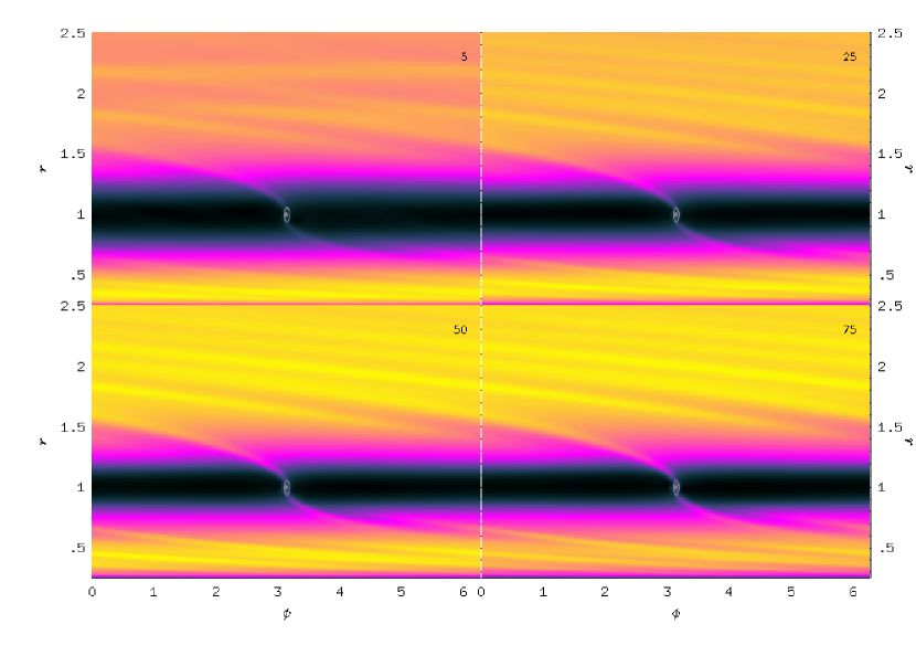
Figure 2: Grayscale plot of the surface density of the standard model at four different times, given in units of the orbital period of the planet. The scaling has been chosen such that black refers to $10^{-4}$ and white to $1.0$. The size of the planet’s Roche-lobe is indicated by the solid line around ($r=1,\varphi=\pi$)

The planet’s influence on the disc manifests itself in the creation of spiral disturbances in the surface density. The spiral pattern emerges very early during the evolution, already within the first 5 orbital periods, and the settles fast into a stationary state. The density is displayed in a gray scale plot in Fig. 2 at four different times. The final pattern consists of two tightly wound spirals on either side of the planet. On both sides, a primary spiral starts at the location of the planet. The secondary spirals start near the $L_{4}$ and $L_{5}$ points at $\varphi\approx\pi\pm\pi/3$ outside and inside of the planet. The tightness and the existence of additional spirals to the primary ones depend mainly on the equation of state, basically on the temperature in the disc (see below). Note, that in the corotating frame ($\Omega=\Omega_{p}$) the spirals are stationary and do not move through the grid. The density decrease (mass loss) inside of the planet is caused by the open inner boundary condition, where mass may leave the system to be accreted by the star.

The initial mass distribution approximates a disc already in a perturbed state including a gap.

Figure 3: The Surface density $\Sigma(r)$ of the standard model opposite of the planet at eight different times.

The gap also evolves slowly during the evolution and begins to narrow in the central parts somewhat from its initial radial extension. This is more clearly visible in Fig. 3, where $\Sigma(r)$ is plotted at a fixed angle $\varphi=0$ in opposition to the planet at different times. The initial axially symmetric profile is given by the solid line. Clearly visible are the different peaks produced by the spiral waves. The location and shape of the spirals are determined very early during the the evolution on dynamical timescales ($\Omega_{p}^{-1}$). The lowering of the density ($\Sigma$) in the outer parts is due to the accretion onto the protoplanet. While in the inner part ($r<1$) it is primarily due to mass loss through the open inner boundary.

Figure 4: Accreted mass onto the planet in dimensionless units, from the inside and outside of the planet for the standard model.

The mass accretion of the planet is plotted in Fig. 4, where it is distinguished whether the mass came from the outer parts ($r>1$) of the disc or the inner parts ($r<1$), respectively. In the computations we monitored continually the matter content in the disc regions exterior and interior of the planet’s orbital distance to the star. The mass accretion rate from the outer region approaches approximately a constant value after $t\approx 200$ (linear part of the dashed curve in Fig. 4), when the streams are fully developed. Initially the accretion rate is very small because of the pronounced imposed gap. The accretion from the inner region begins to diminish because of the loss of mass through the inner boundary. The actual physical value of the mass accretion rate depends on the assumed total mass initially in the disc, which is here in dimensionless units $M(0)=33.0$. Thus about $2.24\%$ of the total initial mass was accreted during 400 orbital periods of the planet.

From Fig. 5 we infer that indeed the mass accretion rate from the outside approaches a constant value, $\dot{M}_{P}=1.63\,10^{-3}$ in dimensionless units, where the unit of time is $P_{p}$ (Eq. 18). Assuming that the initial total mass in the disc (from $r_{\rm min}$ to $r_{\rm max}$) is $10^{-2}\rm M_{\odot}$ and that the planet orbits the star at a distance of $5.2$AU, then the unit of the mass flow rate as given in Fig. 5 (and subsequent figures) refers to $2.67\,10^{-2}M_{\rm Jup}/yr$. Hence, for our standard model we obtain after the initial transient the constant value

$$\dot{M}_{\rm P}(\mbox{out})=4.35\,10^{-5}M_{\rm Jup}/yr$$ (23)

for the equilibrium mass accretion rate from the outer disc onto a protoplanet with a mass ratio $q=10^{-3}$ and the disc parameter $\nu=10^{-5}$ and $H/r=0.05$.

Figure 5: Mass accretion rate onto the planet in dimensionless units, from the inside and outside of the planet for the standard model.

3.3 Influence of Numerical Parameters

The computation of the dynamics of the tenuous streams through the gap may depend on numerical effects such as artificial viscosity, resolution, boundary condition and so on. Thus, to obtain reliable estimates of the magnitude of a possible accretion rate through the gap, we kept the physical conditions of the model unchanged and varied only numerical input parameters. After these tests on the sensitivity of the results on the numerics we may concentrate later on the influence of the physical conditions on the gap dynamics.

Figure 6: Mass accretion rate from outside of the planet for different test cases with varying parameters (Table 2). The solid curve denotes the standard model (2q). The variations from the standard model are given by the labels.

Table 2: Parameter variations of from the standard model (Table 1) for the models displayed in figures 6, 7, 9, and 11

Name	Parameter	Description
2q	Standard	Reference Model
2q2	$v(r_{\rm min})=0$	Closed inner boundary
2q7	$\Omega=0$	Inertial frame
2q12	$r_{\rm min}=.4,r_{\rm max}=2.5$	Smaller physical domain
2s5	$256\times 256$	Higher resolution
Variations of Artificial Viscosity (Fig6., Fig. 7)
2q10	$C_{art}=2.0$	Four times larger bulk
		artificial viscosity
2n	$C_{art}=2.5$	Large Shear Art. Vis.
2l	$C_{art}=0.5$	Std. Shear Art. Vis.
2p	$C_{art}=0.1$	Low Shear Art. Vis.
2r	$C_{art}=0.0$	No Artificial Viscosity
Variations of Initial gap size (Fig. 9)
2q1		No initial gap
2q19		50% smaller gap
2q20		50% larger gap
Variations of accretion modeling (Fig. 11)
2q3	$f_{\rm red}=1/20$	Reduced accretion rate
2q6	$f_{\rm red}=5/2$	Enhanced accretion rate
2t5	$f_{\rm red}=1/2$	1/2 accretion radius
2t6	$f_{\rm red}=5/2$	1/2 accretion radius

In Fig. 6 the main results of our studies are displayed. The single variations from the standard models are named in the figure, and are listed in Table 2, all other parameter are identical to the reference model (2q) which is given by the solid line. Some of the irregularity in the results is caused by taking the derivative of data of the mass of the planet. Three models with a somewhat larger deviation (2r, dotted; 2s5 long dash-dotted; and 2q7 short-dashed) are explicitly labeled. The model with the vanishing artificial viscosity (2r) has a slightly higher accretion rate. The model with the larger resolution (2s5, only run to $t=200$) lies slightly below. Both of these models are noisier than the others due a too small artificial viscosity. The noise in $\dot{M}$ is usually larger for models with higher resolution because for smaller gridcells numerical effects (grid to grid oscillations) tend to increase. However, the artificial viscosity coefficient ($C_{art}$) has not been increased for model (2s5). The model that was run in the inertial frame (2q7) has possibly more numerical diffusion in the whole computational domain, as the planet and the spiral wave pattern are not stationary but move through the grid. Nevertheless, the agreement with the standard model is very good.

Figure 7: Mass accretion rate from outside of the planet for different types of artificial viscosity.

All other models lie very closely to the standard model. The model with the increased artificial viscosity (2q10, long-short dashed) and the model with the closed inner boundary (2q2, long dashed) give nearly identical results. The model with the smaller computational domain (2q12, short dashed-dotted) tests on one hand the influence of a variation the location of the radial boundaries (the reference model has $r_{\rm min}=0.25$ and $r_{\rm max}=4.0$) and on the other hand the influence of an increased resolution in the radial direction, since the same amount of radial grid points (128) was used. Both of these effects have basically no influence on the results. In summary, all models despite their parameter variations are consistent with the standard model.

We also would like to point out that the open inner boundary does not affect the accretion rate from the outside of disc. This indicates an independent mass flow from the inner and outer regions onto the planet with no or little interference where the inner mass accretion rate appears to be a given fraction of the outer one. In the computations we monitored continually the matter content in the disc regions exterior ($r>a$) and interior ($r<a$) of the planet’s orbital distance to the star. From the model with the closed inner boundary (2q2) we obtain that the mass accretion rate from the inner region $\dot{M}_{p}(in)$ also settles to a constant value with

$$\dot{M}_{p}(in)/\dot{M}_{p}(out)=3/5.$$ (24)

We concentrated here on the accretion from the outside since the mass on the inner side may be depleted during the evolution of the whole disc (for example by accretion onto the star or by an inner planet). These conditions were simulated by the open inner boundary. On the contrary, we may argue that the mass flow rate from the outer region alone gives a lower limit of the total accretion rate onto the system, for the given physical conditions.

Hence, we may conclude that we can detect a possible mass accretion rate onto a planet through a gap quite accurately, independent of numerical issues. And that a relatively moderate grid size of $128\times 128$ seems to be sufficient for an estimation of the mass accretion rate. However, the details of the flow in the vicinity of the planet need to be computed with much higher resolution. The time needed for reaching an equilibrium mass flow rate depends on the viscosity and is approximately $400$ orbits for $\nu=10^{-5}$.

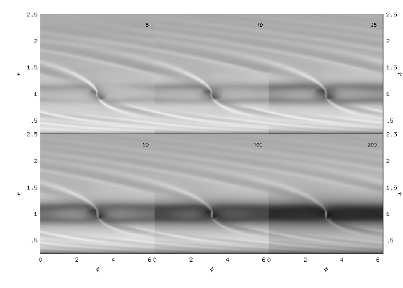
Figure 8: Grayscale of the surface density of the model with no initial gap at six different times.

3.3.1 Remarks on the artificial viscosity

Since numerical instabilities tend to originate in the low density gap region, there is, as has been seen already in the preceding paragraph, the necessity of using an artificial viscosity. As mentioned above we found it necessary that this additional viscosity is only applied to the bulk viscosity part, and not the shear viscosity components. To illustrate the reasoning, we ran some models with a shear artificial viscosity having different magnitudes of the coefficient $C_{\rm art}$. To distinguish this effect, it is not very useful to look at the two-dimensional flow fields since they are always very similar. But the crucial mass accretion rate tends to have a strong sensitivity to this purely numerical issue.

From Fig. 7, where the mass accretion rate for different models with a varying type of artificial viscosity is plotted, it is apparent that in the models using an artificial viscosity which operates also on the shear contributions of the viscous stress tensor, the mass accretion rate depends strongly on the magnitude of the viscosity coefficient $C_{\rm art}$. The model having the same $C_{\rm art}$ as the reference model (2l, short dashed line) has about a three times larger $\dot{M}_{p}$ rate. Additionly, the mass accretion rate depends strongly on the magnitude of the coefficient. An increase/decrease in $C_{\rm art}$ leads subsequently to an increase/decrease in the accretion rate $\dot{M}_{p}$. The model (2n, dotted) has a five times higher $C_{art}$, resulting in such a large fictitious mass accretion onto the planet that the mass reservoir outside of the planet begins to deplete. Only for very low values of $C_{\rm art}$ (2p, long dashed) the curves seems to approach the zero artificial viscosity value (2r, short dashed dotted). Apparently the shear artificial viscosity acts as an additional physical viscosity influencing strongly the estimated mass accretion rate.

In case of an artificial viscosity only operating on the bulk parts of the viscous stress tensor (2q10, long dashed dotted) there is no apparent dependence of the accretion rate on $C_{\rm art}$; the curve with $C_{\rm art}=2.0$ which is four times standard, is nearly identical to the zero artificial viscosity case. One may argue here, that if runs with no artificial viscosity are possible why bother at all. The reason is that for higher resolution, or for different physical viscosities the usage of an artificial viscosity may be warranted to prevent numerical instabilities. Thus, we conclude that the bulk artificial viscosity is the selection of choice, since firstly, it does not change important physical effects, and secondly it is sufficient to keep the numerical scheme stable. From these tests we may also infer that the mass accretion depends crucially on the type of viscosity used, and will be reduced/increased for smaller/larger physical viscosity coefficients (see below).

3.3.2 Varying the initial condition

The results displayed so far indicate an asymptotic, constant value for the mass accretion rate (Eq. 23) given a specified value of the initial mass in the region outside the planet. As these results were obtained with an initial gap around the planet, it is interesting to study the situation with no such initially imposed gap. Hence, we constructed models with varying extensions of the initial gap. One model (2q1) had initially no gap at all but rather the equilibrium surface density distribution $\Sigma(r)\propto r^{-1/2}$ throughout the whole computational domain. Two additional models with a $50\%$ smaller and larger radial initial extension of the gap have been calculated (see Table 2).

In the case with no initial gap at all the torques generated by the planet begin to open the gap from ’scratch’ and at $t=5$ the spiral wave pattern and the general shape of the gap are already clearly visible (Fig. 8). In the following evolution the gap clearing proceeds rapidly where the regions near the Lagrangian points $L_{4}$ and $L_{5}$ which are located at $\Delta\varphi=\pm\pi/3$ from the planet have the longest clearing time. The final shape of the gap and spiral pattern (eg. at $t=200$) is nearly indistinguishable from the reference model with an initial gap. The mass accretion rate is of course initially very high for this model but for later times is approaching the accretion rate of the previous standard model (Fig. 9). The $\dot{M}_{p}$ curves of the models with the 50% smaller/larger initial gap size also approach the standard curve from above/below (Fig. 9). Hence, the models seem to converge to the same final equilibrium accretion mass accretion rate $\dot{M}_{p}$ despite of the very different initial conditions.

The process of the gap clearing for the model with no initially imposed gap is exemplified in Fig. 10, which should be compared to the standard model in Fig. 3 above. Initially the gap begins to clear fastest at radii slightly larger and smaller than the planet, i.e. at its boundaries where the tidal torques are highest. Only at very late times the density in the central region of the gap reaches the plateau present in the standard model from the very beginning. Clearly visible is again the stationarity of the location of the spirals which appear at specific radii after very few orbits and remain stationary there throughout the evolution.

From the test models, with varying initial gap sizes it is clear that evolution takes place on a viscous time scale, which is several thousand orbits for the constant viscosity $\nu=10^{-5}$.

Figure 9: Mass accretion rate from outside of the planet for the standard model and models with different gap sizes.

Figure 10: The Surface density $\Sigma(r)$ opposite of the planet (at $\varphi=0$) for the model with no initial gap (2q1). The solid line indicates the initial density distribution.

3.3.3 Influence of the accretion radius inside the Roche lobe

Figure 11: Mass accretion rate for different accretion radii within the Roche lobe.

In section 3.1 we explained how the accretion process onto the planet is modeled numerically. The value of the reduction factor $f_{\rm red}$ may play an important role in determining the accretion rate onto the planet. To check its influence we ran models where $f_{\rm red}$ has been varied (see Table 2). The results (Fig. 11) indicate that firstly a larger increase (5 times bigger in model 2q6) does not alter the achieved maximum accretion rate significantly, while a ten times smaller factor (2q3) reduces the final accretion rate only by about $40\%$. In all the calculations presented so far the accretion radius (i.e. the domain in which mass was taken out to simulate accretion) was the whole size of the Roche lobe, with an enhanced accretion within the inner half of the Roche lobe. Two additional models where the size of the accretion region was reduced to only the inner half of the lobe with an enhancement in the inner quarter were run in the inertial frame. In the first model (2t5) the reduction factor was kept (despite the smaller accretion radius) at $f_{\rm red}=0.5$ while in the second model (2t6) it was increased by a factor of 5. While the first model (2t5) has about a $30\%$ smaller accretion rate, the latter model reaches the same value as the standard model.

We may conclude that independent of the details of the modeling of the accretion process within the planet’s Roche lobe, there exists a well defined maximum accretion rate as given by our standard model (Eq. 23). If the planet does not fill its Roche lobe entirely this maximum rate may be reached. For comparison, Jupiter’s radius is only $1.34\,10^{-3}$ of its Roche radius. This maximum achievable accretion rate may be compared to the equilibrium rate of a stationary accretion disc which is given by

$$\dot{M}_{\rm acc}=3\pi\nu\Sigma.$$ (25)

In dimensionless units we obtain $\dot{M}_{\rm acc}=5.9\,10^{-4}$ (for $\Sigma=1.$ and $\nu=10^{-5}$) which is about 2.8 times smaller than our maximum accretion rate. At a first glance this may be surprising, but one has to remember that (25) refers to an undisturbed disc. Boundary effects in an accretion disc (for example near the central star) may increase the equilibrium accretion rate considerably (eg. Frank, King & Raine 1992). The presence of a planet in the disc perturbes the disc flow and acts as a inner boundary to the outer parts of the disc at $r>a$, modifying the relation (25). Note, with boundary effect we do not refer to the conditions at the inner boundary ($r_{\rm min}$) of the computational domain (closed or open) which do not have any influence on the accretion rate from the outside as shown above. Additionally, an increased radial pressure gradient in the gap region will increase the accretion rate (see Sect. 3.5 below). Both, the effect of the planet on the outer disc, and pressure effects may account for a possible slight enhancement of $\dot{M}_{p}$ above $\dot{M}_{\rm acc}$.

Having tested the effects of several numerical aspects of the code and boundary and initial conditions we come now the influence of the physical properties of the disc.

Table 3: Variations of the physical viscosity and vertical thickness for the models displayed in Figures 12 and 13, and Table 4. For the reference model see Table 1

Name	Parameter	Description
Variations of the viscosity (Fig. 12)
2q	$\nu=1\,10^{-5}$	Reference Model ($H/r=0.05$)
2q4	$\nu=4\,10^{-5}$	Four times larger visc.
2q14	$\nu=2\,10^{-5}$	Two times larger visc.
2q15	$\nu=5\,10^{-6}$	Two times lower visc.
2q5	$\nu=2.5\,10^{-6}$	Four times lower visc.
2q23	$\nu=1\,10^{-6}$	Ten times lower visc.
2y1	$\nu=0$	Zero viscosity
2x1	$\alpha=0.004$	$\alpha$-type viscosity
2x	$\alpha=0.001$	$\alpha$-type viscosity
Variations of the disc height (Fig. 13)
2qz	$H/r=0.1$	Two times larger $H/r$
2q8	$H/r=0.075$	1.5 times larger $H/r$
2q17	$H/r=0.025$	2 times lower $H/r$

3.4 Influence of the physical viscosity

The calculations presented so far have been performed with the constant kinematic viscosity $\nu=10^{-5}$. It is to be expected that the mass accretion rate depends on the magnitude of the physical viscosity. Thus, we performed different calculations where the kinematic viscosity coefficient $\nu$ was varied from its standard value $10^{-5}$. For comparative purposes we also used an $\alpha$-type viscosity with two different values of $\alpha$. For all the models the remaining physical parameters, in particular the scale height (temperature), are identical to the standard model (2q). Note also, that the initial density profile and the gap size was identical for all models. The model parameter are given in Table 3, The main results are displayed in Fig. 12. Note, that the two models with the lowest (2q23) or even zero (2y1) viscosity were evolved for about 1000 orbits. They are not included in the figure since their accretion rates which are stated in Table 4 are very small.

Figure 12: Mass accretion rate from the outside of the planet for different physical viscosities.

Obviously the mass accretion rate depends strongly on the magnitude of the viscosity. The decrease in $\dot{M}_{p}$ for the larger viscosity models (2q4, 2q14) is a result of the mass depletion of the outer region of the disc.

From the results we construct Table 4, where the accretion rates are listed for different values of the viscosity (both in dimensionless units, where $[\dot{M}_{p}]=2.67\,10^{-2}M_{\rm Jup}$/yr). Also stated is the growth timescale $\tau_{g}$ of the planet. The values of the accretion rate for the higher viscosity models (2q4, 2q14) are taken at the maximum value before mass depletion sets in.

Table 4: Dependence of the mass accretion rate on the viscosity, both given in dimensionless units. In the third column the growth time scale $\tau_{g}=m_{\rm p}/\dot{M}_{\rm p}$ is given in years for a one Jupiter mass planet at a distance $r_{\rm J}$ from the star.

Model	Viscosity	$\dot{M}_{p}(out)$	$\tau_{g}$
	[$10^{-5}$]	[$10^{-3}$]	[yrs]
2y1	0	0.0003	$1.2\,10^{8}$
2q23	0.10	0.03	$1.2\,10^{6}$
2q5	0.25	0.18	$2.1\,10^{5}$
2q15	0.50	0.64	$5.8\,10^{4}$
2q	1.00	1.63	$2.3\,10^{4}$
2q14	2.00	3.4	$1.1\,10^{4}$
2q4	4.00	7.0	$5.4\,10^{3}$
2x	$\alpha=0.001$	.28	$1.3\,10^{5}$
2x1	$\alpha=0.004$	2.2	$1.7\,10^{4}$

We infer that the mass accretion rate for larger viscosity depends approximately linearly on the viscosity with an offset (zero $\dot{M}_{p}$ at $\nu\approx 1.6\,10^{-6}$). For lower viscosities ($\nu\raisebox{-2.58334pt}{$\stackrel{{\scriptstyle{\displaystyle<}}}{{\sim}}$}5\,10^{-6}$) however, the $\dot{M}_{p}$ rates are dropping much faster than linear. For a ten times lower viscosity (2q23, $\nu=10^{-6}$) the accretion rate onto the planet is reduced by a factor of about 50. The model with no physical viscosity (2y1) has an accretion rate which is again 100 times smaller. This is an additional indication of the low numerical viscosity in the numerical scheme.

For the models having a constant $\alpha$-type viscosity (cf. Eq. 15), we find that the model with $\alpha=0.004$ (2x1) refers approximately to the standard model with $\nu=10^{-5}$. Which was expected from the initial setup, where we chose for $\alpha$ such a value that the two viscosities agree at the radius $r=1$. The ratio of $\dot{M}_{p}$ between $\alpha=0.004$ and $\alpha=0.001$ is similar to the one between $\nu=1.0\,10^{-5}$ and $\nu=0.25\,10^{-5}$. We note, that the accretion rate for the $\alpha=0.001$ model (2x) refers to $7.5\,10^{-6}M_{\rm Jup}/yr$.

In the last column the growth time scale $\tau_{g}=m_{\rm p}/\dot{M}_{\rm p}$ is given in years which may be compared to the calculations of Bryden et al. (1998). The accretion time scale has to compared to the viscous evolution time of the disc which is given for the constant viscosity by

$$\tau_{\nu}=1.9\nu^{-1}\mbox{yrs}.$$ (26)

Hence we find that for $\nu=10^{-6}$ the two time scales are comparable, while for larger $\nu$ the accretion timescale is smaller than the viscous evolution time scale (for $H/r=0.05$, and $q=10^{-3}$).

3.5 Influence of the scale height of the disc

Here we study the consequences of a varying thickness (temperature) of the disc on the mass accretion rate keeping the viscosity coefficient fixed at $\nu=10^{-5}$. The model parameter are summarized in Table 3.

Figure 13: Mass accretion rate from the outside of the planet for different values of the disc thickness.

From Fig. 13 we infer that (at least for the models having a smaller $H/r$) the mass accretion rate depends linearly on the chosen value of $H/r$ with an offset at $\dot{M}_{\rm p}\approx 8\,10^{-4}$. The variations in the thickness were chosen with fixed linear spacing which led approximately to a linear change in the accretion rate. The model with the largest $H/r=0.1$ (2z) shows a value slightly too small compared with this relationship. This deviation from the linear behaviour may be caused firstly by the mass depletion of the outer parts and secondly by non-linear effects which begin to set in for larger internal pressure of the disc. For the given grid resolution it is not possible to study models with a smaller $H/r$ value, since then the radial pressure scale length would be smaller than the size of one gridcell.

3.6 Influence of the equation of state

So far an isothermal equation of state has been used, where the temperature profile in the disc had a given $\propto r^{-1}$ dependence. To simulate possible cooling effects and their influence on the viscosity we performed some additional calculations using a polytropic equation of state (7). An adiabatic exponent $\gamma=2$ was used and the constant $K$ has been set to such a value that the disc thickness is approximately $0.05$ at the radius $1$. In dimensionless units this refers to $K=0.0025$. The viscosity prescription was also varied in these models. Starting from the standard constant value $\nu=10^{-5}$, models with no physical viscosity at all (4y) and with an $\alpha$-type viscosity were considered.

Figure 14: Mass accretion rate from the outside of the planet for polytropic models using different parameter.

As can be seen from Fig. 14, the model using a constant $\nu$ but a polytropic equation of state (4l) follows the reference model closely. The constant $K$ was chosen slightly too small for a better agreement. Choosing an $\alpha$-type viscosity the mass accretion rate is also for the larger value $\alpha=0.004$ (model 4x1) reduced from the constant $\nu$ case (cp. Fig. 12). A value of $\alpha=0.001$ (4x) lies also below the isothermal model. The data for the $\alpha=0.004$ model are relatively noisy, most likely because non-linear effects caused by the strong dependence of pressure and viscosity on the surface density begin to set in. A detailed analysis of these phenomenon lies outside of the scope of this paper.

The general trend of an $\alpha$-type viscosity prescription together with a polytropic equation of state is obvious, however. For polytropic models the pressure is linked directly to the density, and because the density and pressure scale height are very small in the gap, this leads to a reduction of the viscosity for an $\alpha$-type law, and consequently to a lowering of the mass accretion rate onto the planet. This does not occur in case of the isothermal equation of state (see model 2x, 2x1 in Fig. 12), where the temperature in the gap is not reduced. Additionally, for an isothermal equation of state the density in the gap can never vanish, but it can for a polytropic equation of state. For comparison we calculated also a model with vanishing physical viscosity (4y). As expected, the mass accretion rate in this case effectively vanished. Again, a comparison isothermal model with zero physical viscosity was run for about 1000 orbits which shows very low accretion onto the planet $\dot{M}_{p}<3\,10^{-7}$ (see Table 4).

3.7 The size of the gap

Figure 15: Radial surface density distribution at $\varphi=0$ in opposition to the planet for various viscosities stated in units of $1.0\,10^{-5}$ at $t=400$.

Figure 16: Radial surface density distribution at $\varphi=0$ in opposition to the planet for various disc temperatures for $t=400$.

Aside from the mass accretion rate onto the planet, the physical extent of the gap is important as it determines observational properties of protostellar discs. The radial size of the gap is determined by the mass of the planet and the properties (viscosity, scale height) of the disc. Keeping the temperature in the disc fixed ($H/r=0.05$) and varying the viscosity by a factor of 4 from the standard value we find that the gap size varies only very slightly with viscosity (Fig. 15). The data in Fig. 15 are taken at the angle $\varphi=0$ opposite of the planet. The inner gap size at the radial location $r=1$ of the planet is decreasing with increasing viscosity, while the outer part at about $r=1.55$ is increasing with larger $\nu$. The location of the maxima, i.e the location of the spirals is not visibly affected by the magnitude of the viscosity. The range of $\nu$ covers $2.5\,10^{-6}$ to $4\,10^{-5}$, i.e. a factor of $16$. The first, innermost bump at $r=1.4$ is created by the secondary spiral (cf. Fig. 2), and then primary and secondary spirals interchange. A higher viscosity causes a stronger mass accretion from the outside, and hence a lowering of the density in the outer parts. The inner region ($r<1$) is strongly influenced by mass loss through the inner boundary. A variation of the non-physical model parameter (artificial viscosity resolution etc.) as presented in Fig. 6 does not alter the size and shape of the gap and spirals at all.

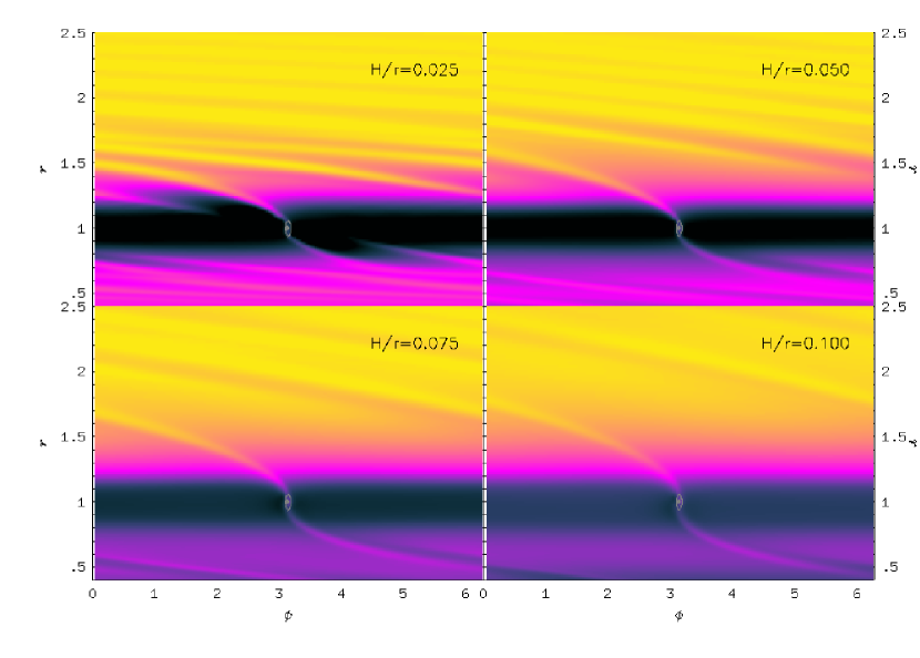
Figure 17: Surface density distribution for four different values of $H/r$ at $t=400$. The density is scaled as $\Sigma^{1/4}$ between $4.2\,10^{-3}$ and $0.90$.

On the contrary, a variation of the vertical disc thickness has a much bigger effect on the structure of gap and spirals (Fig. 16). The smaller the temperature the narrower is the gap and the spirals are more tightly bound. The density enhancement in the spirals above the surrounding is also more pronounced for lower $H/r$, as can be seen most clearly from the coolest disc (dashed-dotted line). At higher temperatures the secondary spiral disappears. In the plot it is hardly visible anymore for $H/r=0.075$ (short dashed) and not at all for $H/r=0.1$ (dotted). The variation of the tightness of the spirals as a function of $H/r$ is clearly visible in Fig. 17, where gray scale contour plots of the surface density are displayed for the four different values of $H/R$ (but fixed $\nu=10^{-5}$) at the same time of $400$ orbits. A smaller $H/r$ value clearly leads to a more pronounced gap with a lower density within the gap region.

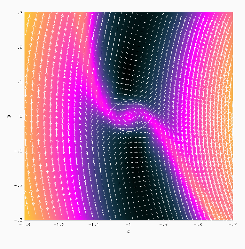
Figure 18: Flow field in the vicinity of the planet in a reference frame corotating with the planet. The length of the velocity vectors scale logarithmically.

3.8 The flow in the vicinity of the planet

The structure of the flow near the protoplanet can only be studied by using higher resolution models. Here we used a model (2q16) with $R_{\rm min}=0.4$, $R_{\rm max}=2.5$ and a resolution of $128\times 442$ gridcells where the radial spacing is logarithmic such that each gridcell has an approximately square shape in $x-y$ in the corresponding coordinates. Caused by the higher resolution it was not possible to follow the whole evolution over several hundred orbits, instead we ran the model upto $t=100$. As seen above, the flow field at this time has become approximately stationary and represents quite accurately the flow at later times.

We would like to point out that from the flow field it is apparent that the mass accretion does not occur along the spiral arms (which may be guessed by purely looking at the density graphs in the previous plots). These spiral arms are in fact trailing shock waves. The mass supplied to the Roche lobe of the planet comes from material following the stream lines of the horseshoe orbits in the vicinity of the planet. From Fig. 18 we notice that some material follows orbits that enter the Roche lobe from regions with are lying outside ($r>a$) and inside ($r<a$) of the planet. This matter is then allowed to be accreted by the planet. As mentioned above, the accretion rate from inside is about 3/5 of the one from the outside when the inner boundary is closed to mass flow. The inner rate is reduced significantly however by the open inner boundary, which is why we displayed primarily only the value from the outside.

The flow field (Fig. 18) near the planet (the central white dot), whose Roche lobe is indicated by the solid line, shows that the mass and consequently angular momentum is accreted in such a way to induce a prograde rotation of the protoplanet, as it is observed in the solar system for all massive planets with the exception of Uranus. The numerical resolution within the Roche lobe is still not very high, but one can notice nevertheless that the matter orbits the planet. Whether this circulation around the planet (the proto-Jovian disc) is Keplerian cannot be determined from the model, since the smoothing length modifies the potential within the Roche lobe. Mass does not really accumulate within the Roche lobe as it is taken out continually to simulate accretion onto the central planet.

Finally, we mention that a comparison model (with standard resolution) where no mass accretion onto the planet was taken into account ($f_{\rm red}=0$) produces a hydrostatic density distribution within the Roche lobe on dynamical time scales which prevents further mass accumulation. The flow field, which is similar to Fig. 18, allows in principle for mass to be transferred across the gap. We find in this case a net mass flow from radii outside of the planet across the gap to radii smaller than $a$ of about 1/7 of the standard value (23) which is substantially smaller than the equilibrium accretion rate (25).

4 Conclusions

We have studied the structure of an accretion disc in a protostellar environment under the perturbing influence of an embedded protoplanet. In particular we were interested in the possibility of continued accretion of mass after the opening of a gap by the planet. Starting from a standard model with a constant kinematic viscosity coefficient of $\nu=10^{-5}$ and a vertical thickness of $H/r=0.05$, we first carefully analyzed the the possible influence of numerical properties such as resolution, artificial viscosity and rotating coordinates.

Grid resolution and the change from a corotating coordinate system to an inertial frame do not alter the physical conclusions, i.e. have no or very little influence on the mass accretion rate, and the structure of the gap and trailing shocks. However, the artificial viscosity has to be treated carefully, and it turned out that it has to act only on the bulk part of the viscous stress tensor. This has implications for calculating similar situations where small deviations from the mean value of the shear in the underling basic flow are of importance.

The main result of the following calculations has clearly shown that for all viscosities there is still some accretion onto the planet taking place, even though the rate is greatly reduced for a very low viscosity. The limiting mass of a planet is then determined by the competing accretion and viscous time scales (see below), and of course by the available mass reservoir in the surrounding protostellar disc. In case of an existing gap the accreted mass originates from material following streamlines of the horseshoe orbits at the inner and outer edge of the gap (Fig. 18), where the outside accretion rate is approximately 1.5 times as large as from the inside (Eq. 24).

There appears to exist a well defined given maximum accretion rate (obtained by allowing maximum accretion within the planet’s Roche lobe) depending only on viscosity and temperature in the disc. For a disc viscosity $\alpha=10^{-3}$ and vertical thickness $H/r=0.05$ we estimate the timescale for the accumulation of one Jupiter mass to be of order hundred thousand years. For a larger(smaller) viscosity and disc thickness this accretion rate is increasing(decreasing). The main ingredient required for such a gap accretion is a non vanishing viscosity within the gap region. The results with a polytropic equation of state show that in the case of a viscosity linked to the density (which is very low in the gap) the accretion rate is smaller. However, one may argue that in a realistic situation the viscosity, if for example driven by some sort of MHD turbulence, is also sufficiently large in optically thin regions which would allow further accretion.

For smaller viscosities $\nu\raisebox{-2.58334pt}{$\stackrel{{\scriptstyle{\displaystyle<}}}{{\sim}}$}10^{-6}$ the mass accretion rate through the gap onto the planet is markedly reduced (Table 4), and the corresponding accretion time scale becomes larger than the viscous evolution time of the disc. Additional, separate calculations (Bryden et al. 1998) have shown, that the mass accretion rate onto the planet decreases with larger $q$, and become for $q=10^{-2}$ very much longer than $\tau_{\nu}$. Hence, the presented calculations show that, for the typical evolution time scales of protostellar discs ($\tau_{\nu}\approx 10^{6}$yrs), the final mass of the planet appears to be in the range $1-10M_{\rm J}$ consistent with the observations.

The outlined accretion process onto protoplanets can only occur in a region of the protoplanetary disc with a sufficiently large enough mass reservoir, typical for the protostellar disc at a distance of a few AU from protostar. As some of the extrasolar planets (51 Peg type planets) have distances to their stars which are very much smaller than 1 AU, these planets must then have migrated to their presently observed position (Lin, Bodenheimer & Richardson 1996; Ward 1997).

Finally, we would like to point out that our conclusions concerning the time scale of the accretion process are slightly uncertain, as they depend on the mass density in the disc surrounding the planet which scales out of the problem. The numbers stated always refer to a disc having 0.01 $\rm M_{\odot}$ in the range 1.3 to 20.8 AU. Additionally, the quoted rates are a lower limit as we only considered here the accumulated mass from the outer parts of the disc. Another problem relates to the accretion process within the planet’s Roche lobe. Only if viscous effects in the proto-Jovian disc are sufficiently high to create an $\dot{M}$ as large as the supplied rate from the protostellar disc, the maximum accretion rate (Eq. 23) can be achieved. The evolution of the proto-Jovian disc is an outstanding problem which needs to be addressed. The masses of the extrasolar planets are also lower limits as they still include the uncertain inclination of the orbit to the line of sight of the observations. Statistically one may expect them to be a factor 1.3 higher.

Further problems, such as the details of the flow in the vicinity of the planet, the angular momentum transfer, the influence of a non-vanishing eccentricity or orbital inclination of the planet, the modeling of energy transfer in the disc, and other issues are beyond the scope of present study. Some of these future investigations will even require fully three dimensional calculations.

References

- [1] Artymowicz, P., Lubow, S.H., 1994, ApJ, 421, 651.
- [2] Artymowicz, P., Lubow, S.H., 1996, ApJ, 476, L77.
- [3] Boss, A. P., 1996, Physics Today, 49/9, p32.
- [4] Bryden G., Chen, X., Lin, D.N.C, Nelson, R.P. & Papaloizou, J.C.B., 1998, submitted to ApJ, preprint.
- [5] Butler, R.P. & Marcy, G.W., 1996, ApJ, 464, L153.
- [6] Cochran, W., 1997, Physics World, July 1997, p31.
- [7] Flebbe, O., Münzel, S., Herold, H. Riffert, H., and Ruder, H., 1994, ApJ, 431, 754.
- [8] Frank, J., King, A. & Raine, D., 1992, Accretion Power in Astrophysics, 2nd Edition, Cambridge Univ. Press.
- [9] Glanz, J., 1997, Science, 276, 1336.
- [10] Goldreich P. & Tremaine S., 1980, ApJ, 241, 425.
- [11] Hoyle, F., 1946, MN, 106, 406.
- [12] Kley W., 1989, A&A, 208, 98.
- [13] Kley W., 1998, A&A, 338, L37.
- [14] Korycansky, D. G., Papaloizou J.C.B., 1996, ApJS, 105, 181.
- [15] Lin, D.N.C., Papaloizou, J.C.B., 1980, MNRAS, 191, 37.
- [16] Lin, D.N.C., Papaloizou, J.C.B., 1986, ApJ, 307, 395.
- [17] Lin, D.N.C., Papaloizou, J.C.B., 1993, in Protostars and Planets III, Ed. E.H. Levy, J.I.Lunine, U. Arizona P., Tucson.
- [18] Lin, D.N.C., Bodenheimer, P. & Richardson, D.C., 1996, Nature, 380, 606.
- [19] Marcy, G.W. & Butler, R.P., 1996, ApJ, 464, L147.
- [20] Marcy, G.W. & Butler, R.P., 1998, to appear in Cool Stars, Stellar Systems, and the Sun Eds. R. Donahue & J. Bookbinder.
- [21] Mayor, M. & Queloz, D., 1995, Nature, 378, 355.
- [22] Mazeh, T., Mayor, M., & Latham, D.W., 1997, ApJ, 478, 367.
- [23] Miki, S., 1982, Prog. Theor. Phys., 67, 1053.
- [24] Papaloizou, J.C.B. & Lin, D.N.C., 1984, ApJ, 285, 818.
- [25] Pringle, J.E., 1981, ARA&A, 19, 137.
- [26] Sekiya, M., Miyama, S.M. & Hayashi, C., 1988, Prog. Theor. Phys., 96, 274.
- [27] Shakura N.I., Sunyaev R.A., 1973, A&A, 24, 337.
- [28] Ward, W., 1997, Icarus, 126, 261.