The Reaction Rate Sensitivity of Nucleosynthesis in Type II Supernovae
Abstract
We explore the sensitivity of the nucleosynthesis of intermediate mass elements ( A ) in supernovae derived from massive stars to the nuclear reaction rates employed in the model. Two standard sources of reaction rate data (Woosley et al. 1978; and Thielemann et al. 1987) are employed in pairs of calculations that are otherwise identical. Both include as a common backbone the experimental reactions rates of Caughlan & Fowler (1988). Two stellar models are calculated for each of two masses: 15 and 25 M⊙. Each star is evolved from core hydrogen burning to a presupernova state carrying an appropriately large reaction network, then exploded using a piston near the edge of the iron core as described by Woosley & Weaver (1995). The final stellar yields from the models calculated with the two rate sets are compared and found to differ in most cases by less than a factor of two over the entire range of nuclei studied. Reasons for the major discrepancies are discussed in detail along with the physics underlying the two reaction rate sets employed. The nucleosynthesis results are relatively robust and less sensitive than might be expected to uncertainties in nuclear reaction rates, though they are sensitive to the stellar model employed.
and
1 INTRODUCTION
Two major efforts to model nucleosynthesis in massive stars have operated in parallel for a number of years (e.g., Woosley & Weaver 1995; Thielemann, Nomoto, & Hashimoto 1996). These groups have differed in the stellar physics they employed - convection theory, treatment of stellar energy generation, starting point (the main sequence for the former, helium cores for the latter), and how the supernova explosion was simulated. They also differed, especially for elements heavier than silicon, in their choice of nuclear reaction rates. Nomoto and his collaborators have always used the Hauser-Feshbach calculations of Thielemann et al. (1987; henceforth TAT). So far, Woosley & Weaver have used those of Woosley et al. (1978; henceforth WFHZ).
Considering the many differences between the models, it is comforting (perhaps even surprising) that the predicted nucleosynthetic yields from these two groups agree as well as they do, but detailed comparison does reveal discrepancies. Here we shall segregate those differences that exist because of the dichotomy of stellar models from those reflecting purely the choice of nuclear physics. We shall also discuss the underlying assumptions in each reaction rate set and why the two differ.
We begin by describing (2) the two approaches to stellar evolution and, briefly, the two rate sets (pending a more thorough review in 4). Section 3 presents new yields for some hybrid models - stars evolved using the KEPLER code of Weaver, Zimmerman, & Woosley (1978) and exploded as described in Woosley & Weaver (1995), but using rates from both groups (TAT & WFHZ). In addition to helping to understand why calculations of the two groups differ, the use of two independent sets of reaction rates in identical stellar models helps determine the (nuclear physics portion of the) error bar one should assign to nucleosynthesis studies of this sort. We find, in general that it is relatively small.
In 4, we examine in greater detail the nuclear physics that produced the two reaction rate sets, specifically the input data and physical assumptions employed in two globally parameterized Hauser-Feshbach calculations by Woosley et al. (1978) and Thielemann et al. (1987). Previously unpublished comparisons to experimental rates are given along with mutual comparisons of the two sets.
Section 5 then discusses the differences in stellar yields in light of the results of 4 as well as the known differences in the stellar models. In 6, we summarize and conclude.
2 Previous Models and the Rates They Employ
2.1 A Tale of Two Stellar Models
The nucleosynthesis calculations provided to the community by Thielemann, Nomoto & Hashimoto (1996, hereafter TNH) are based on the stellar evolution calculations of Nomoto & Hashimoto (1988) for massive stars. These calculations were extended to a larger grid of progenitor masses by Hashimoto et al. (1993). Both works followed the evolution of helium cores of fixed mass (omitting hydrogen burning and complications of mass loss and red giant formation) and both used the Schwarzschild criterion for convective instability. The nuclear energy generation and nucleosynthesis within a structural iterative loop (stellar evolution time-step) was evaluated using a reduced reaction network adopted to the appropriate burning stages (for details see Thielemann, Hashimoto, & Nomoto, 1990; Nomoto & Hashimoto 1988; Hashimoto, Hanawa, & Sugimoto 1983; and Hashimoto, 1995). A 30 isotope network was used from He to oxygen burning that included essentially only stable nuclei up to Ca and did not include neutron-rich nuclei. Silicon burning, a much more complicated stage of stellar burning in which equilibrated strong flows must be followed and weak interactions on trace isotopes are important, was treated in a different way. During the onset of silicon burning a 148 isotope network was employed, extending to Ca and including also unstable and neutron-rich species. After partial burning of Si, when quasi-equilibrium in the Si-group was attained, the calculation switched to using tables of the relevant quantities evaluated previously with a 299 isotope network given in Thielemann, Hashimoto, & Nomoto (1990). The tables gave for each instant of silicon burning at density, , temperature, , and electron mole number,, the appropriate energy generation rate, silicon depletion rate, and time derivative of . Technically this was done by interpolating quantities from prior calculations for a grid of densities, temperatures, , and Si mass fraction. The individual abundances of the isotopes could be obtained, if necessary, from quasi-equilibrium at the same , , , and .
Such a treatment led to an approximately correct energy generation rate during all stages of stellar evolution and also kept track of the major abundances. Limitations in this network, however, which e.g. did not contain all production or depletion reactions of 26Al, meant that it could not give reliable answers for the abundances of such isotopes. Similar limitations on the neutron-rich side of the (stellar evolution) network did not permit the -process to be calculated. “Post-processing calculations” by Prantzos, Hashimoto & Nomoto (1990) gave an indication of what -processing might be expected during He-burning, but this study centered on the major -process nuclei beyond Fe (and not lighter elements like Si, P, S, Cl, Ar, K, Ca, and Ti as discussed in Käppeler et al. 1994)
This treatment differed in many ways from Woosley & Weaver (1995, hereafter WW95). These authors also made use of a smaller 19 isotope network to calculate energy generation during hydrogen, helium, carbon, neon, and part of oxygen burning. Though the matrix contained only 19 species, assumed steady state links for about a dozen other nuclei made it the equivalent of a larger network of about 30 isotopes (Weaver, Zimmerman, & Woosley 1978). After the oxygen abundance declined, during central oxygen burning, to below 4%, the transition was made to a larger quasi-equilibrium network of 137 isotopes. This network was converged during each iterative cycle of the stellar code and accounted for most of the computational expense of the entire evolutionary calculation. In addition, Weaver et al. (and subsequently WW95) used a different criterion for convective instability, the Ledoux criterion plus semi-convection in the regions that were Schwarzschild unstable but not Ledoux unstable. This contributed significantly to the variable iron core masses obtained by the two groups for a given helium core mass (in the Ledoux criterion a barrier inhibits convection, in the Schwarzschild criterion it does not). Finally, WW95 treated their large network nucleosynthesis in a different way. A reaction network of 200 isotopes (large by the standards of the time) was carried in a “co-processing” mode in each zone throughout the entire stellar evolution. Thus the converged T and of each stellar model was used to update this network at each time step, and most importantly, convective mixing was carried out in the co-processed abundance set wherever appropriate. The -process up to A=65 was also calculated. This sort of detail was missing in the presupernova models of Nomoto & Hashimoto (1988) and Hashimoto et al. (1993), and thus restricted the information available from the presupernova evolution when it came time to calculate the explosion.
During the explosive part of the modeling, there were differences as well, though not so dramatic. The size of the nuclear networks for this phase have been discussed in WW95 and in Thielemann, Hashimoto & Nomoto (1990). Because of persistent uncertainties in modeling the explosion of Type II supernovae as well as the practical need to explore a wide range of stellar models, both groups simulated explosions artificially. WW95 made use of an inward (during in-fall, before the explosion) and outward (after the induced explosion) moving piston with a velocity which caused a final kinetic energy of the ejecta of erg. The details of this method were first described in Woosley & Weaver (1986) and are discussed in detail in WW95. Thielemann, Hashimoto & Nomoto (1990), Hashimoto et al. (1993), TNH, and Nomoto et al. (1997) made use of a ”thermal bomb”, i.e. introducing thermal energy in the form of a temperature enhancement inside the Fe-core of the progenitor star. The thermal energy was also chosen in such a way to attain a total kinetic energy of the ejecta of erg. While WW95 obtained a mass cut between ejecta and neutron star (which determined the total amount of 56Ni ejected) from their choice of piston position and energy (though this mass cut often lay well outside their piston), TNH adjusted their mass cut based upon existing observations which relate supernova progenitor masses to the 56Ni ejecta. Both treatments have their advantages and disadvantages (see Aufderheide, Baron, & Thielemann 1991), neither is an adequate substitute for a full understanding of the supernova mechanism. They are parameterizations, but the parameters do reflect real physics, motion inwards as well as outwards for the piston model, high entropy for the innermost ejecta (reflecting the blowing of a bubble by neutrino energy deposition) in the bomb model.
2.2 The Two Reaction Rate Libraries
In addition to the differences in stellar physics employed by both groups, each employed an independent library of nuclear reaction rates. These two data sets are a compilation of both experimental and theoretical reaction rate information. The rate sensitivity problem separates nicely into two mass regions, above and below silicon.
Below silicon, most of the important rates determining energy generation and nucleosynthesis up to core carbon burning have been measured directly in the laboratory [Caughlan & Fowler (1988, hereafter CF88); Caughlan et al. (1985); Harris et al. (1983); and Fowler, Caughlan, & Zimmerman (1975)]. Fits to these reaction rates have been adopted for some time by both groups and form a common backbone of the two independent reaction rate libraries with one important exception, the rate adopted for the critical reaction 12C()16O. WW95 used a fit to this reaction rate recommended by CF88 but multiplied at all temperatures by a constant factor of 1.7. This corresponds to an -factor(at 300 keV) of 170 keV barns, a value which has been determined as optimal for producing the solar abundance set (Weaver & Woosley 1993; Timmes, Woosley & Weaver 1995). Nomoto & Hashimoto (1988) chose the rate for 12C() prescribed by Caughlan et al. (1985), which corresponds at (i.e. core helium burning) to CF88 * 2.35. Both of these values are compatible with the still existing uncertainties of this rate (Buchmann 1997). An examination of the impact on nucleosynthesis in the stellar models due to the particular prescription for this critical rate is deferred to 3.
In the heavier mass range, reaction rates, except for the relatively well known (n,) cross sections (Bao & Käppeler 1987; Wisshak et al. 1997), are chiefly a product of Hauser-Feshbach theory. For the theoretical rates, there have basically been two choices available - we present calculations using both, which will be loosely referred to as “TAT rates” (Thielemann, Arnould, & Truran 1987) and the “WFHZ rates” (Holmes et al. 1976; Woosley et al. 1978). The corresponding Hauser-Feshbach codes that calculated the nuclear cross sections from which these rate sets were constructed are loosely referred to as “SMOKER” (TAT) and “CRSEC” (WFHZ, Holmes 1976).
The neutron capture reaction rates in both reaction rate libraries incorporate the experimental cross section recommendations of Bao & Käppeler (1987, for a more recent compilation see Beer, Voss, & Winters, 1992). Above silicon, both groups have supplemented their Hauser-Feshbach reaction rates with results from experiment. The TAT set included reactions on neutron- and proton-rich unstable targets from Malaney & Fowler (1988, 1989), Wiescher et al. (1986, 1987, 1989), and Van Wormer et al. (1994). Beyond this the TAT reaction rate library depended strictly on rates derived from the Hauser-Feshbach calculations of Thielemann, Arnould, and Truran (1987).
For charged-particle induced reactions on intermediate mass nuclei, the experimental reaction rates implemented in the WFHZ reaction library are mostly drawn from D.G. Sargood and his collaborators, Mitchell, Tingwell, Tims, Hansper, and Scott. In most instances, this group has generated fits to reaction rates derived from their exhaustive cross section measurements, these have been adopted in the WFHZ set wherever given. When such fits were not available (Sargood 1982), the fits to the reaction rates generated by the Hauser-Feshbach studies of Woosley et al. (1978) were normalized to agree with experiment at temperatures appropriate to the nuclear burning stage where the reaction rate was most important. For rates proceeding on targets heavier than Si, this was usually (i.e. oxygen and silicon burning). Comparisons between experiment and the Hauser-Feshbach results of both Thielemann et al. (1987) and Woosley et al. (1975, 1978) are presented in 4. A complete bibliography of all the rates employed and the authors contributing to the WFHZ reaction rate compilation used in this study, including an extensive tabulation of these rates for , is given in Hoffman & Woosley (1992). This data, plus the fit constants for the TAT rates, are also available on the world wide web (http://ie.lbl.gov/astro/astrorate.html).
For weak reactions, both groups always included as lower bounds to the weak decay rates the ground-state rates taken from the measured laboratory values given in the Nuclear Wallet Cards (1990). Also included in all calculations were electron captures on protons and positron captures on neutrons, which proved important. For temperatures above K and densities greater than 105 g cm-3, all models used the weak interaction rates of Fuller, Fowler, & Newman (1980, 1982a,b, 1985) for all nuclei lighter than mass 60. Above mass 60, no reliable tabulation of the temperature and density dependence of the -decay rates are available, the ground state rates were used.
Finally, neutrino induced reactions on nuclei were included in the manner described in WW95. These are based on the work of Wick Haxton as described in Woosley et al. (1990). For select neutrino energies of 4.0, 6.0, & 8.0 MeV, tables of cross sections and particle evaporation branching ratios for charged-current and neutral-current inelastic neutrino scattering reactions on intermediate mass nuclei are given by Hoffman & Woosley (1992). Neutrino reaction rates have not been previously incorporated in either TNH or Nomoto et al. (1997), but are included in all models presented in this work.
3 New Hybrid Results
To explore the dependence of the nucleosynthesis strictly upon the choice of reaction rates above A=28, a set of new hybrid models was generated that used the Woosley-Weaver choice of stellar physics, but varied the reaction rate library. Two stars having main sequence masses of 15 and 25 M⊙ were evolved from core hydrogen burning to presupernova collapse and subsequent explosion. Each calculation was repeated twice, once with each rate set. Since the network employed for nucleosynthesis is decoupled from that used for energy generation and changes in the star, it was feasible to split these operations.
This also means that the energy generation network stayed the same in both cases (including the nuclear input), which guaranteed that the temperature and density conditions between two models of the same mass but using different reaction rate sets stayed exactly the same, thus only probing the rate uncertainties for the (co-processing) nucleosynthesis. However, this did lead to a minor inconsistency between the rates used in the small energy generation network used to converge the stellar model and their counterparts in the large TAT reaction rate library utilized for nucleosynthesis. For all reactions on targets lighter than silicon, the rates in both sets and in the energy generation network are drawn from CF88, including the rate for 12C()16O (multiplied by 1.7) and the heavy ion-rates (16O+16O, etc.). For heavier species contained within the energy generation network, the Hauser-Feshbach rates of Woosley et al. (1978) were used. This will have little effect on the results of the converged stellar model, in that the structure of the star is mostly determined prior to oxygen burning, where the CF88 rates will play the major role.
3.1 Stellar Yields for the WFHZ and TAT Reaction Rate Libraries
Figures 1 and 2 compare the detailed stellar nucleosynthesis from four sets of calculations. Plotted for each stable isotope (after decay) is the ratio of the stellar yield (in solar masses) from the models using the “TAT rates” divided by the equivalent number obtained using “WFHZ rates”. The stellar yields from the calculations using the WFHZ rate set should have been, and in general are equivalent to those from models S15A and S25A of WW95. The networks employed in each survey extended to 90Kr, (see Table 1), although the range of nuclei shown in the figures only extends to 76Ge. Isotopes of the same element are connected by solid lines. The most abundant isotope of a given element is plotted as an asterisk. Nuclei made chiefly as radioactive progenitors are surrounded by diamonds, squares, or circles, depending on whether the given nucleus was made by the same or different radioactive species as a result of the different rate sets used in the model studied (if a nucleus was chiefly produced as the same radioactive progenitor by both reaction rate sets, the choice was a diamond). The dotted lines indicate a factor of two difference in the ratio of the stellar yield between the two models. Overall the comparison is quite good, much better than a factor of two in almost all cases. As we shall see (4), the actual difference in reaction rates is frequently larger than a factor of two, but there is compensation, in that the major flows proceed through channels within the valley of beta stability that are in good agreement between the two rate compilations.
The nuclei which show greater than 20% deviations in the 15 M⊙ and 25 M⊙ stars are: 33S, 40Ar, 40K, 44,46Ca, 45Sc, 50V, and 70Zn. The causes for these discrepancies are analyzed is 5.
3.2 Comparison of Stellar Yields to TNH
When considering a direct comparison of stellar yields between the two groups ([Woosley & Weaver 1995]; [Thielemann, Nomoto, & Hashimoto 1996]), apart from the many differences in the separate treatments of stellar evolution (2), an important distinction is the assumed rate for 12C()16O. The rate for this reaction remains uncertain and yet plays a major role in determining both the final structure of the presupernova star and its ultimate nucleosynthesis (Weaver & Woosley 1993). TNH used the rate recommended by Caughlan et al. (1985), while WW95 adopted the rate recommended by Caughlan & Fowler (1998), but multiplied at all temperatures by a constant factor of 1.7. In order to make a meaningful comparison between these two models, as well as to explore the effect of this critical rate, the 15 M⊙ model of the previous section was recalculated using both reaction rate sets, but assuming a constant multiplicative factor for the CF88 12C() rate of 2.35, which agrees with the Caughlan et al. (1985) rate at T during core helium burning. This facilitates comparison between stellar models that otherwise would have been very different.
The results are presented in Table The Reaction Rate Sensitivity of Nucleosynthesis in Type II Supernovae. For a solar metallicity 15 M⊙ star, three sets of stellar yields (in M⊙) are given, those calculated with the WFHZ rate set, those with the TAT rate set, and finally the yields from the 15 M⊙ star of TNH. This list covers the stable isotopes included in the TNH hydrostatic network up to oxygen, and thereafter all stable isotopes (after decay) up to 70Ge. Also given are two ratios of the stellar yields, which compare yields using the same stellar model (WFHZ/TAT), and a common set of nuclear reaction rates (TNH/TAT) in explosive burning. Blanks appear in place of entries that either were not calculated by TNH or for which the comparison was less than 0.001. The last column indicates the abbreviation for the dominant nucleosynthetic process(es) responsible for production of the quoted stellar yield (or ratio of yields) for a given isotope (see Table 19 WW95, also Woosley & Weaver 1999).
Differences of more than 10% are uncommon between calculations that use a common stellar model (WFHZ/TAT), but larger differences are apparent if the model varies (TNH/TAT). For the alpha-isotopes up to 28Si the ratios are within a factor of three (typically better) and are most likely due to the stellar model treatment (with the different treatments of convection playing the dominant role). Some agree remarkably well (20Ne, 26Mg, 31P, 44Ca, 48Ti, 60,61,62Ni), while others are very discrepant (19F, 46,48Ca, 50Ti, 54Cr, 58Fe, and 64Ni). These differences reflect either the physics inherent to each stellar model or the limited reaction network used during stellar evolution phases in TNH (discussed in 2).
14N and 23Na, for example, are products of hydrogen-burning, which is not calculated in TNH, they started with helium cores. The smaller differences within a factor of a few for nuclei close to the stable N = Z line up to calcium are most likely due the stellar model treatment. 19F (and to a lesser degree 26Al) are discrepant because TNH did not implement the -process (Woosley et al 1990). The limited network used by TNH during hydrostatic stellar evolution likely accounts for the low production of many neutron-rich stable nuclei processed by neutron-capture during the -process (36S, 40Ar, 46Ca, 58Fe). Yet other discrepancies are due to their limited production in massive stars. 48Ca, 50Ti, and 54Cr, for example, are produced in nuclear statistical equilibrium in SN Type Ia (Woosley & Eastman 1995). The yields quoted for these species in the Kepler based models resulted from -processing.
For nuclei predominantly made during explosive oxygen and silicon burning, the agreement is often good (). An exception are most of the Cl-Sc isotopes, which typically differ by factors of 10 or more. These are susceptible to convective processing in the oxygen shell shortly before collapse. The -process can also contribute to species in this mass range.
Table The Reaction Rate Sensitivity of Nucleosynthesis in Type II Supernovae gives the important gamma-line radioactivities made in each model; 22Na, 26Al, 44Ti, 56Ni, 60Fe and 60Co. (The quoted stellar yields have been included in the appropriate stable isobars in Table The Reaction Rate Sensitivity of Nucleosynthesis in Type II Supernovae). Production of 44Ti and 56Ni agree within a factor of two, indicating that the different treatments affecting the mass-cut (moving piston vs. thermal bomb) achieve (in this case) consistent agreement between these two important supernova diagnostics. The others disagree for reasons stated above. 60Fe and 60Co differ because they were made via -processing during neon-burning and in explosive processing in the Kepler based models. The 22Na agreement is good, but the yield is very small. We think this isotope is made predominantly in novae. Convective processing in the neon-oxygen shell prior to collapse (in the Kepler models) produced the larger 26Al yields.
We emphasize that the choice of reaction rates above silicon have less of an effect on nucleosynthesis in massive stars than the stellar environment. Improvements to both are clearly needed and welcome.
4 A Comparison between Reaction Rate Sets
4.1 Theoretical Nuclear Reaction Cross Sections
We now move to a discussion of the nuclear physics employed in the two studies. The reaction rate sets employed by both contain, as backbones, a number of experimentally determined values, the most important being the charged-particle rates of Caughlan & Fowler (1988) and the neutron capture rates of Bao & Käppeler (1987). The two sets differ however in the values adopted for the large number of reactions that either cannot, or have not been measured in the laboratory. A traditional theoretical approach in this mass range is the statistical or Hauser-Feshbach model. This model is valid only for high level densities in the compound nucleus, a condition that is generally (but by no means universally) satisfied during the advanced evolution of massive stars because of the heavy fuels and high temperatures involved. The two compilations used respectively the Hauser-Feshbach calculations of Holmes et al. (1976) and Woosley et al. (1978) (WFHZ), or of Thielemann et al. (1987) (TAT). It is therefore advisable to have a short look at the different approach of these two nuclear models in order to understand the different results.
A high level density in the compound nucleus allows one to use energy averaged transmission coefficients , which describe absorption via an imaginary part in the (optical) nucleon-nucleus potential (for details see Mahaux and Weidenmüller 1979). This leads to the well known expression
| (1) | |||||
for the reaction from the target state to the exited state of the final nucleus, with center of mass energy Eij and reduced mass . denotes the spin, the excitation energy, and the parity of excited states. When these properties are used without subscripts they describe the compound nucleus, subscripts refer to the participating nuclei and and projectile and emitted particle and in the reaction , where the superscripts indicate the specific excited states in the target nucleus and final nucleus . Experiments measure , summed over all excited states of the final nucleus, with the target in the ground state. Target states in an astrophysical plasma are thermally populated and the astrophysical cross section is given by
| (2) | |||||
The summation over replaces in Eq.(1) by the total transmission coefficient
| (3) | |||||
Here is the channel separation energy, and the summation over excited states above the highest experimentally known state is changed to an integration over the level density . The summation over target states in Eq.(2) has to be generalized accordingly.
In addition to the ingredients required for Eq.(1), like the transmission coefficients for particles and photons or the level densities, width fluctuation corrections have to be employed as well. They define the correlation factors with which all partial channels of incoming particle and outgoing particle , passing through excited state , have to be multiplied. This is due to the fact that the decay of the state is not fully statistical, some memory of the process of formation is retained and influences the available decay choices. The major effect is elastic scattering, the incoming particle can be immediately re-emitted before the nucleus equilibrates. Once the particle is absorbed and not re-emitted in the very first (pre-compound) step, equilibration is very likely. This corresponds to enhancing the elastic channel by a factor . Besides elastic scattering, the main effect is a redistribution of widths into weak channels, having a major impact at channel opening energies when i.e. a (p,) and a (p,n) channel compete and the weaker (p,) channel is enhanced. Verbaatschot, Weidenmüller and Zirnbauer (1984) derived a general expression in closed form, which is however computationally expensive to use. A fit to results from Monte Carlo calculations was given by Tepel et al. (1974). While the width fluctuation corrections of Tepel et al. (1974) are only an approximation to the correct treatment, Thomas, Zirnbauer & Langanke (1986) have shown that they are quite adequate. For a general discussion of approximation methods see Gadioli and Hodgson (1992) and Ezhov and Plukjo (1993). Of the presently available thermonuclear rate sets in the literature (and used for nucleosynthesis calculations) this effect is only included in the TAT rate set.
The important ingredients of statistical model calculations are the particle and -transmission coefficients and the level density of excited states . Therefore, the reliability of such calculations is determined by the accuracy with which these components can be evaluated. In the following we discuss the methods utilized to estimate these quantities in the two sets of reaction rates.
4.1.1 Particle Transmission Coefficients
The transition from an excited state in the compound nucleus to the state in nucleus via the emission of a particle is given by a summation over all quantum mechanically allowed partial waves
| (4) |
Here the angular momentum and the channel spin couple to . The individual transmission coefficients are calculated by solving the Schrödinger equation with an optical potential for the particle-nucleus interaction. The studies of thermonuclear reaction rates by Holmes et al. (1976) and Woosley et al. (1978) employed optical square well potentials and made use of the black nucleus approximation. Thielemann et al. (1987) used the optical potential for neutrons and protons given by Jeukenne, Lejeune, & Mahaux (1977), based on microscopic calculations, with the local density approximation. It included the corrections of the imaginary part by Fantoni, Friman, & Pandharipande (1981) and Mahaux (1982). For -particles they employed a phenomenological Woods-Saxon potential derived by Mann (1978), based on extensive data by McFadden & Satchler (1966).
The differences between these treatments can be seen in Figures 3, 4, and 5, which show the ratios of the TAT/WFHZ s-wave transmission coefficients for a set of stable nuclei with varying mass number A at a number of particle energies (the large jumps in the ratios over a narrow range in A are due to this choice of abscissa, with increasing mass one jumps from isotope to isotope as well as element to element). The main differences are due to the black nucleus approximation made by WFHZ. This is equivalent to a fully absorptive potential, once a particle has entered the potential well, and therefore does not permit resonance effects. If single particle s-wave states are located close to the top of the potential well, they can be experienced as resonances by incoming (s-wave) particles. This is shown for neutrons in Figure 3. The maxima occur for compound nuclei with 2 and 3 configurations at mass numbers 50 and 150.
Increasing particle energies leads to penetration of the potential well at energies further removed from the resonance energy for the same target nuclei. Thus, the difference to the black nucleus approach, for the nuclei experiencing the resonance behavior at low energies, vanishes and the ratio approaches unity. We see, however, that for thermal neutron energies of 0.1 MeV ( K), the difference is still quite remarkable (dotted line, Figure 3). Lighter nuclei will have the same (unpopulated) 2 and 3 configurations at higher excitation energies in the continuum, where they lead to very broad resonances and therefore the ratio also approaches unity. This changes for p-wave neutrons, interacting with 1 and 2 configurations, because the centrifugal barrier can still cause sharper resonances in the continuum, and with increasing energy a shift of the peaks (which however decline in size) to lower mass numbers is observed (not shown here).
Proton s-wave states below the Coulomb barrier, can, similar to the centrifugal barrier behavior for p-wave neutrons discussed above, exist as resonances for unbound particle energies (similarily the peaks shift with bombarding energy). Therefore, strong resonance absorption still occurs for proton energies of 2-5 MeV (see Fig. 4). In astrophysical applications these are energies in the Gamow window, which correspond to temperatures of 2-5 K.
An additional effect, which is only pronounced for -particles, can be seen in Fig. 5. The ratio of the transmission functions is systematically rising with mass number. For lower -energies the rise starts at lower mass number. This behavior can be understood in terms of absorption in the Coulomb barrier ( [Michaud, Scherk, & Vogt 1970]). At sub-Coulomb energies the particle wave function is increasing exponentially as a function of radius within the barrier. This has the effect that important contributions to the transmission functions occur well beyond the normal nuclear radius at energies very far below the Coulomb barrier (cf. Fig. 11 of [Michaud, Scherk, & Vogt 1970]). These contributions are not considered in the treatment of square well potentials and the black nucleus approximation, which assumes that absorption takes place inside the nuclear radius. Therefore, the transmission is systematically underestimated for sub-Coulomb energies.
It should be noted, however, that a correction factor is introduced within the framework of square well potentials, which corrects for the unphysical additional reflection at the edge of the potential well. It is taken to be independent of energy which has been shown to be a good approximation for nucleonic projectiles ([Peaslee 1957, Vogt 1968]). However, it should be energy-dependent for -particles. It is an interesting fact that the two approximations made in neglecting absorption deep in the barrier and in employing an energy-independent correction factor nearly cancel for energies not too much below the barrier ([Michaud, Scherk, & Vogt 1970]). That is why the ratio of the TAT and WFHZ -transmission functions deviate from unity only for , even for low energies. (Historically, this is also the reason why an energy-dependent correction factor for -particles was rarely used because it did not improve the accuracy of the transmission functions.)
4.1.2 -Transmission Coefficients
The dominant -transitions (E1 and M1) have to be included in the calculation of the total photon width. The smaller, and therefore less important, M1 transitions have usually been treated with the simple single particle approach (, Blatt and Weisskopf 1952), as discussed in Holmes et al. (1976) and used in both compilations presented here. The E1 transitions are usually calculated on the basis of the Lorentzian representation of the Giant Dipole Resonance (GDR) [see the experimental compilations which are provided e.g. by Berman (1975), Berman and Fultz (1975), Carlos et al. (1974), Berman et al. (1979), and Gurevich et al. (1981)]. The E1 transmission coefficient for the transition emitting a photon of energy is a function of , the GDR energy and width . Holmes et al. (1976) and Woosley et al. (1978) used analytical fits as a function of A and Z which are quite accurate for . The (hydrodynamic) droplet model approach for by Myers et al. (1977) gives an excellent fit to the GDR energies and can also predict the split of the resonance for deformed nuclei, when making use of the deformation.
The width of the GDR is less understood even in modern Random Phase Approximation calculations (Catara et al. 1997), especially for the pronounced, observed shell effects with strongly reduced widths at magic numbers. Holmes et al. (1976) and Woosley et al. (1978) used an analytical fit to simulate this behavior. Thielemann and Arnould (1983) proposed a phenomenological model for the GDR width which satisfactorily reproduces the experimental data for spherical and deformed nuclei and can be described as a superposition of a macroscopic width due to the viscosity of the nuclear fluid and a coupling to quadrupole surface vibrations of the nucleus (see also Cowan, Thielemann & Truran 1991).
Utilizing the methods outlined above for the total radiation width at the neutron separation energy for all nuclei with experimental information, Thielemann et al. (1987) found agreement generally within a factor of 1.5. This was an improvement over earlier attempts by Johnson (1977) and Hardy (1982). We expect from several tests that the differences between the WFHZ and TAT gamma transmission functions is not larger than a factor of 2.
4.1.3 Level Densities
Most statistical model calculations use the level density description of the back-shifted Fermi gas (Gilbert and Cameron 1965)
| (5) |
with
| (6) |
which assumes that positive and negative parities are evenly distributed and that the spin dependence is determined by the spin cut-off parameter . The level density of a nucleus is therefore dependent only on two parameters: the level density parameter and the back-shift . Gilbert and Cameron (1965) were the first to identify an empirical correlation with experimental shell corrections
| (7) |
where is negative near closed shells.
Holmes et al. (1976) made an extensive tabulation of as a fit dependent on N and Z in different nuclear mass ranges, which can be used to predict the level density for any stable and unstable nucleus. Woosley et al. (1978) also made use of a large amount of experimental level density information, available for stable nuclei. This resulted in a set of experimental level densities for such nuclei, which was utilized in their statistical model calculations.
Thielemann et al. (1987) kept the same formalism as in Eq.(7) but performed an independent evaluation of the coefficients and . By dividing the nuclei into three classes (a: those within three units of magic nucleon numbers, b: other spherical nuclei, c: deformed nuclei), an improved agreement with respect to all previous approaches was obtained (maximum deviations of a factor of 3 to 5 at the neutron separation energy). This treatment was very phenomenological and unsatisfactory and still the weakest point in their procedures for the calculation of cross sections. Further improvements of level density predictions have been recently attained (Rauscher, Thielemann & Kratz 1997), but are not yet included in the rate sets which are compared in the present paper. In general deviations in level densities of up to a factor of 2-3 (if not more) have to be expected for the two rate sets.
Reverse rates and rates of thermally populated targets include partition functions of the participating nuclei. These depend on the experimental knowledge of excited states. As there is a time difference of about 10 years between the two compilations, we expect the TAT set to be more up-to-date in this respect. Above the highest know excited states, an integral over level densities has to be performed. The above mentioned differences in the level density treatment would also apply to the partition functions.
4.2 A Global Comparison
Following the discussion in 4.1.2 and 4.1.3, we expect a scattering of a factor 2-3 between the two rate sets due to the different treatments of gamma widths and level densities. On top of this, the systematic deviations due to the different treatment of particle transmission coefficients, as discussed in section 4.1.1, will enter. It is educational to perform an overall comparison. This is done in the following only for nuclei for which the ground state properties are identical in both sets, and for reactions that have identical Q-values. This limits the comparison to the vicinity of the valley of beta-stability and permits a more clearly defined comparison. It should, however, be mentioned that the usage of different mass models for nuclei further from stability, entering reaction Q-values and ground state properties, introduces additional uncertainties.
Hydrostatic oxygen burning is the first burning stage where a large number of reactions with unstable targets enter nucleosynthesis calculations. These are rates which are not often contained in the experimental rate compilations. The temperature for this burning stage is of the order K. The next burning stage, silicon burning, approaches already a nuclear statistical equilibrium (NSE), where abundances are rather determined by chemical potentials (or binding energies or reaction Q-values) and not by the individual rates. Temperatures around K are also of importance for explosive burning. At (initially) higher temperatures in explosive environments, full NSE is usually attained and abundances depend again on masses or Q-values. In an expanding and cooling medium such equilibria freeze-out typically at temperatures of K. It is here where individual reaction rates count and have the strongest influence. Thus, for various reasons, the temperature range around K is the most important for thermonuclear reaction rates of intermediate and heavy nuclei, and we chose this temperature for a general comparison.
4.2.1 Comparison: Theoretical Rates
In order to understand the differences, it is instructive to take a look at global trends in the comparison of the TAT and WFHZ rates in Figures 6–9. The ratios of the TAT/WFHZ rates are plotted for a large number of nuclei for (n,), (p,n), (,n), and (,p) reactions. Let us start with the discussion of (n,) rates. A temperature of 2.5K corresponds to thermal neutron energies of the order 0.25 MeV. For such energies Figure 3 already indicates only small deviations of less than a factor of two for neutron transmission coefficients (somehwere between the dotted and short-dashed line). This is smaller than the remaining scatter in the comparison of the (n,) rates, due to the different treatment of other properties, like gamma transmission coefficients and nuclear level densities. Thus, we find a relatively flat deviation for the ratios of transmission coefficients with an overlying scatter of a factor 2-3, as expected from sections 4.1.2 and 4.1.3. This scatter is not specifically pronounced as a function of nuclear structure and close to a random behavior.
To avoid this general scatter, we will focus in the following on particle channels, as they result from the use of different optical potentials, where we expect more systematic differences. For this we choose as a next example in Figure 7 (p,n) reaction rates. A temperature of 2.5K corresponds in the Gamow window to an energy of 2.5 MeV protons. For such energies we see in Figure 4 strong deviations from unity and expect a maximum around 70-80. This is exactly what can be seen in Figure 7. We also see a minimum around 40-50 and again a rise to smaller mass numbers, as expected from Figure 4.
Given the quite different values for, e.g., the proton transmission function (Fig. 4), it is perhaps surprising that the rates (e.g., for (p,n) reactions, Fig. 7) differ so little. This is because the (p,n) rates on heavy nuclei are only astrophysically important at temperatures above about K where the Gamow energy is above 2 MeV. Figure 4 is only for s-waves, but other partial waves do contribute. The difference in the proton transmission function ratio will decrease with increasing partial wave because the angular momentum barrier will dominate and this barrier is the same in both approaches. At lower energies we expect that the rates would differ more because of two reasons: The higher partial waves will be more suppressed and the difference in s-wave proton transmission function ratio becomes slightly more pronounced. However, when going from 2 MeV to 1 MeV we would not expect much difference. Only at even lower energies would an increase be noticeable but these are strongly hindered by the Coulomb barrier.
In Figure 8 we display the rate comparison for (,n) reactions. Again, as the neutron transmission coefficient ratio behaves already flat for these temperatures, we expect essentially to see the behavior of alpha transmission coefficients. This is also exactly what can be observed (see the final paragraphs of 4.1.1). The ratio rises as a function of A, as also seen in Figure 5, with the deviations from unity starting around =60. Figure 9 for the (,p) rates comparison combines the effects of Figure 7 with a maximum at =70-80 and Figure 8 with a continuous rise for 60. We see deviations in this upper mass range which can amount to a factor 8. Up to we still see a smaller scatter of a factor 2-3.
Although the above effects of utilizing different potentials can already be found for reactions with the target being in the ground state, they may have further consequences in the calculation of stellar rates involving thermally excited targets. As each thermally populated target state gives rise to similar deviations as described above, the temperature dependence of the rates will also be altered when comparing WFHZ and TAT rates.
One additional difference should be mentioned here. TAT and WFHZ made different assumptions about isospin mixing, which is most important for Z=N nuclei, and accounts for the well known inhibition of dipole transitions in self-conjugate (zero isospin) nuclei. From the sparse experimental data available at the time (Toevs, 1971; Rogers et al. 1977; Dixon & Storey, 1977; Cooperman, Shapiro, & Winkler, 1977), Fowler and Woosley applied an empirical correction factor of 0.2 to the photon transmission function for these reactions. A less dramatic suppression of 0.5 was assumed for (n,) and (p,) reactions into self-conjugate nuclei, and a factor of 0.67 for all photon transmission functions in nuclei. There is less experimental justification for the latter. These correction factors were not included in the TAT rates nor in the TNH nucleosynthesis calculations. This accounts for the roughly 30% difference in the yield ratio for 44Ti (). We defer discussion of these issues as they relate to 44Ti synthesis until .
4.2.2 Comparison: Theory vs. Experiment
An important test of any theoretical result is how well it compares to experiment. The Hauser-Feshbach codes themselves are constructed with a wealth of experimental data (isotopic binding energies, ground state and excited state level energies and their associated spins & parities, level densities, etc.). How this translates into reliable reaction rates can only be determined by direct comparison to published experimental data. In this section we compare cross sections predicted by the two Hauser-Feshbach codes (“CRSEC” for WFHZ & “SMOKER” for TAT) and reaction rates calculated from those cross sections, against their experimentally measured counterparts. The body of experimental reaction rate data was drawn from the literature up to the year 1992 (for a complete list of authors and reaction channels studied, see Hoffman and Woosley (1992) or the www address previously listed).
Wherever experimental rate information is available, it should be used in preference to a theoretical prediction. This was the principle motivation of both the TAT and WFHZ groups in adopting the results from the numerous reaction rate compilations of W. A. Fowler and his collaborators for reactions on light and intermediate mass nuclei (). Beyond this the number of stable species (for each element), the large number of particle channels, and the important reactions that proceed through them, coupled with the experimental difficulties encountered when dealing with Coulomb barrier penetration on progressively heavier targets, conspire to limit the number of experiments that have been carried out on targets heavier than silicon.
We begin by considering measured neutron capture cross sections. This will provide a valuable check on the reliability of the photon-transmission functions adopted by the TAT and WFHZ efforts. Shown in Figures 10 and 11 are the ratios of the theoretical neutron capture cross sections (in mb and evaluated at 30 keV) divided by their recommended experimental values (Bao & Käppeler 1987) vs. mass number A=Z+N. Where available, the error in the measured cross section divided by the cross section itself is indicated above and below unity (the dashed line) by error bars. Cross section ratios (WFHZ/EXP) are given by a filled diamond, (TAT/EXP) are given by an open square. Pairs of ratios reflecting reactions on a common target are coupled by a solid vertical line, the element of the target is listed above the largest ratio for a given comparison, with the mass number given on the abscissa. Horizontal dotted lines are a factor of two above and below unity. Not shown in Figure 10 are the cross section ratios for two targets, 26Mg (WFHZ/EXP=16.7, TAT/EXP=17.6), and 31P (WFHZ/EXP=4.5, TAT/EXP=4.7). For 21Ne the theoretical to experimental cross section ratio for WFHZ is 1.8, while for TAT it is 2.8 (off scale).
We can calculate a statistical measure of the ability of the Hauser-Feshbach codes to predict cross sections (and reaction rates) over the range of available experimental data by determining the mean and standard deviation of the value of the ratios for cross sections predicted by theory divided by those measured by experiment. We restrict our comparisons to cross sections and reaction rates on targets with . In general the level density for reactions on lighter targets is too low for Hauser-Feshbach studies to be valid. Moreover, both groups have used experimental reaction rates for , we are testing our ability to model reactions on heavier targets.
For the 30 keV cross sections (starting at 28Si) shown in Figures 10 and 11 the mean (and standard deviation) of the cross section ratios predicted by SMOKER and CRSEC are 1.08 (0.64) and 0.91 (0.58) respectively. For the cross sections that are compared, both Hauser-Feshbach codes predict (n,) cross sections that are close to experiment nearly equally often. On average SMOKER predicts a cross section that is larger than experiment, CRSEC predicts cross sections that are lower than experiment. The spread around the means is smaller for CRSEC, but not by much. The somewhat smaller deviations for CRSEC in this comparison with known experimental rates for stable nuclei also reflect to some extent the utilization of experimental level densities where available (see 4.1.3), i.e. predominantly for such nuclei where experimental cross sections exist. Therefore, in predictions for unstable nuclei where such information is not available, one should probably expect (at best) accuracies similar to those resulting from SMOKER (where only theoretical predictions where used).
For charged-particle induced reactions on intermediate mass nuclei, the experimental reaction rates implemented in the WFHZ reaction library are mostly drawn from the efforts of D.G. Sargood and his collaborators (see and Hoffman & Woosley 1992). We present comparisons for 63 experimentally measured charged-particle induced reaction rates, separated into five reaction channels: (p,n), (p,), (,p), (,n), and (). All comparisons will be made at one temperature, T.
Figures 12 and 13 show ratios of (p,n) and (p,) reaction rates that were calculated from the two theoretical cross section codes (SMOKER and CRSEC) divided by experimentally measured reaction rates for protons incident on the targets listed by the element symbol in the figure and the mass number on the abscissa. In Figure 12 the lightest reaction compared is for 27Al(p,n)27Si. These figures are similar in all respects to Figures 10 & 11, but no error bars are given. Figures 14 and 15 show the same ratios for alpha-induced reactions. Statistical measures of the average error for Figures 10 - 15 are compiled in Table The Reaction Rate Sensitivity of Nucleosynthesis in Type II Supernovae, which lists the number of theoretical reaction rates (or cross sections) compared to experiment, and the mean and standard deviations of these ratios for each reaction channel studied.
For all reaction channels compared in Figures 10 - 15, each theoretical code predicted cross sections leading to reaction rates that agreed with experiment roughly an equal number of times, although for the (p,n) rates the mean error for the TAT/EXP reaction rate ratio is closer to unity and the spread about the mean is less. For both codes, the error statistics are weighted heavily by the two (p,n) rates on 45Sc and 50Ti, all other rates falling within the “factor of two” reliability lines. If these ratios are removed from the error analysis, the means (and standard deviations) for WFHZ/EXP and TAT/EXP reaction rate ratios then become 1.24 (0.32) and 0.85 (0.40) respectively, with the mean again closer to unity for the more recently calculated rates, although the spread around each mean is now marginally better for the WFHZ set. This may reflect the inclusion of more and better known excited state data, and superior particle transmission functions inherent in the TAT treatment.
For the (p,) rates, the statistical errors indicate that CRSEC predicted reaction rates closer to unity, but again the results are weighted heavily by one problematic reaction rate. 39K(p,)40Ca has a WFHZ reaction rate to experiment ratio of 3.22, while the TAT ratio is much larger, 9.23 (off scale in Fig. 13). Neither Hauser-Feshbach code predicted this rate with much accuracy, and if it is excluded from the error analysis the statistics improve considerably, with the mean (and standard deviation) for SMOKER and CRSEC being 1.33 (0.65) and 1.35 (0.81) respectively. These values are reported in Table The Reaction Rate Sensitivity of Nucleosynthesis in Type II Supernovae. Another reaction (not considered in these comparisons) is 41K(p,)38Ar, which is endoergic (has a positive “Q” value in the reverse reaction channel sense, i.e. decreasing charge or mass). This (p,)-reaction rate (evaluated at T), as predicted by both the SMOKER and CRSEC statistical codes, was underestimated by a factor of three. Both of these cases are examples of possible deviations for reactions close to shell closures where level densities and gamma transmission coefficients undergo large changes.
For the alpha-induced reaction channels, Figures 14 and 15 show that nearly all of the comparisons fall within the ”factor of two” reliability lines. The statistical errors for the (,n) rate comparisons from each code are very nearly the same, while for the (,p) comparisons they are only marginally different (Table The Reaction Rate Sensitivity of Nucleosynthesis in Type II Supernovae). Finally, for the () channel, we compare only two experimentally measured reaction rates. For 34S()38Ar, the reaction rate ratios are WFHZ/EXP=1.35 and TAT/EXP=1.07. For 42Ca()46Ti, the same numbers are 0.84 and 1.43 respectively. Both codes predict these rates well within a factor of two uncertainty.
It should be noted that for all reaction channels presented in Figures 10 through 15 and Table The Reaction Rate Sensitivity of Nucleosynthesis in Type II Supernovae, the largest discrepancies are often confined to a few rates, particularly those either on (and especially leading into) targets with closed neutron shells. This is where the two different treatments of the nuclear level density display the largest uncertainties. Nuclear shell corrections are very pronounced at or near magic nucleon numbers. Since reliable experimental data on radiation widths are lacking in these regions, it makes it difficult to disentangle the level density effects from a possible problem in the prediction of the gamma transmission functions [although see also the discussion concerning the assumed nuclear potentials (Equivalent Square Well vs. Woods-Saxon) in 3.2 and Figures 3-5].
Reactions on targets in the vicinity of N=20 have received special attention by Sargood and his collaborators. Specific examples are the proton-induced reactions on 50Ti, and 52Cr. The 41K(p,)38Ar rate leads into this same closed shell. For the (,p) channel reactions on both 48Ti and 50Ti, the statistical codes perform poorly. Two exceptions are 34S()38Ar and 54Fe(,n)57Ni, both were well calculated by the statistical model codes. It should again be noted here that all of the experimental reaction rate information discussed above supplements the WFHZ reaction rate set which was utilized for the stellar yield predictions of , while TNH always made use of their theoretical TAT rates for intermediate mass nuclei.
4.3 Future Improvements
Based on the well-known statistical model code SMOKER (Thielemann, Arnould, & Truran 1987), an improved code for the prediction of astrophysical cross sections and reaction rates in the statistical model is presently developed. In the new code NON-SMOKER (Rauscher and Thielemann 1998), transmission coefficients for neutrons, protons and transitions are determined in the same way as previously described in Section 4.1.1. Optical potentials for particles are treated in the folding approach of Satchler & Love (1979), with a parameterized mass- and energy-dependence of the real volume integral (Rauscher 1998). The mass- and energy-dependence of the imaginary potential is parameterized according to Brown and Rho (1981) and additionally includes microscopic and deformation information (Rauscher 1998).
The level density treatment has been recently improved (Rauscher, Thielemann, & Kratz 1997). However, the problem of the parity distribution at low energies remains. The new code includes this modified description, but also accounts for non-evenly distributed parities at low energies, based on the most recent findings within the framework of the shell model Monte Carlo method (Nakada & Alhassid 1997).
Additionally, the included data set of experimental level information (excitation energies, spins, parities) has been updated with the aid of the present version of the Evaluated Nuclear Data File (ENSDF; Firestone 1996), as well as the experimental nuclear masses (Audi and Wapstra 1995). For theoretical masses, currently the FRDM (Möller et al. 1995) is favored. Microscopic information needed for the calculation of level densities and +nucleus potentials are also taken from the FRDM, as well as experimentally unknown ground state spins (Möller, Nix, & Kratz 1997).
Finally, isobaric analog states are explicitly considered in the new code ([Rauscher and Thielemann 1998]). This replaces the empirical constant suppression factor of the -width used in the WFHZ rates for self-conjugate nuclei.
For comparison, we give in Table The Reaction Rate Sensitivity of Nucleosynthesis in Type II Supernovae a select set of preliminary reaction rates obtained with the code NON-SMOKER (Rauscher and Thielemann 1998), along with their counterparts in the TAT and WFHZ rate libraries. These rates are identified (in the next section) as having influenced the observed discrepancies in the stellar yields for the hybrid models of 3.1.
5 Nuclear Origin of the Nucleosynthetic Differences
The nuclei which show greater than 20% deviations in either the 15 M⊙ or the 25 M⊙ star are: 33S, 40Ar, 40K, 44,46Ca, 45Sc, 50V, and 70Zn. Each of these will now be discussed. Quoted ratios of stellar yields and reaction rates here will always be given as those of TAT divided by WFHZ. The related reaction rates are given in Tables The Reaction Rate Sensitivity of Nucleosynthesis in Type II Supernovae and The Reaction Rate Sensitivity of Nucleosynthesis in Type II Supernovae.
The nucleus 33S is predominantly made in explosive oxygen burning (T) and explosive neon burning (T) (Thielemann & Arnett 1985, WW95). The main production and destruction reactions are 32S(n,)33S and 33S(p,)34Cl respectively. 30Si(,n)33S (and its inverse) can also compete, depending on the neutron and -particle abundances and temperature. It can even be the dominant channel for production or destruction. In the 15 M⊙ and 25 M⊙ stars, the 33S yield ratio (Y(TAT)/Y(WFHZ), Figures 1 and 2) differed by factors of 1.23 and 1.33, respectively. At a temperature of T as shown in Table The Reaction Rate Sensitivity of Nucleosynthesis in Type II Supernovae, the ratio of the production rates for 32S(n,)33S is up by a factor of 1.3 and the destruction rate 33S(p,)34Cl is up by a factor of 2.0. However, 33S(n,)30Si is down by 0.7. This combination, in addition to the particle fluxes at these high temperatures, leads to the observed enhancement. It seems the (,n) reaction works more in favor of destruction.
40Ar and 40K are the result of neutron capture during hydrostatic helium, carbon, and to a lesser extent, neon burning. Since these two nuclei are linked by a common reaction flow, the reasons for their observed discrepancies in the stellar yields are likewise coupled. The 40Ar yield ratio is down by factors of 0.73 and 0.62 while 40K is up by a factor of 1.21 and 1.33, respectively, in the 15 and 25 M⊙ stars.
In helium and carbon burning the neutron sources are 22Ne(,n)25Mg and 13C(,n)16O. Which dominates depends on the stellar conditions and current state of evolution. At carbon burning temperatures (K), 40K is produced by 39K(n,)40K and destroyed by 40K(n,)37Cl or 40K(n,p)40Ar. While the ratio of the production reaction rates is slightly enhanced (by a factor 1.2), the two destruction reaction ratios are suppressed by factors of 0.77 and 0.4. This leads to the enhancement of 40K by factors of 1.21 and 1.33 seen in the 15 and 25 M⊙ stars respectively. Similarly the ratio of the production rate, 39Ar(n,)40Ar, is near unity, but the production is reduced by a factor 0.4 in the second channel 40K(n,p)40Ar mentioned above. This leads to the reduced production by factors of 0.73 and 0.62 seen in Figures 1 and 2 .
46Ca is a product of neutron capture in hydrostatic helium, carbon and neon burning. In the 15 and 25 M⊙ models the yield ratios are 1.8 and 1.88 respectively. In the chain 45Ca(n,)46Ca(n,)47Ca the ratio of the producing (n,) reaction rates is higher by a factor of 1.6, while the destruction reaction rate ratio is near unity. This accounts for most of the alteration in the yield.
A special note should be made here in reference to the implementation of experimental (n,) cross section data that lead to three of the reaction rates given in Table The Reaction Rate Sensitivity of Nucleosynthesis in Type II Supernovae. This accounts for some of the differences seen in the neutron capture rates on 32S, 39K, and 46Ca which affect the production of 33S, 40K and 46Ca respectively. In the WFHZ rate set, the leading parameter in the fit to the theoretical (n,) rate (“A” in eq. 3, WFHZ, 1978) has been modified to give a reaction rate at 30 keV that agrees with the suggested 30 keV cross section of Bao & Käppeler (1987), while keeping the temperature dependence of the original theoretical (n,) rate. The TAT set also made use of these experimental rates, assuming however a dominant s-wave behavior which leads to a constant rate as a function of temperature. Therefore both implementations only agree at about 30 keV ( K), with the result that the TAT rate under(over)estimates the (n,) rate at lower(higher) temperatures, consistent with the behavior of neutron capture rates, although the deviation in most cases is not large, often less than a factor of three, over a wide range in temperature. This leads to the following different neutron capture rates at the relevant temperatures in the WFHZ and TAT rate sets, respectively: For 32S at =3.5 the (n,) rates are and , for 39K at =1.0 they are and , and for 46Ca at =1.0 and (all rates given in cm3 s-1 mole-1). Thus, the overproduction of 33S and 40K, respectively, in the TAT models as compared to the WFHZ models would be less pronounced with the same implementation of the experimental rates.
44Ca is dominantly produced as 44Ti in the -rich freeze-out phase of explosive silicon burning. It is thus the product of the -capture chain along self-conjugate -nuclei 28Si, 32S, 36Ar, 40Ca and 44Ti. In Table The Reaction Rate Sensitivity of Nucleosynthesis in Type II Supernovae we give the stellar () reaction rates on self-conjugate nuclei from Mg to Ti (all evaluated at T) as derived from the statistical model codes CRSEC, SMOKER, and NON-SMOKER, respectively.
For the () rates up to and including 24Mg()28Si, the same experimental information (CF88) has been used in both rate sets. The reason for the larger SMOKER rates is the neglect of isospin suppression effects for self-conjugate nuclei that were included in the CRSEC rates. This effect is apparent in the new NON-SMOKER rates, which, at least up to 36Ar, are in good agreement with those of CRSEC. The 24Mg()28Si reaction cross section has been measured (CF88) and the stellar rate (3.7 cm3 s-1 mole-1 at =2.5) is in very good agreement with the new NON-SMOKER result (2.8 cm3 s-1 mole-1). In the case of 40Ca()44Ti, experimental data is also available (Cooperman, Shapiro & Winkler 1977) but was not used in the calculation of this cross section by either TAT or WFHZ. The experiment suggests a value in the temperature range of interest (T) which is about 4 times lower than the CRSEC rate, in excellent agreement with the NON-SMOKER prediction, and in considerable disagreement with SMOKER (Wiescher, private communication). All of this is encouraging, and indicates an area where modern laboratory measurements might lead to a more reliable determination of some very important reaction rates.
It should be noted for the reactions that directly impact 44Ti synthesis that their exact values will not affect abundances as long as temperatures are high enough to sustain an -equilibrium, wherein the abundances are only determined by Q-values and partition functions, but the different rates will partially enter during the charged particle freeze-out around 3K, resulting in the enhancement of the 44Ti yield ratio by factors of 1.28 and 1.31, respectively, for the 15 and 25 M⊙ models. This is particularly apparent on consideration of the large disparity between the TAT and WFHZ rates for the dominant production reaction (40Ca()44Ti, which differs by a factor of nearly 6), and the dominant destruction reaction [44Ti(,p)47V, which is identical between the two sets and also shows no change in the preliminary NON-SMOKER calculation, see Tables The Reaction Rate Sensitivity of Nucleosynthesis in Type II Supernovae and The Reaction Rate Sensitivity of Nucleosynthesis in Type II Supernovae]. This is a nice example of where large reaction rate differences cause much smaller abundance deviations due to equilibria at high-temperatures in explosive burning and only enter during the final freeze-out phase.
Several other reaction rates of importance to 44Ti synthesis have been identified by The et al. (1998), who used the TAT rate set in their studies. One such reaction not previously mentioned is 45V(p,)46Cr which is on the border of a QSE cluster that affects 44Ti. At temperatures where the material is falling out of equilibrium (T) this rate becomes important, and the TAT rate is in severe disagreement with the WFHZ rate, with a reaction ratio of TAT/WFHZ=0.016. This had no impact on the present calculations, because 46Cr was not included in our networks. The et al. also point out that for a composition with a non-zero neutron excess (), this reaction rate does not affect 44Ti synthesis.
45Sc is made in two complementary ways via the radioactive progenitor 45Ti in explosive oxygen and silicon burning, and directly during neon and carbon burning. In the 25M⊙ star, and using the TAT rate set, 45Sc was made in equal proportions as itself and radioactive 45Ca. When using the WFHZ rare set, it was made (predominantly) as itself. In the 15 M⊙ star the production via 45Ti in explosive oxygen and silicon burning dominates. The production is reduced by a factor of 0.85 in the yield comparison TAT/WFHZ. This occurs via the reaction sequence 42Ca(,n)45Ti(n,p)45Sc and 43Ca(p,)44Sc(p,)45Ti. In the first sequence, the (n,p)-reaction is enhanced by a factor 1.4 (i.e. enhanced 45Ti destruction). The first rate in the proton capture sequence, which controls the flow, is reduced by a factor 0.9. In combination this lead to the reduction of a factor of 0.85.
50V is made in explosive and hydrostatic neon burning, coupled with some neutron processing. The destruction rate 50V(n,)51V is reduced by a factor of 0.75, thus leading to an enhancement of factors 1.25 and 1.28 respectively for the 15 and 25 M⊙ stars.
The heavy nucleus 70Zn is made by neutron capture in He, C, and Ne-burning, i.e., the -process. It’s abundance variation can be explained by changes in neutron capture cross sections. The reaction chain 69Zn(n,)70Zn(n,)71Zn has the first rate increased by a factor of 1.97, the second by 1.7. This lead to a net gain of a factor 1.22.
6 Summary and Conclusions
We have reviewed the theoretical nuclear reaction rates currently used for modern calculations of stellar nucleosynthesis in the intermediate mass range (magnesium through krypton) and have explored the sensitivity of standard calculations to those rates. Both sets, the one of Thielemann et al. (TAT) and the one of Woosley et al. (WFHZ), are derived from Hauser-Feshbach theory. We discussed the underlying assumptions in each rate set, providing much previously unpublished information. We compared them to one another and to experiment, elucidating the differences, and explored the nucleosynthesis obtained using each rate set in otherwise identical models for the evolution and explosion of 15 and 25 M⊙ supernovae.
Overall, the two rate sets are similar. Typical differences at astrophysically interesting temperatures are less than a factor of two (Figures 6 - 9). There are individual cases, however, where the difference exceeds a factor of 10. Some of the larger differences occur for reactions where scarce experimental information is available and different assumptions were made regarding the photon transmission function, for example, () reactions on Z = N nuclei. Different assumptions were also made about the particle transmission functions, nuclear partition functions, and level densities. More modern and complete data used in the TAT rates makes them superior in cases where the partition function is important. Assumptions regarding the particle transmission functions seem less important (see, however, Rauscher 1998 and Somorjai et al. 1998 with respect to alpha transmission functions for heavy nuclei). WFHZ used an equivalent square well with empirical reflection factors; TAT used a more detailed optical model. Given the quite different values for, e.g., the neutron and proton transmission function (Figures 3 and 4), it is perhaps surprising that the rates (e.g., for (p,n) reactions, Fig. 7) differ so little. This is because the relevant temperatures for explosive burning are high. For incident particles in the Gamow window, the deviations in the particle transmission functions are typically smaller than a factor of two. In addition, higher partial waves (not shown in Fig. 4) contribute. A comparison of rates at a lower temperature would have revealed larger discrepancies.
Compared to experiment, both sets of theoretical rates give similar agreement, typically to a factor of two (Figures 10 - 15). The standard deviations between the two theoretical sets and data for (n,) cross sections - which measure how well the photon transmission function is calculated - are virtually identical, 0.58 for WFHZ/EXP and 0.64 for TAT/EXP (4.2.2) and both sets predict a mean that is equally close to experiment, TAT/EXP is higher (1.08), WFHZ/EXP is lower (0.91). For charged particles - which are more sensitive to particle transmission functions - the TAT calculations are slightly superior, with standard deviations over the entire range of experimentally know reaction rate data being 0.81 and 0.65 [for (p,) rates] and 0.62 and 0.47 [(p,n) rates] for WFHZ/EXP and TAT/EXP respectively. Other comparisons are given in Table The Reaction Rate Sensitivity of Nucleosynthesis in Type II Supernovae and 4.2.2.
In summary, the two rate sets have comparable merit when compared to experiment. All the authors of this paper agree that the new rate set - the “NON-SMOKER” set, will be preferable to both TAT and WFHZ and, when they become available, will be adopted by both groups for future work.
When the two current rate sets are included in otherwise identical stellar models we find that the nucleosynthesis, again with rare and occasionally interesting exceptions, is not greatly changed. Individual exceptions are discussed in 5.1. For example, only about a dozen (out of 70) stable isotopes in the mass range 12 to 70 have nucleosynthesis that differ by over 20% in two supernovae of 15 M⊙ that use the same rate for 12C()16O (Table The Reaction Rate Sensitivity of Nucleosynthesis in Type II Supernovae). It can, however, be noticed that most of these isotopes - with one exception 44Ti - are products of hydrostatic burning where individual reaction flows are governed by the cross sections involved. Nevertheless, none differ by more than a factor of 1.7. Given the significantly larger differences that exist in individual reaction rates, one may wonder at the robust nature of the final nucleosynthesis. We see three major causes.
First, as the star burns and becomes hotter, the nuclear flow follows the valley of beta-stability making heavier nuclei as it goes. In doing so, it follows the path of least resistance - those reactions having the largest cross section for a nucleon or -particle reacting with a given nucleus. These large cross sections are reasonably well replicated by any calculation, normalized to experiment, that treats the Coulomb barrier and photon transmission function approximately correctly. Large differences may exist in rate factors for reactions that are in competition, especially a small channel in the presence of a large one, but these small channels are frequently negligible, at least for the major abundances while they can cause larger differences when one is interested in the abundances of trace isotopes.
If one is however interested in accurate abundance predictions resulting from these smaller flows in hydrostatic burning stages, this can in most cases only be obtained by improving the reliability of the cross sections (and reaction rates) that determine these weak flows on light and intermediate mass nuclei. As new experimental information becomes available, a continuous improvement is therefore highly warranted (see e.g. the most recent compilation of experimental rates, NACRE, Angulo et al. 1999).
Second, beyond oxygen burning, which is to say for nuclei heavier than calcium, nucleosynthesis increasingly occurs in a state of full or partial nuclear statistical equilibrium. There the abundances are given by binding energies and partition functions. So long as the “freeze-out” is sufficiently rapid, individual rates are not so important.
Third, the reaction rates varied here were only those theoretical values from Hauser-Feshbach calculations for intermediate mass nuclei, i.e., nuclei heavier than magnesium. The really critical reaction rates are, for the most part, those below magnesium. These reactions, like e.g., 12C()16O, govern the energy generation, major nucleosynthesis, and neutron exposure in the star. The rest are perturbations on these dominant flows.
This is not to say, however, that the nuclear and stellar details of heavy element synthesis are now well understood. Differences in the stellar model may account, not just for 20% variation, but orders of magnitude (Table The Reaction Rate Sensitivity of Nucleosynthesis in Type II Supernovae; column TNH). That is, uncertainty in stellar physics - especially the treatment of convection and how it is coupled (or not coupled) to the nuclear network - accounts for most of the differences in current nucleosynthesis calculations - provided such calculations use the same nuclear reaction rates below magnesium.
Even in a perfect stellar model though, there will still be interesting nuclear physics issues. Stellar nucleosynthesis is becoming a mature field rich with diverse and highly detailed observational data. The “factor of two” accuracy that was adequate in the past may not do justice to the observations of the future. There are many individual cases where the nuclear physics uncertainty is still unacceptably large. We would close by just pointing out two of them.
The suppression of radiative capture reactions into self-conjugate (isospin zero) nuclei is very uncertain. Past Hauser-Feshbach calculations have adopted empirical factors for this suppression (4.2.1). Alpha-capture reactions, like 24Mg()28Si, 28Si()32S, …, 44Ti()48Cr, are very important to nucleosynthesis in oxygen and silicon burning. The reaction 40Ca()44Ti also directly affects the synthesis of 44Ti. Modern accurate determinations of most of the reaction rates are missing (as well as (p,) reactions into the same nuclei). Measurements here would be most welcome.
The Hauser-Feshbach rates are also only as good as the local experimental rates to which the necessary parameters of the calculation are calibrated. In that regard we would point out the near absence of charged particle reaction rate data for A 70. Charged particle reactions are important, especially on unstable nuclei, at significantly higher atomic weights in the -process (Hoffman, Woosley & Qian 1997) and in the -process (Rayet et al. 1995).
Acknowledgments.
The authors appreciate many valuable conversations with Ken Nomoto regarding stellar evolution and explosive nucleosynthesis. This work has been supported by the National Science Foundation through grants AST-96-17494 (Steward Observatory, UA), AST-96-17161 and AST-97-31569 (Lick Observatory, UCSC), and PHY74-07194 (Institute for Theoretical Physics, UCSB). S. E. Woosley was supported at the Max Plank Institute for Astrophysics (Garching) under a grant from the Alexander von Humboldt Foundation. F.-K. Thielemann and T. Rauscher were supported in Basel by Swiss Nationalfonds Grants (20-47252.96 & 2000-53798.98), and T. Rauscher gratefully acknowledges support through an APART fellowship from the Austrian Academy of Sciences.
References
- [Angulo, 1999] Angulo, C., Arnould, M., Rayet, M., (and 25 others) 1999, Nucl. Phys. A, in press. see also the website http://pntpm.ulb.ac.be/Nacre/nacre.htm
- [Audi and Wapstra 1995] Audi, G. and Wapstra, A.H. 1995, Nucl. Phys. A595, 409
- [Aufderheide 1991] Aufderheide, M. B., Baron, E., & Thielemann, F.-K. 1991, ApJ, 370, 630
- [Aufderheide et al. 1994] Aufderheide, M. B., Fushiki, I., Woosley, S. E., & Weaver, T. A. 1994, ApJS, 91, 389
- [Bao & Käppeler 1987] Bao, Z.Y., & Käppeler, F. 1987, ADNDT, 36, 411
- [Beer, Voss, & Winters 1992] Beer, H., Voss, F., & Winters, R. R. 1992, ApJS, 80, 403
- [Berman 1975] Berman, B.L. 1975, At. Data Nucl. Data Tables, 15, 319
- [Berman & Fultz 1975] Berman, B.L., & Fultz, S.C. 1975, Rev. Mod. Phys., 47, 713
- [Berman et al. 1979] Berman, B.L., Faul, D.D., Alvarez, R.A., Meyer, P., & Olson, D.L. 1979, Phys. Rev. C, 19, 1205
- [Blatt & Weisskopf 1952] Blatt, J.M., & Weisskopf, V.F. 1952, Theoretical Nuclear Physics, (Wiley, New York)
- [Brown and Rho 1981] Brown, G.E., and Rho, M., 1981, Nuc. Phys., A372, 397
- [Buchmann 1997] Buchmann, L. 1997, ApJ, 479, 153
- [Burrows & Hayes 1996] Burrows, A., & Hayes, J. 1996, Phys. Rev. Let. 76, 352
- [Carlos et al. 1974] Carlos, P., Bergere, R., Heil, H., Lepetre, A., & Veyssiere, A. 1974, Nucl. Phys., A219, 61
- [Catara 1997] Catara, F. et al. 1997, Nuc. Phys., A624, 449
- [Caughlan & Fowler 1988] Caughlan, G. A. & Fowler, W. A. 1998, ADNDT, 40, 283 (CF88)
- [Caughlan et al. 1985] Caughlan, G.R., Fowler, W.A., Harris, M.J., & Zimmerman, B.A. 1985, ADNDT, 32, 197
- [Chieffi, Limongi, & Straniero 1998] Chieffi, A., Limongi, M., & Straniero C. 1998, ApJ, 502, 737
- [Cooperman, Shapiro, & Winkler 1977] Cooperman, E. L., Shapiro, M. H., & Winkler, H. 1977, Nucl. Phys. A284, 163
- [Cowan, Thielemann, & Truran 1991] Cowan, J.J., Thielemann, F.-K., Truran, J. W. 1991, Phys. Rep., 208, 267
- [Dean et al. 1998] Dean, D.J., Langanke, K., Chatterjee, L., Radha, P.B., and Strayer, M.R., 1998, Phys. Rev. C 58, 536
- [Dixon & Storey, 1977] Dixon, W. R. & Storey, R. S. 1977, Phys. Rev. C, 15, 1896
- [Firestone 1996] Firestone, R.B., 1996, Table of Isotopes, 8th Edition, John Wiley & Sons, New York
- [Ezhov & Plukjo 1993] Ezhov, S.N., & Plujko, V.A. 1993, Z. Phys., 346, 275
- [Fantoni, Friman, & Pandharipande 1981] Fantoni, S., Friman, B.L., & Pandharipande, V.R. 1981, Phys. Rev. Lett., 1048, 89
- [Fuller, Fowler, & Newman 1980] Fuller, G.M., Fowler, W.A., & Newman, M.J. 1980, ApJS, 42, 447
- [Fuller, Fowler, & Newman 1982a] Fuller, G.M., Fowler, W.A., & Newman, M.J. 1982, ApJS, 42, 447
- [Fuller, Fowler, & Newman 1982b] Fuller, G.M., Fowler, W.A., & Newman, M.J. 1982, ApJ, 252, 715
- [Fuller, Fowler, & Newman 1985] Fuller, G.M., Fowler, W.A., & Newman, M.J. 1985, ApJ, 293, 1
- [Fowler, Caughlan, & Zimmerman 1975] Fowler, W.A., Caughlan, G.R., & Zimmerman, B.A. 1975, ARAA, 13, 69
- [Gadioli & Hodgson 1992] Gadioli, E., & Hodgson, P.E., 1992, Pre-Equilibrium Nuclear Reactions , Clarendon Press, Oxford
- [Gilbert & Cameron 1965] Gilbert, A., & Cameron, A.G.W. 1965, Can. J. Phys., 43, 1446
- [Gurevich et al. 1981] Gurevich, G.M. et al. 1981, Nucl. Phys., A351, 257
- [Hardy 1982] Hardy, J.C. 1982, Phys. Lett., 109B, 242
- [Harris et al. 1983] Harris, M.J., Fowler, W.A., Caughlan, G.R., & Zimmerman, B.A. 1983, ARAA, 21, 165
- [Hashimoto, Hanawa, & Sugimoto 1983] Hashimoto, K., Hanawa, T., & Sugimoto, D. 1983, Publ. Astron. Soc. Japan 35, 1
- [Hashimoto et al 1993] Hashimoto, M., Iwamoto, K., & Nomoto, K. 1993, ApJ, 414, 105
- [Hashimoto 1985] Hashimoto, M. 1995, Prog. Theor. Phys., 94, 663
- [Hix & Thielemann 1996] Hix, R. & Thielemann, F.-K. 1996, ApJ, 460, 869
- [Hix & Thielemann 1996] Hix, R. & Thielemann, F.-K. 1998, ApJ, in press
- [Hoffman & Woosley 1992] Hoffman, R. D. & Woosley S. E. 1992, “Tables of Thermonuclear Reaction Rates for Nucleosynthesis (Z 44)”, V. 92.1, unpublished, see http://ie.lbl.gov/astro/astrorate.html
- [Hoffman, Woosley, & Qian 1997] Hoffman, R. D., Woosley S. E., & Qian, Y.-Z. 1997, ApJ, 482, 951
- [Holmes 1976] Holmes, J. A. 1976, PhD thesis, Cal-Tech, unpublished
- [Holmes et al. 1976] Holmes, J. A., Woosley, S.E., Fowler, W.A., & Zimmerman, B.A. 1976, ADNDT, 18, 305
- [Janka & Müller 1996] Janka, H.-T., & Müller, E. 1996, A&A, 306, 167
- [Jeukenne, Lejeune, & Mahaux 1977] Jeukenne, J.P., Lejeune, A., & Mahaux, C. 1977, Phys. Rev. C, 16, 80
- [Johnson 1977] Johnson, C.H. 1977, Phys. Rev. C, 16, 2238
- [Käppeler et al. 1994] Käppeler, F., Wiescher, M., Giesen, U., Goerres, J., Baraffe, I., El Eid, M., Raiteri, C. M., Busso, M., Gallino, R., & Chieffi, A. 1994, ApJ, 437, 396
- [Mahaux & Weidenmüller 1979] Mahaux, C., & Weidenmüller, H.A. 1979, Ann. Rev. Part. Nucl. Sci., 29, 1
- [Mahaux 1982] Mahaux, C. 1982, Phys. Rev. C, 82, 1848
- [Malaney & Fowler 1988] Malaney, R. A. & Fowler, W. A. 1988, ApJ, 333, 14
- [Malaney & Fowler 1989] Malaney, R. A. & Fowler, W. A. 1989, ApJ, 345, 5
- [Mann, 1978] Mann, F.M. 1978, Hauser 5, A Computer Code to Calculate Nuclear Cross Sections, Hanford Engineering (HEDL-TME 78-83)
- [Mezzacappa et al. 1997] Mezzacappa, A., Calder, A.C., Bruenn, S.W., Blondin, J.M., Guidry, M.W., Strayer, M.R., Umar, A.S., 1997, Ap. J., in press
- [McFadden & Satchler 1966] McFadden, L., & Satchler, G.R. 1966, Nucl. Phys., 84, 177
- [Michaud, Scherk, & Vogt 1970] Michaud, G., Scherk, L., & Vogt, E. 1970, Phys. Rev. C, 1, 864
- [Möller et al. 1995] Möller, P., Nix, J.R., Myers, W.D., & Swiatecki, W.J. 1995, ADNDT, 59, 185
- [Möller, Nix, & Kratz 1997] Möller, P., Nix, J.R., & Kratz, K.-L. 1997, ADNDT, 66, 131
- [Myers et al. 1977] Myers, W.D., Swiatecki, W.J., Kodama, T., El-Jaick, L.J., Hilf, E.R. 1977, Phys. Rev. C, 15, 2032
- [Nakada and Alhassid 1997] Nakada, H., & Alhassid, Y. 1997, Phys. Rev. Lett., 79, 2939
- [Nomoto, Thielemann, & Yokoi 1984] Nomoto, K., Thielemann, F.-K., & Yokoi, Y. 1984, A&A, 286, 644
- [Nomoto, & Hashimoto 1988] Nomoto, K., & Hashimoto, M. 1988, Phys. Rep., 163, 13
- [Nomoto et al. 1997] Nomoto, K., Hashimoto, M., Tsujimoto, T., Thielemann, F.-K., Kishimoto, N., Kubo, Y., Nakasato, N. 1997, Nucl. Phys., A161, 79c
- [Peaslee 1957] Peaslee, D.C. 1957, Nucl. Phys. 3, 255
- [Prantzos, Hashimoto, & Nomoto 1990] Prantzos, N., Hashimoto, M., & Nomoto, K. 1990, A&A, 234, 211
- [Prantzos et al. 1993] Prantzos, N., Casse, M., & Vangioni-Flam, E. 1993, ApJ, 403, 630
- [Rogers, Dixon, & Storey, 1977] Rogers, D. W. O., Dixon, W. R., & Storey, R. S. 1977, Nucl. Phys. A281, 345
- [Rauscher, Thielemann & Kratz 1997] Rauscher, T., Thielemann, F.-K., & Kratz, K.-L. 1997, Phys. Rev. C, 56, 1613
- [Rauscher, Thielemann, & Kratz 1997] Rauscher, T., and Thielemann, F.-K., & K.-L. Kratz, 1997, Phys. Rev. C, 56, 1613
- [Rauscher 1998] Rauscher, T. 1998, in “Nuclear Astrophysics”, eds. M. Buballa, W. Nörenberg, J. Wambach, A. Wirzba (Gesellschaft für Schwerionenforschung (GSI), Darmstadt 1998), p. 288; nucl-th/9802026
- [Rauscher and Thielemann 1998] Rauscher, T., and Thielemann, F.-K. 1998, in Stellar Evolution, Stellar Explosions, and Galactic Chemical Evolution, ed. A. Mezzacappa (IOP, Bristol 1998), p. 519; see also http://quasar.physik.unibas.ch/~tommy/reaclib.html#refs
- [Renzini & Voli 1981] Renzini, A., & Voli, M. 1981, A&A, 94, 175
- [Rayet et al. 1995] Rayet, M., Arnould, M., Hashimoto, M., Prantzos, N., & Nomoto, K. 1995, A&A, 298, 517
- [Sachmann & Boothroyd 1992] Sachmann, I.J., & Boothroyd, A.I. 1992, ApJ, L71
- [Sargood 1982] Sargood, D. G. 1982, Phys. Rep. 93, #2, 61
- [Satchler & Love 1979] Satchler, G.R., & Love, W.G. 1979, Phys. Rep., 55, 183
- [Somorjai 1998] Somorjai, F. et al. 1998, A&A 333, 1112
- [Tepel, Hoffmann, & Weidenmüller 1974] Tepel, J.W., Hoffmann, H.M., & Weidenmüller, H.A. 1974, Phys. Lett., 49B, 1
- [The et al. 1998] The, L.-S., Clayton, D. D., Jin, L., & Meyer, B. S. 1998, ApJ, 504, 500
- [Thielemann & Arnould 1983] Thielemann, F.-K, & Arnould, M. 1983, in Proc. Int. Conf. on Nucl. Data for Sci. and Technology, ed. K. Böckhoff (Reidel, Dordrecht), p.762
- [Thielemann & Arnett 1985] Thielemann, F.-K., & Arnett, D. 1985, ApJ, 295, 604
- [Thielemann, Arnould, & Truran 1987] Thielemann, F.-K., Arnould, M., & Truran, J. 1987, in Advances in Nuclear Astrophysics, ed. E. Vangioni-Flam (Editions Frontière, Gif sur Yvette 1987), p. 525 (TAT)
- [Thielemann, Hashimoto & Nomoto 1990] Thielemann, F.-K., Hashimoto, M., & Nomoto, K. 1990, ApJ, 349, 222
- [Thielemann, Nomoto, & Hashimoto 1996] Thielemann, F.-K., Nomoto, K., & Hashimoto, M. 1996, ApJ, 460, 408 (TNH)
- [Thomas, Zirnbauer & Langanke 1986] Thomas, J., Zirnbauer, M.R., & Langanke, K. 1986, Phys. Rev. C, 33, 2197
- [Timmes, Woosley, & Weaver 1995] Timmes, F. X., Woosley, S. E., & Weaver, T. A. 1995, ApJS, 98, 617
- [Toevs, 1977] Toevs, J. W. 1971, Nucl. Phys., A172, 589
- [Tuli et al. 1990] J. Tuli, 1990, Nuclear Wallet Cards, (National Nuclear Data Center, Brookhaven National Lab.)
- [Van Wormer 1994] Van Wormer, L., Goerres, J., Iliadis, C., Wiescher, M., & Thielemann, F.-K. 1994, ApJ, 432, 326
- [Verbaatschot et al. 1984] Verbaatschot, J.J.M., Weidenmüller, H.A., and Zirnbauer, M.R., 1984, Phys. Rep. 129, 367
- [Vogt 1968] Vogt, E. 1968, in Advances in Nuclear Physics, Vol. 1, eds. M.Baranger, E. Vogt (Plenum Press, New York), p. 261
- [Walker et al. 1991] Walker, T.P., Steigman, G., Schramm, D.N., Olive, K.A., & Kang, H. 1991, ApJ, 376, 51
- [Weaver, Zimmerman, & Woosley 1978] Weaver, T.A., Zimmerman, G.B., & Woosley, S.E. 1978, ApJ, 225, 1021
- [Weaver & Woosley 1993] Weaver, T.A., & Woosley, S.E. 1993, Phys. Rep., 227, 65
- [Wiescher et al. 1986] Wiescher, M., Goerres, J., Thielemann, F.-K., & Ritter, H. 1986, A&A, 160, 56
- [Wiescher 1999] Wiescher, M. 1999, private communication.
- [Wiescher et al. 1987] Wiescher, M., Harms, V., Goerres, J., Thielemann, F.-K., & Rybarcyk, L. J. 1987, ApJ, 316, 162
- [Wiescher et al. 1989] Wiescher, M., Goerres, J., Graff, S., Buchmann, L., & Thielemann, F.-K. 1989, ApJ, 343, 352
- [Wisshak et al. 1997] Wisshak, K., Voss, F., Käppeler, F., and Kerzakov, I., 1997, Nucl. Phys. A621, 270c
- [Woosley, Arnett, & Clayton 1973] Woosley, S.E., Arnett, D., & Clayton, D. D. 1973, ApJS, 26, 231
- [Woosley et al. 1976] Woosley, S.E., Fowler, W.A., Holmes, J.A., & Zimmerman, B.A. 1975, Tables of Thermonuclear Reaction Rate Data for Intermediate Mass Nuclei, (OAP-422), unpublished
- [Woosley et al. 1978] Woosley, S.E., Fowler, W.A., Holmes, J.A., & Zimmerman, B.A. 1978, ADNDT, 22, 371 (WFHZ)
- [Woosley & Weaver 1978] Woosley, S.E. & Weaver, T.A. 1978, ApJS, 101, 181
- [Woosley 1986] Woosley, S.E. 1986, in Nucleosynthesis and Chemical Evolution, 16th Advanced Course Swiss Society of Astrophysics and Astronomy, ed. B. Hauck, A. Maeder, & G. Meynet (Geneva: Geneva Obs.), 74
- [Woosley & Weaver 1986] Woosley, S.E. & Weaver, T.A. 1986, ARA&A, 24, 205
- [Woosley et al. 1990] Woosley, S. E., Hartmann, D. H., Hoffman, R. D., & Haxton, W. C. 1990, ApJ, 356, 272
- [Woosley Hoffman 1992] Woosley, S. E. & Hoffman, R. D. 1992, ApJ, 395, 202
- [Woosley & Eastman 1995] Woosley, S. E. & Eastman, R. E. 1995, in Type I Supernovae, Proc. 1993, Menorca Summer School, ed. E. Bravo, I. Ibanez, & J. Isern (Singapore: World Scientific), 220
- [Woosley & Weaver 1994] Woosley, S.E. & Weaver, T.A. 1994, ApJ, 423, 371
- [Woosley & Weaver 1995] Woosley, S.E. & Weaver, T.A. 1995, ApJS, 101, 181 (WW95)
- [Woosley & Weaver 1999] Woosley, S. E., & Weaver, T. A. 1999, Rev Mod Phys, in preparation


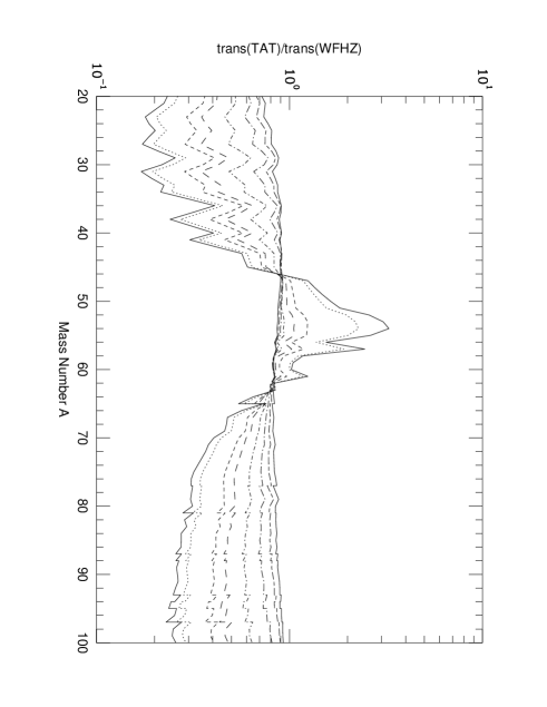
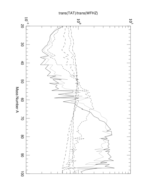
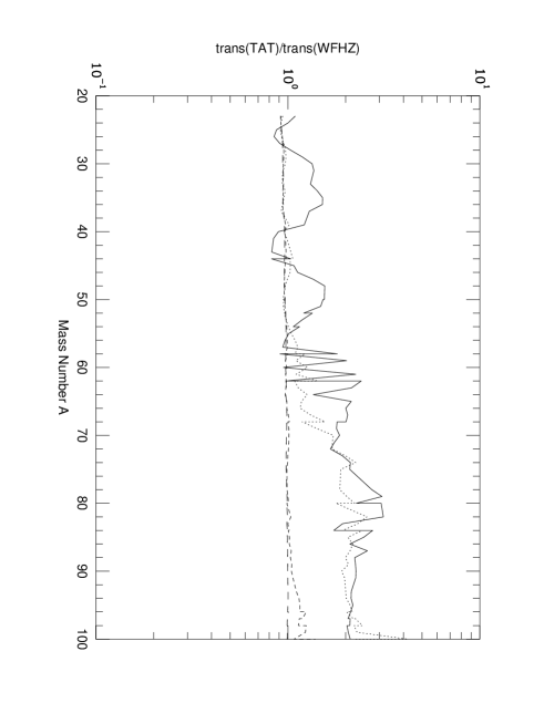
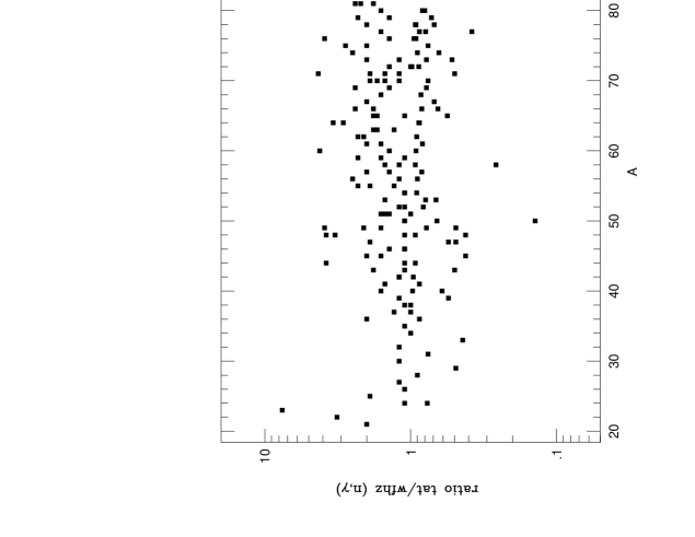
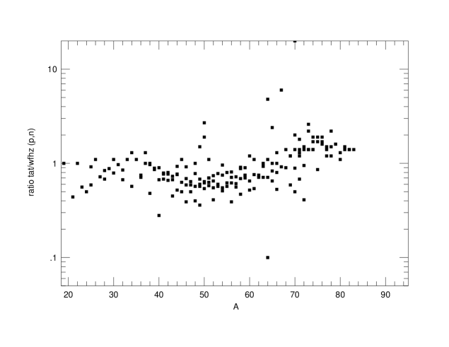
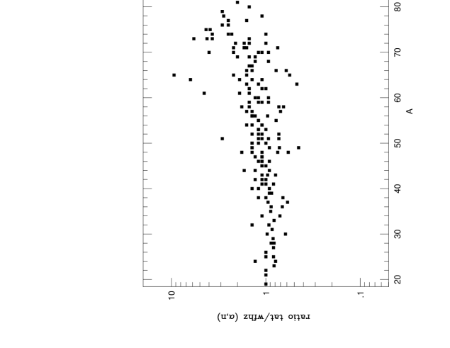
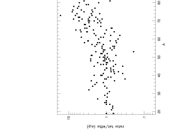


| Z | A | Amax | A | Amax | A | Amax |
|---|---|---|---|---|---|---|
| H | 1 | 3 | 1 | 3 | 1 | 3 |
| He | 3 | 4 | 3 | 4 | 3 | 4 |
| Li | 6 | 8 | 6 | 8 | 6 | 8 |
| Be | 7 | 9 | 7 | 9 | 7 | 10 |
| B | 8 | 11 | 8 | 11 | 10 | 12 |
| C | 11 | 14 | 11 | 14 | 11 | 14 |
| N | 13 | 15 | 13 | 15 | 13 | 17 |
| O | 15 | 18 | 15 | 18 | 14 | 20 |
| F | 17 | 20 | 17 | 19 | 17 | 21 |
| Ne | 19 | 23 | 19 | 23 | 18 | 25 |
| Na | 21 | 25 | 22 | 24 | 21 | 26 |
| Mg | 23 | 28 | 23 | 27 | 22 | 28 |
| Al | 25 | 30 | 25 | 28 | 24 | 30 |
| Si | 27 | 32 | 27 | 32 | 26 | 33 |
| P | 29 | 34 | 29 | 34 | 27 | 35 |
| S | 31 | 38 | 31 | 37 | 29 | 38 |
| Cl | 33 | 41 | 33 | 38 | 31 | 39 |
| Ar | 36 | 44 | 36 | 41 | 33 | 44 |
| K | 37 | 46 | 37 | 42 | 35 | 46 |
| Ca | 40 | 50 | 40 | 49 | 37 | 49 |
| Sc | 41 | 51 | 41 | 50 | 40 | 50 |
| Ti | 43 | 52 | 44 | 51 | 42 | 52 |
| V | 45 | 54 | 45 | 52 | 44 | 54 |
| Cr | 47 | 56 | 48 | 55 | 46 | 56 |
| Mn | 49 | 59 | 51 | 57 | 48 | 58 |
| Fe | 51 | 64 | 52 | 61 | 50 | 62 |
| Co | 54 | 65 | 55 | 62 | 52 | 63 |
| Ni | 55 | 68 | 56 | 65 | 54 | 67 |
| Cu | 57 | 71 | 57 | 66 | 57 | 69 |
| Zn | 59 | 74 | 60 | 69 | 59 | 72 |
| Ga | 61 | 77 | 61 | 70 | 61 | 74 |
| Ge | 64 | 80 | 64 | 71 | 63 | 78 |
| As | 66 | 83 | - | - | - | - |
| Se | 68 | 86 | - | - | - | - |
| Br | 70 | 89 | - | - | - | - |
| Kr | 72 | 90 | - | - | - | - |
| aafootnotetext: This study. bbfootnotetext: Woosley & Weaver 1995. ccfootnotetext: Thielemann, Nomoto, & Hashimoto, 1996. |
l c c c c c l \tablewidth0pt \tablecaption15 M⊙ Stellar Yields (in M⊙) 12C()=2.35*CF88 \tablehead \colheadAZ& \colheadWFHZ \colheadTAT \colheadWFHZ/TAT \colheadTNH \colheadTNH/TAT \colheadprocess(es)a \startdata1H & 6.96 6.96 1.00 — — BB\nl4He 5.21 5.21 1.00 1.83 0.351 BB,L*,H\nl12C 1.38(-1) 1.36(-1) 1.01 8.33(-2) 0.611 L*,He\nl14N 5.27(-2) 5.27(-2) 1.00 5.37(-3) 0.102 L*,H\nl16O 6.31(-1) 6.35(-1) 0.99 4.23(-1) 0.666 He\nl18O 6.06(-3) 6.06(-3) 1.00 1.35(-2) 2.228 He\nl19F 6.38(-6) 6.39(-6) 1.00 2.67(-11) — ,He\nl20Ne 2.60(-2) 2.57(-2) 1.01 2.83(-2) 1.102 C\nl21Ne 1.11(-4) 1.09(-4) 1.02 4.53(-5) 0.416 C\nl22Ne 7.48(-3) 7.52(-3) 1.00 1.26(-2) 1.676 He\nl23Na 1.02(-3) 1.03(-3) 0.99 2.09(-4) 0.202 C,Ne,H\nl24Mg 1.03(-2) 1.21(-2) 0.85 4.20(-2) 3.483 C,Ne\nl25Mg 1.91(-3) 1.92(-3) 1.00 3.46(-3) 1.803 C,Ne\nl26Mg 2.68(-3) 2.67(-3) 1.00 2.52(-3) 0.945 C,Ne\nl27Al 1.33(-3) 1.39(-3) 0.95 5.55(-3) 3.999 C,Ne\nl28Si 1.93(-1) 1.70(-1) 1.14 6.52(-2) 0.384 xO,O\nl29Si 1.16(-3) 1.22(-3) 0.95 4.40(-3) 3.615 C,Ne\nl30Si 6.05(-4) 5.92(-4) 1.02 4.91(-3) 8.326 C,Ne\nl31P 1.06(-3) 9.79(-4) 1.08 8.67(-4) 0.886 C,Ne\nl32S 1.65(-1) 1.84(-1) 0.90 2.16(-2) 0.117 xO,O\nl33S 1.18(-3) 1.60(-3) 0.74 9.31(-5) 0.058 xO,xNe\nl34S 7.70(-3) 8.65(-3) 0.89 1.09(-3) 0.126 xO,O\nl36S 3.22(-6) 3.14(-6) 1.03 5.27(-7) 0.168 He(s),C,Ne\nl35Cl 1.15(-3) 8.83(-4) 1.30 5.46(-5) 0.062 He(s),xO,xNe,\nl37Cl 3.38(-4) 4.17(-4) 0.81 5.62(-6) 0.013 xO,xNe\nl36Ar 4.71(-2) 4.73(-2) 1.00 3.49(-3) 0.074 xO,O\nl38Ar 1.39(-2) 1.54(-2) 0.90 3.26(-4) 0.021 xO,O\nl40Ar 1.11(-6) 9.58(-7) 1.16 4.12(-9) 0.004 He(s),C,Ne\nl39K 1.68(-3) 1.18(-3) 1.41 1.62(-5) 0.014 xO,O,\nl40K 2.24(-6) 1.73(-6) 1.30 7.04(-9) 0.004 He(s),C,Ne\nl41K 2.45(-4) 2.49(-4) 0.98 1.25(-6) 0.005 xO\nl40Ca 4.00(-2) 3.84(-2) 1.04 3.03(-3) 0.079 xO,O\nl42Ca 7.63(-4) 6.93(-4) 1.10 6.98(-6) 0.010 xO\nl43Ca 9.37(-6) 8.47(-6) 1.11 1.21(-6) 0.143 C,Ne\nl44Ca 8.00(-5) 9.36(-5) 0.86 7.19(-5) 0.768 ,Ia-det\nl46Ca 7.38(-8) 1.21(-7) 0.61 8.50(-12) — He(s),C,Ne\nl48Ca 1.75(-6) 1.75(-6) 1.00 6.71(-16) — nse-Ia-MCh\nl45Sc 3.55(-6) 2.91(-6) 1.22 4.66(-8) 0.016 ,xO,xSi,C,Ne,\nl46Ti 1.81(-4) 1.90(-4) 0.95 2.72(-6) 0.014 xO,Ia-det\nl47Ti 1.02(-5) 1.08(-5) 0.94 4.67(-6) 0.432 xO,xSi,Ia-det\nl48Ti 1.56(-4) 1.72(-4) 0.91 1.27(-4) 0.738 xSi,Ia-det\nl49Ti 1.49(-5) 1.18(-5) 1.26 4.15(-6) 0.352 xSi\nl50Ti 2.77(-6) 2.83(-6) 0.98 4.59(-10) — nse-Ia-MCh\nl50V 1.06(-7) 1.34(-7) 0.79 3.51(-10) 0.003 C,Ne,xNe,xO\nl51V 4.36(-5) 5.90(-5) 0.74 1.01(-5) 0.171 ,Ia-det,xSi,xO,\nl50Cr 2.31(-4) 2.83(-4) 0.81 3.85(-5) 0.136 xSi,xO,,Ia-det\nl52Cr 1.37(-3) 1.43(-3) 0.96 8.24(-4) 0.576 xSi,,Ia-det\nl53Cr 1.70(-4) 1.83(-4) 0.93 8.92(-5) 0.487 xO,xSi\nl54Cr 8.08(-6) 8.06(-6) 1.00 1.11(-10) — nse-Ia-MCh\nl55Mn 1.12(-3) 1.11(-3) 1.00 3.39(-4) 0.305 Ia,xSi,\nl54Fe 6.94(-3) 7.31(-3) 0.95 3.51(-3) 0.480 Ia,xSi\nl56Fe 9.65(-2) 9.61(-2) 1.00 1.30(-1) 1.353 xSi,Ia\nl57Fe 3.45(-3) 3.44(-3) 1.00 4.64(-3) 1.349 xSi,Ia\nl58Fe 1.58(-4) 1.60(-4) 0.99 3.82(-10) — He(s),nse-Ia-MCh\nl59Co 3.00(-4) 2.81(-4) 1.07 1.36(-4) 0.484 He(s),,Ia,\nl58Ni 4.22(-3) 4.34(-3) 0.97 6.64(-3) 1.529 \nl60Ni 2.50(-3) 2.67(-3) 0.94 3.13(-3) 1.172 ,He(s)\nl61Ni 1.52(-4) 1.49(-4) 1.02 1.46(-4) 0.980 ,Ia-det,He(s)\nl62Ni 7.11(-4) 8.91(-4) 0.80 1.00(-3) 1.122 ,He(s)\nl64Ni 4.36(-5) 4.59(-5) 0.95 9.17(-16) — He(s) \nl63Cu 4.01(-5) 3.16(-5) 1.27 9.56(-7) 0.030 C,Ne\nl65Cu 1.27(-5) 1.42(-5) 0.89 7.69(-7) 0.054 He(s)\nl64Zn 2.84(-5) 2.67(-5) 1.06 1.41(-5) 0.528 -wind,,He(s)\nl66Zn 5.56(-5) 5.78(-5) 0.96 1.47(-5) 0.254 He(s),,nse-Ia-MCh\nl67Zn 3.27(-6) 3.54(-6) 0.92 1.94(-8) 0.005 He(s)\nl68Zn 1.63(-5) 1.75(-5) 0.93 6.35(-9) — He(s)\nl70Zn 2.81(-7) 3.12(-7) 0.90 3.19(-21) — He(s)\nl69Ga 2.35(-6) 2.23(-6) 1.05 6.47(-13) — He(s)\nl71Ga 1.21(-6) 1.30(-6) 0.93 2.29(-20) — He(s)\nl70Ge 7.32(-6) 5.53(-6) 1.32 5.13(-15) — He(s)\nl\tablenotetextaNucleosynthetic process(es) responsible for the production where “BB” stands for the big bang (e.g. Walker et al. 1991); “L*” stands for low-mass stars (M M⊙ e.g. Renzini & Voli 1981) or in some cases AGB stars (Sackmann & Boothroyd 1992); “” is the neutrino process (e.g. Woosley et al. 1990); “-wind is the neutrino-driven wind from young neutron stars in Type II and Ib supernovae (e.g. Hoffman, Woosley, & Qian 1997); “” is the -rich freeze out from nuclear statistical equilibrium (e.g. Woosley, Arnett, & Clayton 1973); “Novae” indicates classical novae (e.g. Woosley 1986); “Ia” is Type Ia supernovae (Nomoto, Thielemann, & Yokoi 1984 for ordinary Ia’s which are assumed to ignite at the Chandrasekhar mass; Woosley & Eastman 1995 for the inner neutron-rich regions of ordinary Ia’s- here called “nse-Ia-MCh”; Woosley & Weaver 1994 for sub-Chandrasekhar detonation models “Ia-He-det”). All other entries refer to burning processes in massive stars, H, He, C, Ne, O, Si- responsible for producing the isotope, with a prefix “x” indicating explosive nucleosynthesis. \enddata
l c c c c c l \tablewidth0pt \tablecaptionRadioactive Stellar Yields (in M⊙) in the 15 M⊙Supernovae \tablehead \colheadAZ& \colheadWFHZ \colheadTAT \colheadWFHZ/TAT \colheadTNH \colheadTNH/TAT \colheadprocess(es)a \startdata22Na & 8.10(-8) 9.68(-8) 0.84 3.98(-8) 0.411 Novae\nl26Al 3.07(-5) 2.92(-5) 1.05 2.68(-6) 0.092 ,xNe,H\nl44Ti 6.06(-5) 7.40(-5) 0.82 7.19(-5) 0.972 \nl56Ni 8.11(-2) 8.06(-2) 1.01 1.30(-1) 1.613 ,nse-Ia-MCh\nl60Fe 3.35(-6) 5.51(-6) 0.61 1.25(-17) — Ne,xNe,xHe\nl60Co 5.63(-6) 2.60(-6) 2.17 4.14(-14) — Ne,xNe,xHe\nl\tablenotetextasee footnote table The Reaction Rate Sensitivity of Nucleosynthesis in Type II Supernovae \enddata
l c c c c c \tablewidth0pt \tablecaptionStatistical Errors of Reaction Ratios \tablehead \colhead()& \colhead# \colheadx̄WFHZ \colhead \colheadx̄TAT \colhead \startdata(n,)& 62 0.91 0.58 1.08 0.64\nl(p,n) 12 1.47 0.62 0.95 0.47\nl(p,) 20 1.35 0.81 1.33 0.65\nl(,p) 12 0.81 0.35 0.73 0.45\nl(,n) 16 0.85 0.39 0.86 0.23\nl(,) 2 1.10 0.36 1.25 0.25\nl\tablenotetextax̄ and indicate the arithmetic mean and standard deviation for the stated number (#) of cross section [(n,)] and reaction rate (all other channel) ratios (theory/experiment). \enddata
l c c c c c \tablewidth0pt \tablecaptionComparison of stellar reaction rates in cm3 s-1 mole-1 from the WFHZ, TAT, and NON-SMOKER reaction rate libraries. \tablehead \colheadReaction& \colhead \colheadWFHZ \colheadTAT \colheadTAT/WFHZ \colheadNON-SMOKER \startdata32S(n,)33Sa& 3.5 5.4(5) 6.9(5) 1.28 8.4(5)\nl33S(p,)34Cl 3.5 5.6(3) 1.1(4) 1.96 6.2(3)\nl33S(n,)30Si 3.5 5.1(7) 3.4(7) 0.67 3.4(7)\nl39K(n,)40Ka 1.0 1.4(6) 1.7(6) 1.21 1.8(6)\nl40K(n,)37Cl 1.0 1.1(7) 8.5(6) 0.77 7.6(6)\nl40K(n,p)40Ar 1.0 4.5(6) 1.8(6) 0.40 1.8(6)\nl45Ca(n,)46Ca 1.0 1.6(6) 2.5(6) 1.56 1.7(6)\nl46Ca(n,)47Caa 1.0 7.8(5) 7.9(5) 1.01 4.7(5)\nl44Ti(,p)47V 2.59.2(-3)9.6(-3) 1.049.6(-3)\nl45Ti(n,)42Ca 3.5 6.4(6) 9.9(6) 1.55 1.0(7)\nl45Ti(n,p)45Sc 3.5 1.7(8) 2.4(8) 1.41 2.5(8)\nl43Ca(p,)44Sc 3.5 3.9(4) 3.5(4) 0.90 3.2(4)\nl44Sc(p,)45Ti 3.5 1.2(4) 2.5(4) 2.08 1.6(4)\nl50V(n,)51V 3.5 2.8(6) 2.1(6) 0.75 3.9(6)\nl69Zn(n,)70Zn 1.0 6.6(6) 1.3(7) 1.97 1.1(7)\nl70Zn(n,)71Zn 1.0 1.4(6) 2.4(6) 1.71 2.6(6)\nl\tablenotetextaActual rate used by TAT and WFHZ is based on Bao & Käppeler 1987 \enddata
l c c c c c \tablewidth0pt \tablecaptionComparison of stellar () reaction rates (in cm3 s-1 mole-1) on self-conjugate nuclei derived from the CRSEC, SMOKER, and NON-SMOKER statistical model codes. \tablehead \colheadReaction& \colhead \colheadCRSEC \colheadSMOKER \colheadSM/CR \colheadNON-SMOKER \startdata24Mg()28Si& 2.5 1.1(1) 3.7(1) 3.36 2.8(0)\nl28Si()32S 2.5 3.8(-1) 4.5(0) 11.71 4.6(-1)\nl32S()36Ar 2.5 2.3(-1) 8.9(-1) 3.87 9.4(-2)\nl36Ar()40Ca 2.5 3.4(-3) 2.4(-2) 7.06 1.6(-3)\nl40Ca()44Ti 2.5 1.5(-2) 7.8(-2) 5.70 3.3(-3)\nl44Ti()48Cr 2.5 3.3(-6) 1.6(-4) 48.48 1.8(-5)\nl\enddata