Gravitational force distribution in fractal structures

Abstract

We study the (newtonian) gravitational force distribution arising from a fractal set of sources. We show that, in the case of real structures in finite samples, an important role is played by morphological properties and finite size effects. For dimensions smaller than $d-1$ (being $d$ the space dimension) the convergence of the net gravitational force is assured by the fast decaying of the density, while for fractal dimension $D>d-1$ the morphological properties of the structure determine the eventual convergence of the force as a function of distance. We clarify the role played by the cut-offs of the distribution. Some cosmological implications are discussed.

The aim of the present paper is to discuss the general properties of the gravitational field generated by a finite fractal distribution of field sources. This problem is nowadays particularly relevant. In fact, there is a general agreement that galaxy distribution exhibits fractal behavior up to a certain scale [1, 2]. The eventual presence of a transition scale towards homogeneity and the exact value of the fractal dimension are still matters of debate [3, 5, 4]. Moreover it has been observed that cold gas clouds of the interstellar medium have a fractal structure, with $1.5\leq D\leq 2$ in a large range of length scales [6]. For this case the general belief is that the origin of their fractality lies in turbulence. However recently [7] it has been pointed out that self-gravity itself may be the dominant factor in making clouds fractal.

Chandrasekhar [8], has considered the behavior of the newtonian gravitational force probability density arising from a poissonian distribution of sources (stars). In this case, in evaluating the probability distribution of the force acting on a particle, one supposes that fluctuations are subject to the restriction that a constant average density occurs, i.e. the source distribution is spatially homogeneous and the density fluctuations obey to the Poisson statistics. Applying the Markov’s method, it is possible to compute explicitly the force probability density, known as the Holtsmark’s distribution. In this case, the probability density of the force $F$ is given by

$$W(F)=\frac{H(\beta)}{F_{o}}$$ (1)

where $F_{o}=(4/15)^{2/3}(2\pi GM)n^{2/3}$ is the normalizing force ($n$ is the average density of sources, $M$ is the mass of each punctual source and $G$ is the gravitational constant), $\beta=F/F_{o}$ is an adimensional force and

$$H(\beta)=\frac{2}{\pi\beta}\int_{0}^{\infty}dx\;\exp[-(x/\beta)^{\frac{3}{2}}]\;x\;\sin(x)\;.$$ (2)

The main result is that, in the thermodynamic limit ($V\rightarrow\infty$ with $n$ constant), the force distribution has a finite first moment and an infinite variance. This divergence is due to the possibility of having two field sources arbitrarily nearby. The approximate solution given by the nearest neighbor (n.n.) approximation (i.e. by considering only the effect of the n.n. particle) and the exact Holtsmark’s distribution (Eq.2) agrees over most of range of $F$ (see Fig.1). The region where they differ mostly is when $F\rightarrow 0$. This is due to the fact that a weak field arises from a more or less symmetrical distribution of points, and hence the n.n. approximation fails. Therefore in the strong field limit we may neglect the contribution to the force of far away points, because the main contribution is due to $r\rightarrow 0$ (i.e. it comes from the n.n). The root mean square of the force is divergent as in the case of the n.n. approximation, and this is due to the fact that the limit $r\rightarrow 0$ is allowed. If there exists a lower cut-off (see below) this divergence is erased out. However, due to isotropy, no divergence problem arises from the faraway sources even in the limit $r\rightarrow\infty$.

The derivation of Chandrasekhar cannot be easily extended to the case of fractal distributions because, in such structures, fluctuations are characterized by long-range correlations. A fractal is an instrisic critical structure characterized by self-similarity. The scale-invariant properties of such distributions are described by slow power law decreasing density-density correlation functions whose exponents are the main characteristic quantities to be studied (see [9] and [1]). In this situation an analytic treatment of the force distribution becomes very difficult. Vlad [10] developed a functional integral approach for evaluating the stochastic properties of vectorial additive random fields generated by a variable number of point sources obeying to inhomogeneous Poisson statistics. Then he applied these results to the case of the gravitational force generated by a fractal distribution of field sources under some strong approximations. In particular, in order to compute analytically the force probability density, Vlad [10] has not considered the presence of intrinsical fluctuations in the space density. In fact, in the computation of the density from a single point one expects to see deviation from the average scaling behavior, which are present at any scale (see below). Such a situation occurs in any real fractal structure and can be quantified by studying the $n$-point correlation functions [11]. Instead, the derivation has been done under the assumption that the $n+1$-point correlation function (where the $(n+1)^{th}$ point is the occupied origin) can be written as $g(\vec{x_{1}},\vec{x_{2}},...,\vec{x_{n}})\propto g(\vec{x_{1}})g(\vec{x_{2}})...g(\vec{x_{n}})\;,$where $g(\vec{x})$ is the two-point correlation function. Such an approximation is not adequate to describe the effect of morphology and hence in real cases the situation is quite different. Instead of Eq.2, Vlad found that the probability density of the absolute value $F$ (generalized Holtsmark’s distribution) of the field intensity is equal to

$$H(\beta,D)=\frac{2}{\pi\beta}\int_{0}^{\infty}dx\;\exp[-(x/\beta)^{\frac{D}{2}}]\;x\;\sin(x)\;.$$ (3)

In this case $F_{o}=(4/15)^{2/D}(2\pi GM)(DB/(4\pi))^{2/D}$, where $B$ is a constant characterizing the average mass in the unitary sphere and $\beta=F/F_{o}$. The main change due to the fractal structure is that the scaling exponent in Eq.3 is $D/2$ rather than $3/2$. Hence in this case the tail of the probability density has a slower decay than in the homogeneous case (see Fig.1). This means that the variance of the force is larger for $D<3$ than for the $D=3$. As we discuss below, the case $D<2$ is rather well described by Eq.3: this is not the case for $D>2$ where the $n-th$ points correlations must be taken into account in the case of real structures. An important limit is the strong field one ($F\rightarrow\infty$). In this case it is possible to show that the force distribution of Eq.3 can be reduced to the one derived under the n.n. approximations:

$$W_{nn}(F)dF=\frac{DB}{2}(GM)^{\frac{D}{2}}F^{-\frac{D+2}{2}}\\ \exp\left(-B(GM)^{\frac{D}{2}}F^{-\frac{D}{2}}\right)dF\;.$$ (4)

The n.n. approximation is good for $F\gg F_{1}$, where $F_{1}=\left(B\right)^{\frac{2}{D}}\cdot GM$. From Eq.4, in the fractal case, as in the homogeneous one, the divergences of the force moments (the second for $D\leq 3$ and the first for $D\leq 2$) are due only to the fact that two field sources can be arbitrarily close. If we impose that a lower cut-off $\Lambda>0$ (minimal distance between the sources) exists, these divergences are erased out. According to the approximations previously mentioned, far away points do not produce any divergence neither in the average force nor in its variance. This is related to the fact that if the volume involved is large enough with respect to $\Lambda$ the distribution becomes spherically symmetric in a statistical sense and the anisotropies become negligible.

In the n.n. approximation (Eq.4), we obtain for the average force $\left\langle F\right\rangle\sim(1/\Lambda)^{2-D}$. Hence in the limit $\Lambda\rightarrow 0$, $\left\langle F\right\rangle$ is finite for $D>2$, while it is infinite for $D<2$. The force r.m.s value can be computed in the same way and we readily obtain $\left\langle F^{2}\right\rangle\sim(1/\Lambda)^{4-D}$ so that, in the limit $\Lambda\rightarrow 0$, $\left\langle F^{2}\right\rangle$ is divergent for any possible value of the fractal dimension such that $D\leq 3$. Therefore the r.m.s. value of the force strongly depends on the lower cut-off $\Lambda$. Consequently, in this context, we expect to see large fluctuations from the average value changing the origin point on different masses in the sample. This kind of divergence is due to the fact that there is no restriction on the distance $\Delta r$ between two neighbor field sources, i.e. we may have $\Delta r\rightarrow 0$. To assume $\Lambda>0$ is quite reasonable for almost every physical problem and in particular for the case of galaxy distribution. In fact, if two galaxies were too close, they should be subjected to tidal interactions and then should form a binary system. Such a situation goes beyond the scope of this paper.

As we have already mentioned, the Vlad’s result has been obtained under an assumption which is equivalent to the condition that the mass-length relation (m.l.r.) $N(<r)$ from a single point is exactly a power law function:

$$N(<r;\hat{\phi},\Omega)=B\frac{\Omega}{4\pi}r^{D}\;.$$ (5)

Eq.5 gives the mass contained in a portion of a sphere of radius $r$, being a generic fixed point at the origin, which covers a solid angle $\Omega$ in the direction $\hat{\phi}$. From this equation we can derive directly the number density in the same volume by dividing it for the volume itself (in $d=3$)

$$n(<r;\hat{\phi},\Omega)=\frac{B}{4\pi}r^{D-3}$$ (6)

It is important to notice, instead, that the m.l.r. has a genuine power law behavior only when it is averaged over all the points $\vec{x}$ of the structure, obtaining the so-called two-point correlation function (tpcf). From a single point there can be important intrinsical fluctuations around the power law behavior [11]. In fact, since a fractal is an intrinsically critical system with strong correlations on all scales, we expect that the density from one point shows large fluctuations, with respect to the tpcf, changing $r$ with fixed $\hat{\phi}$ or vice-versa. In general these intrinsic fluctuations can be characterized as log-periodic corrections to scaling [11]. These fluctuations can be present at any scale (i.e. whatever is $r$) and they can be angularly correlated, that is the quantity

$$dn(|\hat{\phi}_{1}-\hat{\phi}_{2}|;r)=\left\langle(n(<r;\hat{\phi}_{1},\delta\Omega)-n(<r;\hat{\phi}_{2},\delta\Omega))^{2}\right\rangle$$ (7)

depends on the angular distance between $\hat{\phi}_{1}$ and $\hat{\phi}_{2}$. As we show below, these fluctuations can play a crucial role in the determination of the force distribution. In order to consider, in a simple way, the important effect of morphology, we study the r.m.s force for a generic random fractal distribution in the three dimensional Euclidean Space. We consider explicitly the existence of a minimal distance (i.e. lower cut-off) $\Lambda$ and a maximal distance (i.e. upper cut-off) $R_{s}$ from the origin, and then we derive the asymptotic behavior for $\Lambda\rightarrow 0$ and $R_{s}\rightarrow\infty$. Let $\vec{F}$ be the total force acting on a particle due to all the other field sources having the same unitary mass ($GM=1$). We consider the contribution to the force by all the field sources in the spherical shell $[\Lambda,R_{s}]$

$$\vec{F}(\Lambda,R_{s})=\sum_{\Lambda\leq|\vec{r}_{i}|\leq R_{s}}^{i=1,N}\frac{\vec{r}_{i}}{r_{i}^{3}}$$ (8)

where $N$ is the total number of the sources in the shell considered and $\vec{r}_{i}$ is the position of the $i-th$ source with respect to the one in the origin. Under the assumption that the mass distribution is statistically isotropic, we have

$$\lim_{R_{s}/\Lambda\rightarrow\infty}\left|\left\langle\vec{F}(\Lambda,R_{s})\right\rangle\right|=0\;.$$ (9)

The statistical average of the force square modulus is given by:

$$\left\langle|\vec{F}(\Lambda,R_{s})|^{2}\right\rangle=\left\langle F(\Lambda,R_{s})^{2}\right\rangle=\left\langle\sum_{\Lambda\leq|\vec{r}_{i}|\leq R_{s}}^{i=1,N}\frac{1}{r_{i}^{4}}\right\rangle+\left\langle\sum_{\Lambda\leq|\vec{r}_{i}|\leq R_{s}}^{i\neq j=1,N}\frac{\cos(\theta_{ij})}{r_{i}^{2}r_{j}^{2}}\right\rangle$$ (10)

where $\theta_{ij}$ is the angle formed by $\vec{r}_{i}$ and $\vec{r}_{j}$. Here the average $<...>$ is made over an ensemble of different realizations of the sample or, when this is not possible, over all the possible origins in a single sample. Obviously, the first term is simple to analyze, while the second one deserves a more careful discussion because it involves the three-point correlation function. The first term can be written as

$$\left\langle\sum_{\Lambda\leq|\vec{r}_{i}|\leq R_{s}}^{i=1,N}\frac{1}{r_{i}^{4}}\right\rangle=DB\int_{\Lambda}^{R_{s}}dr\frac{r^{D-1}}{r^{4}}=\frac{DB}{4-D}\frac{1}{\Lambda^{4-D}}\left(1-\left(\frac{\Lambda}{R_{s}}\right)^{4-D}\right)\;.$$ (11)

In Eq.11 we have considered that $<...>$ leaves only the power law behavior in the m.l.r. In fact we can write $\sum_{i=1}^{N}\frac{1}{r_{i}^{4}}=\int_{\Lambda,R_{s}}d^{3}rn(\vec{r})/r^{4}$, where $n(\vec{r})=\sum_{i=1}^{N}\delta(\vec{r}-\vec{r_{i}})$ is the number density, which can be different from a power law and show persistent fluctuations around its average behavior, and $<...>$ erases these fluctuations as well as the dependence from the direction of $\vec{r}$. Analogously, the second term in Eq.10 can be written as

$$\left\langle\sum_{\Lambda\leq|\vec{r}_{i}|\leq R_{s}}^{i\neq j=1,N}\frac{\cos(\theta_{ij})}{r_{i}^{2}r_{j}^{2}}\right\rangle=\int_{V}\int_{V}d^{3}r_{1}d^{3}r_{2}p(\vec{r}_{1},\vec{r}_{2})\frac{\cos(\theta_{12})}{r_{1}^{2}r_{2}^{2}}$$ (12)

where $p(\vec{r}_{1},\vec{r}_{2})d^{3}r_{1}d^{3}r_{2}$ is equal to $N(N-1)$ times the probability to have a particle in the infinitesimal volume $d^{3}r_{1}$ and, at the same time, another in the volume $d^{3}r_{2}$, i.e. the number of pairs in which the first particle is in $d^{3}r_{1}$ and the second in $d^{3}r_{2}$. The function $p(\vec{r}_{1},\vec{r}_{2})$ is strictly related to the three-point correlation function in which the first point is the origin and the others are $\vec{r}_{1}$ and $\vec{r}_{2}$. Such a function is usually very difficult to be computed for a generic fractal structure [11]. Note that $p(\vec{r}_{1},\vec{r}_{2})\sim\left\langle n(\vec{r}_{1},\vec{r}_{2})\right\rangle$ where $n(\vec{r}_{1},\vec{r}_{2})=\sum_{i,j}\delta(\vec{r_{i}}-\vec{r_{1}})\delta(\vec{r_{j}}-\vec{r_{2}})\;.$ We expect that $p(\vec{r}_{1},\vec{r}_{2})$ depends only on $r_{1}$ and $r_{2}$ and the angle $\theta$ between the two directions because of the average $<...>$. We make the following approximation, by using the tpcf and the angular correlation function

$$\int_{\theta\leq|\vec{\Omega}_{1}-\vec{\Omega}_{2}|\leq\theta+d\theta}p(\vec{r}_{1},\vec{r}_{2})d\Omega_{1}d\Omega_{2}\simeq(4\pi)^{2}\left\langle n(r_{1})\right\rangle\left\langle n(r_{2})\right\rangle\Gamma\left(\theta,\frac{r_{1}}{r_{2}}\right)d\theta$$ (13)

where $\Gamma(\theta,r_{1}/r_{2})$ is the probability that the angle between $\vec{r}_{1}$ and $\vec{r}_{2}$ is in the range $[\theta,\theta+d\theta]$, conditioned to the fact that the distances of the two sources are $r_{1}$ and $r_{2}$. The dependence of $\Gamma(\theta,r_{1}/r_{2})$ on the ratio $r_{1}/r_{2}$ is in general a peculiar property of the fractal studied. This problem has been studied in detail by [11]. In what follows, we neglect the dependence on the ratio $r_{1}/r_{2}$, which can be treated as a perturbation [11]. This approximation consists in substituting $\Gamma(\theta,r_{1}/r_{2})$ with the angular correlation function $\Gamma(\theta)$ normalized to unity. $\Gamma(\theta)$ is obtained by the analysis of the angular projection of the sample.

Under this approximation we can write Eq.12 as

$$\left\langle\sum_{\Lambda\leq|\vec{r}_{i}|\leq R_{s}}^{i\neq j=1,N}\frac{\cos(\theta_{ij})}{r_{i}^{2}r_{j}^{2}}\right\rangle=\frac{(DB)^{2}C(D)}{(2-D)^{2}}\frac{1}{\Lambda^{4-2D}}\left(1+\left(\frac{\Lambda}{R_{s}}\right)^{4-2D}-2\left(\frac{\Lambda}{R_{s}}\right)^{2-D}\right)$$ (14)

where $C(D)=\int_{0}^{\pi}\Gamma(\theta)\cos(\theta)d\theta\;.$ The presence of fluctuations in the m.l.r. from one point are crucial in determining the behavior of $\Gamma(\theta)$ and then the convergence properties of $\left\langle F^{2}\right\rangle$. To clarify this point, consider the quantity $dn(|\hat{\phi}_{1}-\hat{\phi}_{2}|;r)$ in Eq.7. It is simple to show analytically that this quantity is strictly related to $\Gamma(\theta)$ where $\theta=|\hat{\phi}_{1}-\hat{\phi}_{2}|$ is the angular distance between $\hat{\phi}_{1}$ and $\hat{\phi}_{2}$. At this point is convenient to distinguish the cases $D<2$ and $D\geq 2$. For $D<2$, even in absence of fluctuations in the m.l.r., we have $C(D)>0$ (the effect of fluctuations is only a change in the non-vanishing value of $C(D)$), while for $D\geq 2$, $C(D)>0$ only because of these fluctuations. In the latter case and in absence of fluctuations, one would have a case very similar to the homogeneous one [9] in which $\Gamma(\theta)$ is constant and therefore $C(D)=0$.

Consequently, for $D<2$, the leading behaviors of $\left\langle F^{2}\right\rangle$ are:

$$\left\{\begin{array}[]{ll}\left\langle F^{2}\right\rangle\simeq\alpha(B,D)\Lambda^{-(4-D)}&for\;\Lambda\rightarrow 0\\ &and\;R_{s}finite\\ \left\langle F^{2}\right\rangle\simeq F^{2}_{\infty}-2\beta(B,D)\left(\frac{\Lambda}{R_{s}}\right)^{2-D}&for\;\frac{R_{s}}{\Lambda}\rightarrow\infty\\ &and\;\Lambda>0\\ \end{array}\right.$$ (15)

In Eq.15, $\alpha(B,D)=BD/(4-D)$ , $\beta(B,D)=(DB)^{2}C(D)/[(2-D)^{2}\Lambda^{4-2D}$ and $F^{2}_{\infty}=\alpha(B,D)\Lambda^{-(4-D)}+\beta(B,D)$ is the finite asymptotic value of $\left\langle F^{2}\right\rangle$ for $R_{s}/\Lambda\rightarrow\infty$. Obviously for intermediate ranges of $R_{s}/\Lambda$, other powers of it in Eq.11 and Eq.14 are important.

The case $D>2$ is very different and the effect of eventual fluctuations in the m.l.r. from one point can be crucial for the convergence of $\left\langle F^{2}\right\rangle$ in the limit $R_{s}/\Lambda\rightarrow\infty$. As a first step let us suppose that the m.l.r. from one point is a pure power law. In this case the function $\Gamma(\theta)$ is expected to be a constant and then $C(D)=0$. As a consequence we have that the second term in Eq.10 is equal to zero and $\left\langle F^{2}\right\rangle$ is simply given by

$$\left\langle F^{2}\right\rangle=\frac{DB}{4-D}\frac{1}{\Lambda^{4-D}}\left(1-\left(\frac{\Lambda}{R_{s}}\right)^{4-D}\right)\;.$$ (16)

This quantity diverges for $\Lambda\rightarrow 0$ as $\Lambda^{-(4-D)}$ and for $\Lambda>0$ it converges for $R_{s}/\Lambda\rightarrow\infty$.

In the case in which fluctuations around the power-law relation in the m.l.r. are present (and this is the more general case), the behavior is more complex. In this case $\Gamma(\theta)$ is not anymore constant, since we expect that the effect of these fluctuations is to introduce some angular correlations at least at small angles. The reason is that these fluctuations are due to the sequence of voids and clusters of masses in a fractal sample. These sequences are not the same in different directions, but they are angularly correlated and the average $<...>$ does not erase these correlations. In such a case $\left\langle F^{2}\right\rangle$ is given by

$$\left\langle F^{2}\right\rangle=\frac{DB}{4-D}\frac{1}{\Lambda^{4-D}}\left(1-\left(\frac{\Lambda}{R_{s}}\right)^{4-D}\right)+\frac{(DB)^{2}C(D)}{(D-2)^{2}}\frac{1}{\Lambda^{4-2D}}\left(1+\left(\frac{R_{s}}{\Lambda}\right)^{2D-4}-2\left(\frac{R_{s}}{\Lambda}\right)^{D-2}\right)$$ (17)

From Eq.(17) we can see that, for $R_{s}$ finite, $\left\langle F^{2}\right\rangle$ diverges as $\Lambda^{-(4-D)}$ (as in the case $D<2$) when $\Lambda\rightarrow 0$, and for $\Lambda>0$ it diverges as $(R_{s}/\Lambda)^{2D-4}$ in the limit $R_{s}/\Lambda\rightarrow\infty$. This last behavior is in striking contrast with the Vlad’s one for the same values of $D$; this is due to the fact that as mentioned Vlad does not consider the fluctuations in the m.l.r. from a single point. At intermediate scales the behavior is more complex and depend on the values of the parameter $D$, $B$ and the value of $C(D)$.

We have tested the results obtained in Eq.20 by numerical simulations. We have generated artificial fractals by means of different algorithms: random cantor set, levy flight and random walk [9]. With these algorithms the fractal dimension can be tuned appropriately (i.e. the tpcf), while the morphological properties of the structure (and hence the higher order correlations) are determined by the kind of iterative process choosen. For this reason the simulations do not have the same morphology of real galaxy distribution. A more realistic study for the case of galaxy structures is in progress, and here we are concerned with a more general problem. The agreement with Eq.20 is rather good for both cases $D<2$ and $D>2$. We stress again that the divergence of Eq.20 as a function of $R_{s}$ is strictly related to the morphological properties of the structure considered.

The clarification of the properties of the gravitational field in fractal structures is particularly relevant for the studies of the matter distribution in the universe. It is commonly believed that the peculiar velocity field (derived as a distortion from a pure linear Hubble law) is generated by local matter inhomogeneities in the distribution of galaxies [12]. A standard hypothesis in this framework is that, on large enough scale, the linear perturbation theory holds, as density fluctuations are small enought, and by using such an approximation one may “reconstruct” the peculiar velocity field from the matter one or vice-versa. Clearly, if matter distribution shows fractal properties, the linear theory fails. A related problem consists in the computation of the net gravitational force, due to the local inhomogeneities of matter distribution, acting on our galaxy (the dipole) [12]. Here we have shown that the eventual convergence or divergence of the dipole is related to subtle morphological properties of the sources distribution and not only to the prtoperties of the tpcf. In the universe we observe an irregular distribution of galaxies characterized by fractal properties [1], and hence its relationship with the peculiar velocity field must be much more complex than the one expected in the linear theory [12]. Such a situation deserves further studies, and in this paper we have considered some basic problems related to it.

Acknowledgments We would like to warmly thank L. Pietronero and M. Montuori for useful comments and remarks. We also thank Y. Baryshev, H. de Vega, R. Durrer, M. Joyce and N. Sanchez for enlighting discussions. A.G. and F.S.L. acknowledge the support of the EEC TMR Network ”Fractal structures and self-organization” ERBFMRXCT980183.

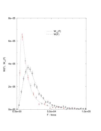
Fig. 1.–: (Upper panel) Force distribution due the n.n. (crosses) and due to all the field sources (diamonds) for an homogeneous sample with $n=N/V=2.39\cdot 10^{4}$ in $d=3$. The dotted line represents the force distribution $W(F)$ computed by the n.n. approximation, while the dashed line is the Holtsmark’s distribution (Eq.2). The agreement is quite satisfactory at strong field, and there is a deviation at weak field. (Bottom Panel) The same for a fractal with $D=1.98$ generated by a random walk in $d=3$. In this case we have used the generalized Holzmark distribution and its n.n. approximation for the fits (dotted and dashed lines)

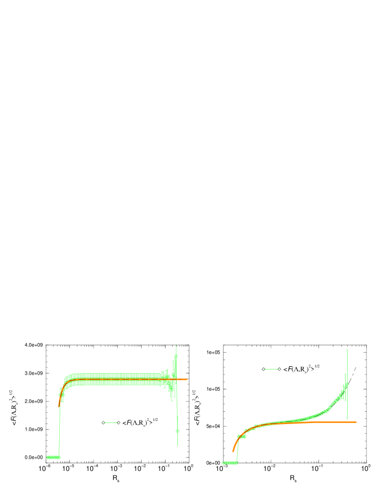
Fig. 2.–: (Left Panel) Behavior of $\sqrt{\langle F(\Lambda,R_{s})^{2}\rangle}$ as a function of $R_{s}$ for a fractal with $D=1.5$ generated by the random cantor set algorithm. The dashed line represents the first term in Eq.20, while the solid line both contributions in Eq.20. The agreement is rather good. (Right Panel) The same for a fractal with $D=2.7$. The effect of the angular correlations is now important and determine the divergence of $\sqrt{\langle F(\Lambda,R_{s})^{2}\rangle}$. The error bars have been computed over an average of 5 different realization of the same structure.

References

- [1] Sylos Labini F., Montuori M., Pietronero L., Phys.Rep. 293, 66 (1998); Coleman, P.H. & Pietronero, L., Phys.Rep. 231, 311 (1992)
- [2] Peebles P. J. E., “Principles of physical cosmology” (1993), Princeton Univ. Press
- [3] Davis, M., in the Proc. of the Conference ”Critical Dialogues in Cosmology” N. Turok Ed., p.13 (1997), World Scientific
- [4] Wu K.K.S., Lahav O. and Rees M., (1998) Nature In the press (astro-ph/9804062)
- [5] Pietronero, L., Montuori, M. and Sylos Labini, F., in the Proc of the Conference ”Critical Dialogues in Cosmology” N. Turok Ed., p.24 (1997), World Scientific
- [6] Larson R.B., Month.Not.R.acad.Soc. 194, 809 (1981) ; Scalo J.M., in Interstellar Medium eds Hollenbach D.J. & Thronson H.A., 349 (Reidel & Dorotech)
- [7] de Vega H.J., Sanchez N. , Combes F. Nature 383, 53 (1996); de Vega H.J., Sanchez N. , Combes F. Astrophysical Journal 500, 8 (1998)
- [8] Chandrasekhar S., Rev. Mod. Phys. 15, 1 (1943)
- [9] Mandelbrot, B.B., Fractals:Form, Chance and Dimension, W.H.Freedman, (1977)
- [10] Vlad M.O., Astrophysics and Space Science 218, 159 (1994)
- [11] Blumenfeld R. and Ball R.C., Phys. Rev E. 47, 2298 (1993)
- [12] Strauss M. and Willick Physics Reports 261 , 271 (1995)