Luminosity Distributions within Rich Clusters - II:
Demonstration and Verification via Simulation

Abstract

We present detailed simulations of long exposure CCD images. The simulations are used to explore the validity of the statistical method for reconstructing the luminosity distribution of galaxies within a rich cluster i.e. by the subtraction of field number-counts from those of a sight-line through the cluster. In particular we use the simulations to establish the reliability of our observational data presented in Paper 3. Based on our intended CCD field-of-view (6.5 by 6.5 arcmins) and a 1-$\sigma$ detection limit of 26 mags per sq arcsecond, we conclude that the luminosity distribution can be robustly determined over a wide range of absolute magnitude ($-23<M_{R}<-16$) provided:

(a) the cluster has an Abell richness 1.5 or greater,

(b) the cluster’s redshift lies in the range $0.1<z<0.3$,

(c) the seeing is better than FWHM 1.25^′′ and

(d) the photometric zero points are accurate to within $\Delta m=\pm 0.12$.

If these conditions are not met then the recovered luminosity distribution is unreliable and potentially grossly miss-leading. Finally although the method clearly has limitations, within these limitations the technique represents an extremely promising probe of galaxy evolution and environmental dependencies.

Keywords: galaxies: luminosity function, mass function - galaxies:evolution.

1 Introduction

In the first paper in this series (Smith, Driver & Phillipps 1997; hereafter Paper I), we compared the derived luminosity distributions (LD) of three rich clusters, A963 (Driver et al. 1994), A2554 (Paper I) and Coma (Bernstein et al. 1996), and postulated the existence of a ubiquitous dwarf-rich LD for rich clusters. This has had additional support from results published by other groups, in particular Wilson et al. (1997) who applied similar methods to recover the LDs in A1689 & A665, and found similar dwarf-rich LFs. These results are based on a statistical method which relies on the subtraction of galaxy number-counts detected in a non-cluster sight-line from those detected in a cluster sight-line. The observed number-count excess along the cluster’s sight-line is a direct representation of the cluster population. The method is observationally simple, requires minimal telescope time, yet provides a direct measurement of the fundamental luminosity density-distribution of galaxies within that cluster. This is only otherwise achievable via a time-intensive spectroscopic survey. Furthermore, even if telescope time limitations are neglected, spectroscopic surveys can only probe to low luminosity levels in nearby groups (e.g. de Propris et al. 1995) and nearby clusters (see for example Bernstein et al. 1996; and Bivanio et al. 1996). To assemble a sufficiently large number of measurements of the luminosity distribution of galaxies over a range of environments and epochs a statistical approach is required. This is the goal of these next two papers in the series, published here back-to-back. In this paper (Paper II), we first fully assess the accuracy, limitations and the presence of any systematic dependencies in the method via extensive and realistic simulations. In the following paper (Driver, Couch & Phillipps 1998; hereafter Paper III), we present new measurements of the LD for a sample of 7 rich clusters, armed with a very firm understanding of the characteristics and quality of these data from our simulations.

The plan of this paper is as follows: In §2 we describe in detail the process of simulating individual galaxies, the range of types, the magnitude-density calculation and the simulation of noise processes. In §3 we discuss our chosen photometry package (SExtractor, Bertin & Arnout 1996). In §4 we carry out our simulation of galaxy clusters and in §5 we run extensive simulations to explore the reliability of the technique and the range of observable parameters over which our LD recovery technique is valid. The final section (§6) contains an overall summary of our findings.

2 The Simulation Process

The principal aim of the simulation software is to adopt the main aspects of galaxy parameterisation to generate realistic deep CCD images. Below we define our adopted generic types, our method for the determination of the line-of-sight number counts for each type, and the process of simulation.

2.1 Simulated morphological types

To create a realistic CCD image we adopt four basic generic galaxy types selected to span the range from well ordered early systems to asymmetrical late systems. These types are: Ellipticals (E), spirals (Sb), irregulars (Irr) and dwarf ellipticals (dE). The field LFs and luminosity-surface brightness relations for these types are taken from Marzke et al. (1995) and Binggeli (1994) respectively (c.f. Table 1). In addition to the four generic galaxy types, stars are also simulated. The details of each generic type are as follows (see also Table 1) :

Ellipticals: These are assumed to exhibit $r^{\frac{1}{4}}$ de Vaucouleurs (1959) light profiles. Their ellipticity (or $(a-b)/a$, where $a$ and $b$ are the major and minor axis), is randomly distributed within the range 0.0 to 0.7 (i.e. E0—E7 in conventional nomenclature) with equal probability. The light-profile is simulated out to $\sim 6$ half-light radii.

Spirals: The majority of the total flux (75%) is simulated as a perfect exponential disk (Freeman 1970) with inclination in the range 0—90 degrees. The remaining 25% of flux is placed in a centrally located bulge (profiled as an elliptical galaxy as discussed above). This bulge-to-disk ratio is consistent with a stage 3 galaxy (Sb) on the 14 step revised Hubble classification scheme (Simien & de Vaucouleurs 1986). The inclination angle ($i$) and position angle (PA) of the disk are randomly generated with equal probability. The ellipticity is derived from the inclination ($i$) and intrinsic axis ratio ($Q_{o}$) as follows (c.f. Hubble 1926):

$$\cos^{2}(i)=\frac{(\frac{a}{b})^{2}-Q_{o}^{2}}{1-Q_{o}^{2}}$$ (1)

where, $Q_{o}$, the intrinsic axis ratio, is taken as 0.2 (c.f. Holmberg 1946). The disk is profiled out to 10 scale-lengths. Galaxy disks are treated as optically thin, and therefore the simulated galaxy’s total magnitude remains independent of inclination (but surface brightness does not).

Irregulars: The irregulars are modeled on a disk system containing a number of active star-forming regions. To achieve this 20% to 50% of the total luminosity is distributed as an exponential disk, identical to the mid-type spirals. The remaining flux is randomly distributed within three scale lengths across the primary disk as secondary superimposed mini-disks. An intrinsic disk axis ratio of $Q_{o}$ = 0.4 is adopted, implying a minimally rotating thick disk. Each simulated HII complex contains 5% of the total integrated flux. The central surface brightness of these HII complexes is randomized over a range of 2 mags arcsec^-2 about the central surface brightness of the underlying disk.

Dwarf Ellipticals: These systems are numerous within cluster environments (c.f. Ferguson & Binggeli 1994) and are simulated here as perfect exponential disks with no bulge or irregularity. An intrinsic disk axis ratio of $Q_{o}$ = 0.7 is adopted to reflect the lack of strong dynamical rotation and the probable tri-axial nature of these systems.

Stars: These are added after convolution with the Gaussian seeing disk and are simulated as a pure Gaussian profile, i.e. the diffraction rings of the Airy disk are neglected. For those stars with excessive flux, this excess is redistributed into two diffraction spikes aligned along the axis of the frame edges and a general low surface brightness “halo” is superimposed. The intention is to create a more realistic image rather than accurate treatment of bright stars, as few will be simulated per field of view and, at these magnitudes, the star/galaxy separation is trivial. Typically in the simulations described here the “diffraction spiking” occurs at magnitudes of $m_{R}<18.5$.

2.2 Simulating a field sight-line

To generate a simulated field sight-line we adopt the numerical morphological number-count model of Driver et al. (1995). This model is based on the following: an observed field luminosity function for each galaxy type (c.f. Marzke et al. 1995), the visibility—distance relationships for a standard flat cosmology (c.f. Phillipps, Davies & Disney 1990), K-corrections based on data from Pence (1976); King & Ellis (1985) and the observed luminosity—surface brightness relationships for each of the four adopted galaxy types (taken from the schematic of Binggeli 1994). The exact values used are summarized in Table 1 and more extensive details with regards the generation of differential galaxy number-counts are described in Driver et al. (1994); Driver, Windhorst & Griffiths (1995) and Driver et al. (1995). The only adjustable parameters in this prescription are the normalisation of the individual luminosity functions, and these have been optimised such that our simulated morphological number-counts match those observed in the Hubble Deep Field (c.f. Williams et al. 1996 and other deep Hubble Space Telescope WFPC2 images (c.f. Odewahn et al. 1996).

To allow for field-to-field variation the final numbers of each galaxy type at each magnitude interval are adjusted to reflect Poisson counting statistics. In those cases where less than one object is predicted (e.g. at bright magnitudes) the number-density is taken as a probability of that object occurring. The density of galaxies is generated in 0.25 magnitude intervals from $m_{R}=14.0$ to $m_{R}=26.0$.

No attempt was made to simulate field-to-field clustering or lensing (either weak field lensing or strong cluster lensing). This decision was taken to limit the complexity of the software. We note thogh that Paper III does explore the observed field-to-field variation for our 7 non-cluster sight-lines and find that variation is close to Poisson expectation over all magnitudes. With regards to lensing we note firstly, that the slope of the background number-counts is close to 0.4 (where the effects of amplification and volume narrowing cancel out, Broadhurst et al 1998), and secondly that the detailed treatment by Trentham (1998) for A665 and A963 implied that the lensing correction is small except at very small radii ($<200$kpc) where a 10% increases of the background population might be expected. Hence for very small cluster cross-sections lensing could become an issue.

With the catalogue defined, we construct a data frame by simulating light profiles, orientations and positions followed by the various noise processes. This sequence is summarised below:

Galaxy Simulation: Ellipticals, mid-type spirals, irregulars and dwarf ellipticals are simulated in order of apparent magnitude from brightest to faintest magnitudes. Orientations, positions and inclinations are generated randomly on the fly. A running tally is kept of the assigned flux for each object and any residual positive or negative flux, due to the integer pixel size, is re-allocated in two possible ways. For small discrepancies the central pixel value is adjusted; for larger discrepancies the residual flux is overlaid as a Gaussian core around the central pixel value (i.e. a variable-sized compact nucleus).

Object Noise Added: At this point the simulated image contains perfect profiles on a uniform background. To simulate shot noise, each pixel value in the image is randomly re-allocated according to Poisson statistics. Hence, from this point on an individual object’s flux is no-longer absolutely exact but reflects the real Poissonian variation expected in an object’s signal.

Gaussian Convolution: The IRAF routine GAUSS is used to convolve the image with a perfectly symmetrical Gaussian seeing disk of the desired full width half-maximum (FWHM). For compact objects the seeing convolution acts to smooth the image somewhat diminishing the effect of the shot noise process. The point spread function is assumed perfectly symmetrical over the entire image f.o.v., with telescope tracking perfect and optics immaculate.

Stars Added: Stars are profiled with Gaussian distributions using the same FWHM as in the previous step. Stars with excessive flux have this excess redistributed as simulated diffraction spikes and an underlying low surface brightness disk. Magnitudes are once again forced to be correctly allocated regardless of the stars brightness and the amount of “flooding/blooming”. Shot noise is not simulated for the stars as the photometric accuracy and detectability of stars is not under investigation.

Sky Noise Added: A random number generator is used to produce simulated sky noise with a perfect Gaussian distribution. Given that the galaxies are simulated to fainter levels than the detection limit, the final noise distribution is marginally skewed to positive fluxes, as occurs in real data.

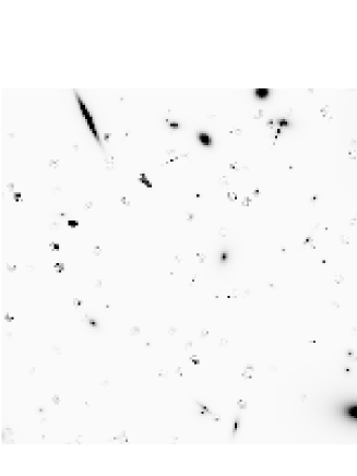
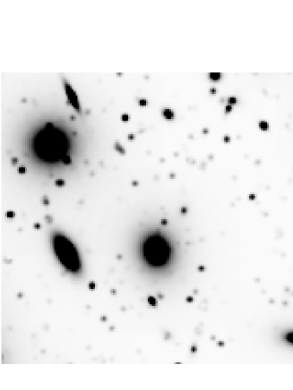
(a) Field galaxies                                     (d) Convolved with Gaussian

                                                            

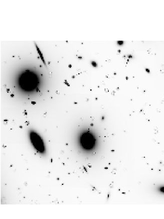
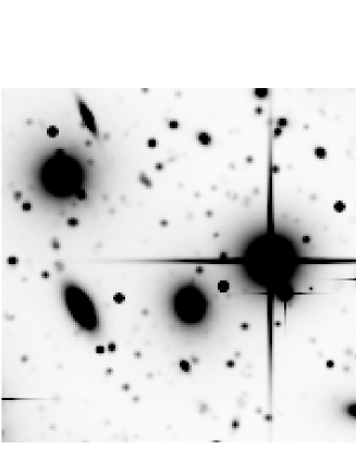
(b) Cluster added                                     (e) Stars added

                                                            

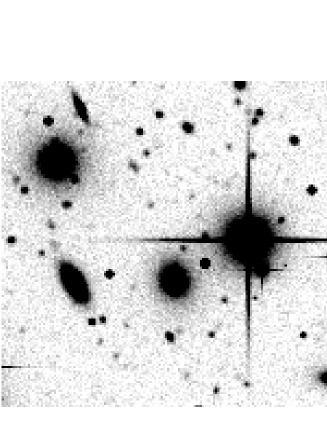
(c) Shot Noise added                                (f) Sky noise added

Figure 1: An illustration of the process of simulating a section of a sight-line through a cluster. The simulated field of view is 1 sq arcmin, pixels size is 0.39 by 0.39 arcsecs and the seeing FWHM is 0.9^′′.

Figure 1 shows a montage of six images, illustrating the development of a simulated image through the stages previously outlined. The panels from top to bottom and left to right show a 1 by 1 arcmin section of a simulated cluster image at various stages: (a) simulated field galaxies, all types; (b) cluster galaxies added; (c) with shot noise added (barely noticeable at the grey levels chosen); (d) after convolution with a 0.9^′′ FWHM Gaussian “seeing” disk; (e) with stars added; and finally, (f) with sky noise added. Note in particular the fattening and shortening of edge–on disks, the loss of faint objects and the loss of low surface brightness objects as these various processes are applied.

3 Detection Software

Our chosen object detection and photometry package is SExtractor described in detail by Bertin & Arnout (1996). The finding algorithm used by SExtractor searches for galaxies with a minimum number of connected pixels above a specified background after convolution with a preset filter; in this case a $3\times 3$ top-hat filter. Each detection is then re-analysed and a number of detailed measurements made, including: corrected isophotal magnitude, Kron magnitude, isophotal area and a star/galaxy estimation. Note that the SExtractor package adopts Kron magnitudes when the object is isolated and uses the corrected isophotal magnitude for crowded regions. In addition SExtractor has a logical strategy for dividing blended objects into components based on the ratio between the sub-peaks and the total flux.

Kron magnitudes are used for estimating total fluxes and are based on the Kron radius which is defined as: $R_{K}=\frac{\sum I(r)r\delta r}{\sum I(r)\delta r}$ (Kron 1978). The magnitude is normally measured through an aperture of radius $r=2.5R_{K}$, which is that recommended for the inclusion of $>90$% of the flux for ellipticals and spirals. To test how the irregulars faired we measured the flux for random samples of 54 galaxies of each type with constant magnitude of $m_{R}=18.0$ and varied the aperture radius from 2.0–5.0 $R_{K}$. Table 2 shows the resulting flux returned based on the following specific types: Ellipticals with $M_{R}=-22.0$ mags, ($\mu_{o}=-13.0$ mags per sq arcsec); mid-type spirals with $M_{R}=-20.0$ mags, ($\mu_{o}=-19.3$ mags per sq arcsec); irregulars with $M_{R}=-17$ mags, ($\mu_{o}=-21.7$ mags per sq arcsec); and dwarf ellipticals with $M_{R}=-18.0$ mags, ($\mu_{o}=-19.0$ mags per sq arcsec). On the basis of these tests a more conservative radius of $r=3.5R_{K}$ was selected such that our photometric error is less than the typical magnitude zero point error expected in our data ($\Delta m=\pm 0.05$). As a further test of both the galaxy simulations and the SExtractor software we simulated $\sim 4000$ galaxies of each type ranging from $m_{R}=18$ to $m_{R}=26$ and added noise equivalent to $m_{R}=26.0$ mags arcsec^-2.

Figure 2 shows the resulting median magnitude difference (errorbars are the upper and lower quartiles) versus the known simulated magnitude, for the five object types. Also shown in Figure 2 are the theoretical upper and lower quartiles for a perfect point source (star) convolved with the simulated Gaussian sky noise fluctuations. From Figure 2 we can see that the fluxes are both accurately allocated and measured, regardless of galaxy type and orientation over bright magnitudes. The discrepancy for the brightest stars is due to the simulated diffraction spikes which extend outside of the $r=3.5R_{K}$ aperture and are present for $m_{R}<18.5$ only. For all galaxy types magnitudes become unreliable ($\Delta m>$ 0.1) at $m_{R}\approx 24$ and totally unreliable fainter than $m_{R}\approx 24.5$; note that this is 1.5 mags above the theoretical $1\sigma$ point source detection limit! Figure 3 shows the corresponding fractional completeness as a function of input magnitude. It can be seen that incompleteness becomes significant at $m_{R}\approx 24.0$; the completeness drops to 90% completeness at $m_{R}=23.95$, $m_{R}=24.3$, $m_{R}=24.0$ and $m_{R}=24.4$ for ellipticals, mid-type spirals, irregulars and dwarf ellipticals, respectively. Stars fall below the 90% completeness limit beyond $m_{R}=24.25$. That the ellipticals are ’lost’ first is a testimony to the power of cosmological surface brightness-dimming or the “cosmic guillotine” effect (see Koo & Kron 1993).

4 Cluster Simulation

4.1 Cluster type

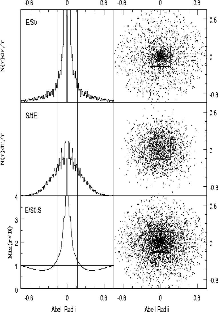
Figure 4: The density profiles for ellipticals (upper left), for spirals and for dwarf ellipticals (middle left) and the morphological mix of E/S0:Spirals as a function of Abell radius (lower left), the square box within the panels represents the equivalent field of view for the observational data presented in Paper III. The right panel shows the projected density of elipticals (upper right), spirals (middle right) and ellipticals and spirals (lower right).

There are typically three major classifications of cluster type as listed in Oemler (1974): spiral-rich, cD-dominated or spiral-poor. These three different types of cluster are associated with an irregular or flat profile, fully viralised radial profile (1/$r$) or a semi-relaxed intermediary profile, respectively. A strong relation between morphology and local projected galaxy density is also seen across all 3 cluster types with a smooth transition between an E/S0-dominated mix in the higher density regions to one which is spiral-dominated in the lower density regions (Dressler 1980). In the regular cD and spiral-poor clusters, this results in an elliptical distribution which is much more centrally concentrated than that for spirals. To accommodate this, we adopt two principle profile shapes. These two profiles are: a purely radial 1/$r$ distribution giving a centrally concentrated population (consistent with the distribution of ellipticals), and, a Gaussian distribution where the FWHM is 1 Mpc or 1/3 of the Abell radius (consistent with the less concentrated spiral distribution). Hence to simulate a cD or spiral poor cluster we require a cluster with a high density of ellipticals distributed in a (1/$r$) profile and a low density of spirals distributed in a Gaussian. The net result for the overall profile is a slightly extended (1/$r$) profile consistent with the formulation of a cD cluster as presented in Oemler (1974). Similarly for a spiral-rich cluster we have an equal density of ellipticals and spirals resulting in an overall profile with a predominantly Gaussian distribution again consistent with the specification of Oemler (1974) i.e. by changing the morphological mix we are also changing the cluster profile shape. Figure 4 shows the two profiles (left side; elliptical (1/$r$) profile (upper) and spiral Gaussian profile (middle)) and the equivalent projected density distributions (right side). A practical modification is made to the (1/$r$) profile by randomising positions within the central 100 kpc as a purely (1/$r$) profile produces an unrealistic number of galaxies at the cluster centre.

4.2 The Reference Cluster

For the simulations presented in this and the next section, it was convenient to define a reference cluster. The strategy is that once the reference cluster has been defined we can then explore deviations from this parameter space rather than simulate all possible clusters (which for obvious reasons is impractical). We model our reference cluster on the parameter space for which we have obtained most of our data, i.e. spiral-poor richness 3 clusters at redshift $\sim 0.15$. Hence we adopt the cluster profiles for ellipticals and spirals as discussed above with a morphological mix ratio of E/S0:Sabc of 1:1. The lower panels in Figure 4 show the morphological mix as defined within some fraction of the Abell radius (left) and the combined projected density distribution of ellipticals and spirals (right). For the dwarf ellipticals, we found in Paper I that the lower luminosity population is much less strongly clustered (even after consideration of the difficulty of detecting dwarfs in the cluster core); we therefore also select a Gaussian profile distribution for this population.

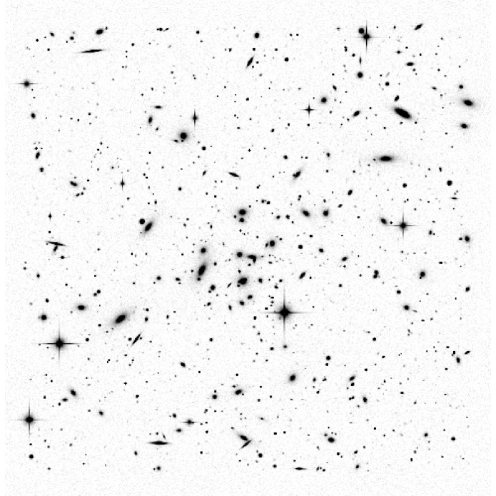
Figure 5: An example simulated sight-line through our reference cluster.

Figure 5 shows an example simulation of our reference cluster and the strong central clustering of ellipticals is clearly apparent. A comparison field region has also been simulated (although not shown) and the number counts for both images determined using the SExtractor software as described earlier. The final counts are corrected for the diminishing area available to fainter objects (see Paper I for details). Figure 6 shows the resulting number-counts and here we compare the input and detected number-counts for (a) the field, and (b) the cluster + a second independent field. The lower panel of Figure 6 shows the recovered LD for this cluster compared to the known input LD. Note that in this single simulation, $\sim 1200$ galaxies are detected in the field image and $\sim 1500$ galaxies are detected in the cluster image (i.e. $\sim 2700$ total galaxies detected out of $\sim 5100$ simulated for the two sight-lines). The completeness limit ($m_{R}\approx 24$), as defined by the departure of the detected number-counts from the known input number-counts, is in agreement with the earlier photometric tests. The recovered LD for our reference cluster is a good representation of the input distribution demonstrating the qualitative validity of the technique. In order to evaluate the match quantitatively we apply a Kolmogorov-Smirnov Two-Sample Test. A two sample test is applied as the input distribution is itself drawn from the initially specified smooth LFs (as we are sampling only a portion of the cluster’s population). The KS value is determined in the normal manner, i.e. both distributions are normalised to unity within the magnitude range of comparison and the cumulative distributions compared, the largest discrepancy between the two distributions is then the KS value. To evaluate the probability of these two distributions being the same we convert the KS value to a $\chi^{2}$ value and determine the probability from the incomplete gamma function. The conversion is given by Wall (1996):

$$\chi^{2}=4(KS)^{2}\frac{N_{i}N_{o}}{N_{i}+N_{o}},$$ (2)

where $N_{i}$ is the input number of cluster galaxies above our magnitude cutoff and $N_{o}$ is the observed number of cluster galaxies above our magnitude cutoff.

We now define a ‘goodness-of-fit’ parameter, GOF, to be the evaluated $\chi^{2}$ probability of the two distributions being the same, expressed as a percentage. Hence for the single simulation shown in Figure 6 the GOF=94.7 %. Since a single simulation may be unrepresentative due to a statistical vagary in this particular arrangement of stars and galaxies, we repeat the measurement a number of times and estimate the mean GOF and its standard deviation. Figure 7 shows the recovered LDs compared to the actual LDs and the individual GOFs for eleven simulations of our reference cluster. In all cases the agreement is good to excellent. (Note that a total of 22 sight-lines or $\sim 56,000$ galaxies were simulated). The lower right panel of Figure 7 shows the average LDs; the mean overall GOF of the eleven simulations is 93 $\pm 4$ %.

5 The Simulations

We now explore the validity of our technique for recovering a cluster’s LD over a wider range of parameter space. To determine the optimal parameter values we adopt a reference cluster ($z=0.15$, Richness = 3, $\alpha=-1.0$, E:S0/Sabc mix = 1:1) and investigate deviations from this scenario by adjusting one parameter at a time. In particular we wish to determine how far our technique for LD recovery can be applied in terms of cluster redshift and cluster richness and to assess its dependence on observables such as seeing conditions and zero magnitude point errors. In each case we simulate eleven realisations of each scenario over the range of parameters we wish to explore.

These simulations require the specification of detector parameters such as field-of-view (f.o.v.), pixel size, noise, exposure time etc. Here we model our simulations on the observational configuration used in collecting our new data (Paper III): the f/3.3 prime-focus of the 3.9 m Anglo-Australian Telescope (AAT) equipped with a Tektronix 1K² CCD, giving 0.39 arcsec pixels, a field-of-view of $6.5\times 6.5$ arcmin and an exposure time of 90 mins.

5.1 The morphological mix

We have already discussed the three principle cluster types which are distinguished by the variation from dense, cD-dominated, spiral-deficient to the more loosely bound spiral-rich clusters. Hence it is clear that we must consider the morphological mix and profile shape together. The definition of our cluster profile is such that an entirely spiral-deficient cluster will have a (1/$r$) profile and a spiral-rich cluster a Gaussian profile. Hence by simply adjusting the morphological mix ratio of ellipticals to spirals we explore, simultaneously, both the morphology and profile dependence of the technique. Figure 8a shows the GOF results, with each point calculated from the mean of 11 simulated clusters and field sight-lines. The simulations span the E/S0:Sabc mix range in steps from 4:1 to 1:1 (where the mix is defined within the Abell radius). The errorbars indicate the standard deviation of the values (not of the mean i.e. we have not divided the errors by $\sqrt{N}$), so that they more reflect the range of GOFs from individual values rather than the accuracy to which we have evaluated the mean GOF. The flat GOF shows that the technique is insensitive (at these redshifts, richnesses etc) to the morphological mix and profile shape. The former is hardly surprisingly as at the faint limits morphological information is lost while at brighter limits we do not expect any bias nor have we detected any in our photometric tests. The latter is perhaps more surprising as one might expect the denser profile to be more confused; nevertheless the results indicate this is not a significant concern.

5.2 The faint end slope

As stated previously, much attention has recently been drawn to the faint end slope of the luminosity function, the clusters observed so far all exhibiting an apparently universal dwarf-rich LD (Paper I). The question of whether the same form might also be true of the field LF is highly topical (Phillipps & Driver 1995; Driver & Phillipps 1996). However, we first need to ask whether the technique can reliably recover any shape of LD. To explore this possibility we adopt the reference cluster and vary only the faint slope parameter for the dwarf ellipticals, i.e. the $\alpha$ parameter in the adopted dE Schechter function (Schechter 1976). In this simulation we explored the range $-0.5<\alpha<-2$ with $M_{R}^{*}=-19.0$ and $\phi_{dE}^{*}=\phi_{E}^{*}$. The results are shown in Figure 8b and indicate that our technique yields an acceptably high GOF for any faint end slope. The lowest GOF value of $85\%$ occurs for a steeply declining faint end LF slope. Results are marginally more reliable for the previously observed values of $\alpha\sim-1.5$. These simulations therefore add significant weight to the results of Paper I.

5.3 Cluster richness

The Abell richness parameter varies within the ACO catalogue (Abell, Corwin & Olowin 1989) from a value of 0 to 5. Richness is defined as 0, 1, 2, 3, 4 or 5 if the number of galaxies in the range $m_{3}$ to $m_{3}+2$ within the Abell radius is: 30—49, 50—79, 80—129, 130—199, 200—299, 300 or over, respectively, where $m_{3}$ is the magnitude of the third brightest object in the cluster. The main concern with the LD recovery technique is that it relies on the contrast of cluster members being significant in comparison to the typical field-to-field variation from one sight-line to the next. To examine this we simulated clusters over the whole range of richness by adjusting the $\phi_{*}$ values of the three cluster LFs. To reduce the coarseness of the richness class scale we also devised half richness classes. Figure 8c shows the results and clearly cluster richness is of paramount importance. The drop in GOF occurs rapidly for richnesses less than 1.5 suggesting there is little reliability in the reconstruction of the LDs of poor clusters. Going to a large format CCD, giving a larger f.o.v. is likely to partially alleviate the problems. In these simulations we have reduced the dwarf component in line with the luminous galaxies to preserve an overall flat LF. If the density of dwarfs is independent of giants we may have biased our results adversely. The net result is that a richness limit of 1.5 is a realistic lower-limit if the cluster LF is indeed flat in these environments, but which may need to be re-evaluated if the dwarf and giant densities are unrelated.

5.4 Cluster redshift

If a cluster is too near then the physical extent seen by a contemporary CCD will be small and consequently fewer cluster members will be seen. Conversely, at large distances, the cluster may become confusion limited, unresolved (i.e. cluster diameter smaller than f.o.v.) or simply too faint for our technique to work. Figure 8d shows the results from a set of simulations spanning the redshift range 0.0 to 0.5. The results indicate that both of these concerns are valid. For the simulated f.o.v. chosen (6.5 by 6.5 arcmins²) the optimal redshift for this technique appears to lie in the range $0.1<z<0.3$. At a completeness limit of $m_{R}=24.0$ this equates to an absolute magnitude limit in the range $-15<M_{R}<-17$ respectively. Wider f.o.v. detectors (mosaics or photographic emulsions) are likely to be more appropriate for examining low redshift clusters although stellar and background confusion (Drinkwater et al. 1996) are more severe. At the high redshift end it is clear that compactness of the cluster core leads to a severe confusion limit. However, it is likely that Hubble Space Telescope WFPC2 observations will extend the reliability of the technique to higher redshifts.

5.5 Seeing

We test the effect of the seeing in order to assess when the observing conditions become too poor for our technique. Again we adopt the reference cluster and Figure 8e shows the results of varying the seeing FWHM. As expected the GOF deteriorates badly in seeing worse than 2^′′ where the fainter galaxies are simply blended in with the bright ones or the mean surface brightness of compact objects falls below the detection threshold. The technique does seem to be almost independent of seeing over the range 0^′′ to 1.5^′′. Surprisingly there is a slight tendency for $\sim 1^{\prime\prime}$ seeing to give a better result than sub-arcsec seeing. This is likely to be due to two factors: The simulated pixel size and the over de-blending of irregulars by the SExtractor software. In these simulations, 0.39^′′ pixels have been used and in sub-arcsecond seeing, compact objects and noise spikes become indistinguishable, raising the level of confusion. The second problem of de-blending is due to the complex structure of the simulated irregulars which in $\sim 1^{\prime\prime}$ seeing are unresolved but in sub-arcsec seeing may be de-blended into several objects (c.f. Figure 1a). It would appear, therefore, that seeing of FWHM $\sim 1^{\prime\prime}$ is optimal for providing the best GOF results. Pixel size is also likely to be important, although we have not explored this here. It is possible that the decline of the GOF in good seeing is related to undersampling of the seeing disk. Of particular curiosity is the dramatic dip in the GOF at a FWHM of 2.1^′′; the variation in the eleven simulations indicate that this is not a random error but is somehow systematic.

5.6 Zero point error

An alternative explanation to the turn-up seen in A963 (Driver et al. 1994a) is that there was a photometric zero point error between the cluster and field sight-lines. There is some justification for this concern, as the instrument with which the data were obtained, “Hitchhiker”, was a parallel instrument for which calibration data were collected sporadically and instrument consistency was relied upon. This criticism has been partly mitigated by recent observations of other rich clusters with well calibrated data which have revealed similar LDs to A963 (c.f. Wilson et al. 1997). Nevertheless it seems prudent to ask how accurate the photometry must be for the technique to be valid. Here we adjust the photometric zero magnitude point of firstly the cluster sight-line and then the field sight-line. The resulting GOF curve is not shown but the mean GOF was found to fall below 80% if the photometric zero points are in error by greater than $\Delta m=\pm 0.12$. (For a field number count slope around 0.4 this implies a relative error of 12% in numbers between sight lines).

6 Conclusions

The simulations presented here demonstrate the validity of applying a purely statistical photometric method to reconstruct a cluster’s Luminosity Distribution (LD). The simulations are used to generate detailed CCD images of field and cluster sight-lines and incorporate factors such as: morphological types (E, Sb, Irr, dE & Stars); morphological field luminosity functions; surface-brightness luminosity dependencies; cosmological effects (surface brightness dimming, K-corrections, luminosity and angular distances); ellipticities, inclinations and disk axis-ratios; object overlap; cluster profiles (1/r, Gaussian), richness, redshift, luminosity function, morphological mix and crowding; noise processes (shot-, sky-, unresolved objects); stellar contamination; atmospheric seeing; detector and instrumental characteristics; image detection and photometry. Not simulated are: cosmic rays; CCD read-out noise, dark current and defects; and opacity (our simulations assume all objects are optically thin). Several thousand sight-lines were generated each containing several thousand objects with morphological number-counts matched to deep Hubble Space Telescope observations, images were created and galaxy catalogs generated in an identical manner to the data presented in Paper III. The derived cluster LDs were compared to the input distributions via a Kolmogorov-Smirnov statistical test to assess accuracy. As an aside we note that an accurate and complete faint galaxy catalogue can only be generated to a magnitude limit well above the point source detection limit. For a fully sampled seeing disk of $1^{\prime\prime}$ this limit is 2 magnitudes (i.e. for a point source detection limit of 26 mags the catalogue would only be complete and reliable to a limit of 24 mags).

As the accuracy of the method is dependent on both the cluster properties and the detector characteristics it is not possible to define universally the cluster space over which the method is valid. Instead we demonstrate the specific cluster parameter space for our chosen detector through which the data presented in Paper III were collected. Hence the simulations presented here were specifically to mimic a 90 minute exposure on the Anglo-Australian Telescope’s f/3.3 Tek 1K² 24$\mu m$ pixel CCD (pixel size 0.39 by 0.39 arcsecs, f.o.v. 6.5 by 6.5 arcmins), but should be applicable to any similar field-of-view detector. The primary results for this setup are summarised as follows:

(i) the cluster richness must be greater than 1.5,

(ii) the cluster should lie in the redshift range $0.1<z<0.3$,

(iii) the FWHM of the seeing must be less than 1.25^′′.

(iv) the technique is independent of cluster type (i.e. morphological mix or profile shape) for the shapes and mixes explored.

(v) the technique can recover the faint end slope of the cluster LD for any shape distribution

(vi) photometric zero points must be accurate to $\Delta m=\pm 0.12$.

The simulations have demonstrated that for a given detector and exposure time there is a range of observable parameter space over which the cluster LD reconstruction method is valid and beyond which results are questionable. Detailed and exhaustive simulations such as those presented here are therefore vital and essential to establish the credibility of this technique for any specified dataset. Within the valid boundaries the technique is extremely time efficient, simple and likely to make a substantial contribution to the study of cluster populations over a range of redshift and environment. Finally we note that the simulation software can generate data for any detection setup, field-size etc for cluster or field images. Other groups wishing to use this software are encouraged and should contact spd@edwin.phys.unsw.edu.au

References

Abell G.O., 1958, ApJ. Supp., 3, 211

Abell G.O., Corwin Jr H.G., Olowin R.P., 1989, ApJ. Supp., 70, 1

Bernstein G.M., Nichol R.C., Tyson J.A., Ulmer M.P., Wittman D., 1995, AJ, 110, 1507

Bertin E., Arnout, S., 1996, Astr. Astrophys. Suppl., 117, 393

Binggeli B., 1994, in ESO/OHP Workshop proceedings on Dwarf Galaxies, eds G. Meylan and P. Prugniel (ESO)

Biviano A., Durret F., Gerbal D., Le Fevre O., Lobo C., Mazure A., Slezak E., 1995, A & A, 297, 610

Boroson T., 1981, Ap J Supp, 46, 177

Broadhurst T., 1998, ApJL, submitted (astro/ph9511150)

Coleman, G.D., Wu, C.C., Weedman, D.N., 1980, Ap J Supp, 43, 393

de Propris R., Pritchet C.J., Harris W.E., McClure R.D., 1995, ApJ, 450, 534

de Vaucouleurs G., 1959, Handbuch der Physik, 53, 311

Disney M.J., 1995, in “Opacity of Spiral Galaxies”, eds Davies J.I., and Burstein, D., (Dordrecht, Kluwer), p 5

Dressler, A., 1980, Ap J, 236, 351

Driver, S.P., Couch W.J., Phillipps S., 1998, MNRAS, in press (Paper III)

Driver, S. P., Phillipps, S., Davies, J. I., Morgan, I., Disney, M.J., 1994a, MNRAS, 268, 393

Driver, S. P., Phillipps, S., Davies, J. I., Morgan, I., Disney, M.J., 1994b, MNRAS, 266, 155

Driver, S. P., Windhorst, R. A., Griffiths R. E. 1995, ApJ, 453, 48

Driver, S.P., Windhorst, R. A., Ostrander, E.J., Keel W.C., Griffiths, R. E., Ratnatunga, K.U., 1995, ApJL, 449, L23

Driver, S.P., Phillipps, S., 1996, ApJ, 469, 529

Drinkwater, M.J., Currie M.J., Young C.K., Hardy E., Yearsley J.M., 1996, MNRAS, 279, 595

Ferguson, H.C., Binggeli., 1994, A&ARv, 6, 67

Freeman K.C., 1970, ApJ, 160, 811

Glazebrook, K., Ellis, R. S., Colless, M. M., Broadhurst, T. J., Allington-Smith, J., Tanvir, N., 1995, MNRAS, 273, 157

Glazebrook, K., Ellis, R. S., Santiago, B., Griffiths, R.E., 1995, MNRAS, 275, 19pp

Holmberg E., 1946, Medd. Lunds Obs II, No 117

Hubble E., 1926, ApJ, 64, 321

Impey C.D., Bothun G.D., Malin D.F., 1988, Ap J, 330, 634

King C.J., Ellis, R.S., 1985, ApJ, 288, 456

Kron R.G., 1978, PhD Thesis, University of California at Berkeley

Marzke, R.O., Geller, M.J., Huchra, J.P., Corwin Jr, H.G., 1994, A J, 108, 437

Metcalfe, N., Shanks, T., Fong, R., Roche, N., 1995, MNRAS, 273, 257

Odewahn S.C., Windhorst R.A., Driver S.P., Keel W.C., 1996, ApJ, 472, L13

Oemler Jr, A., 1974, Ap J, 194, 1

Pence W., 1976, Ap J, 203, 39

Phillipps, S., Davies, J.I., Disney, M.J., 1990, MNRAS, 242, 235

Phillipps, S., Driver, S.P., 1995, MNRAS, 274, 832

Sandage, A., 1961, Ap J, 133, 355

Schechter, P., 1976, Ap J, 203, 297

Simien, F., de Vaucouleurs, G., 1986, Ap J, 302, 564

Smith, R.M., Driver, S.P., Phillipps, S., 1997, MNRAS, 287, 415 (Paper I)

Trentham N., 1997a, MNRAS, 286, 133

Trentham N., 1997b, MNRAS, 290, 334

Trentham N., 1998, MNRAS, 295, 360

Wall J.V., Quarterly Journal of the R.A.S., 1996, 37, 519

Williams R.E., et al. 1996, AJ, 112, 1335

Wilson, G, Smail, I., Ellis, R.S., Couch, W.J., 1997, MNRAS, 284, 915

Appendix A Simulation details

The description in §2 defines the generic galaxy types which we shall consider. Specific details (i.e. actual numbers) have been listed in Table 1. The most important a priori decision was the opacity. While detailed models are available to cope with opacity, here we decide to assume all objects are optically thin at all radii (i.e. zero opacity). The main motivation for this, apart from the fact that the true opacity of disk systems is not known (c.f. Disney 1995), is that the majority of objects simulated will be barely resolved and the additional computational time required to compute the effect of opacity was not justified. Setting opacity to zero also simplifies the simulation process as the apparent magnitude of an object remains fixed regardless of inclination. This in turn, allows us to fully define a galaxies light-profile simply from its absolute magnitude ($M$), intrinsic surface brightness ($\mu_{o}$), and apparent magnitude ($m$) (plus a randomly selected orientation/ellipticity).

A.1 Cosmological Model

Our software, which generates the simulated profiles, uses the output from our number-count software (c.f. Driver, Windhorst & Griffiths 1995) which (taking a normalisation parameter for each LF type) generates a list of number-counts, N(M,m,T). The specification of type (T) and absolute magnitude also defines the intrinsic face-on surface brightness ($\mu_{o}$, or in intensity units $I_{o}$), if we assume the relationships of Table 1 (taken from Binggeli 1994). By assuming zero opacity, the redshift ($z$) can be derived via the relevant distance-luminosity relation only (i.e. without requiring knowledge of inclination etc). Here the cosmological model we have chosen is the standard model of a flat expanding universe, with $H_{0}$ = 50 km s^-1 Mpc^-1, $\Omega$ = 1, $\Lambda$ = 0, $q_{0}$ = 0.5. The effects of such a model on the visibility of galaxies is discussed in Phillipps, Davies & Disney (1990) and the distance luminosity relation is defined as:

$$M=m-5\log{d_{l}}-25-k_{c}(z),$$ (3)

where $d_{l}$, the luminosity distance, is dependent on the World model:

$$d_{l}=(1+z)2cHo^{-1}[1-(1+z)^{-1/2}],$$ (4)

and $k_{c}(z)$ is the K-correction.

Evaluating the above gives $z$ and within this cosmological model the apparent ($I_{o}^{app}$) and intrinsic ($I_{o}$) face-on central surface intensities are related by:

$$I^{app}_{o}=\frac{I_{o}10^{-0.4k_{c}(z)}}{(1+z)^{4}}.$$ (5)

This gives us the apparent face-on central surface brightness of the object which, with the known apparent magnitude (m) and type, fully defines the light profile.

A.2 Light Profiles

The basic light-profile for all galaxy types is assumed to follow the generalized form:

$$I(r)=I_{o}exp\left(-\left(\frac{r}{a_{o}}\right)^{\frac{1}{\beta}}\right)$$ (6)

where, $I(r)$ is the intensity at a radius $r$, $a_{o}$ is the face-on scale-length, $\beta=1$ for pure disks, (Freeman 1970) and $\beta=4$ for ellipticals (de Vaucouleurs 1959).

Integrating this light profile over a galaxy’s total face-on area gives the total luminosity:

$$L_{Total}=(2\beta)!\pi I_{o}a_{o}^{2}$$ (7)

or in magnitude units;

$$m=\mu^{app}_{o}+5\log(a_{o})+2.5log((2\beta)!\pi)$$ (8)

Hence as m, $\mu^{app}_{o}$ and $\beta$ are already known, $a_{o}$ is defined.

The final stage is the randomisation of orientation. For ellipticals we simply allocate an ellipticity assuming equal probability for all ellipticities from E0 to E7 and define the product of the major and minor axis to equal $a_{o}$, the E0 scale-length. For other types we allocate an inclination angle $\theta$ in the range 0—90 degrees and compute the ellipticity as described by Eqn 1, (c.f §2.1). Hence the surface brightness of ellipticals is constant regardless of ellipticity, however the central surface brightness of disks is dependent on inclination as: $\mu^{app}_{o}=\mu^{app}_{i}-2.5\log(cos\theta)$ Boroson (1981). Finally the elliptical light-profile is simulated by randomly selecting a position angle and converting the circular intensity light-profile (Eqn 6) to that for an ellipse:

$$I(r,PA)=I^{app}_{i}\exp\left(-\left(\frac{r\sqrt{a^{2}cos^{2}(PA)+b^{2}sin^{2}(PA)}}{a^{app}_{i}}\right)^{\frac{1}{\beta}}\right)$$ (9)

where a and b are the major and minor axis with their product equal to unity.

Tables

Table 1: The intrinsic parameters and assumptions used for the simulations for each of the four generic galaxy types.

Property	elliptical	mid-type spiral	irregular	dEs
$M^{*}_{R}$	$-22.3$	$-21.7$	$-21.2$	N/A
$\alpha$	$-0.9$	$-0.8$	$-1.8$	N/A
$\phi_{*}$	$1.14\times 10^{-3}$	$1.74\times 10^{-3}$	$2.50\times 10^{-4}$	N/A
Profile	$I_{r}=I_{o}exp(-\frac{r}{a}^{\frac{1}{4}})$	$I_{r^{Bulge}}=I_{o}exp(-\frac{r}{a}^{\frac{1}{4}})$	$I_{r}^{Global}=I_{o}exp(-\frac{r}{a})$	$I_{r}=I_{o}exp(-\frac{r}{a})$
		$I_{r}^{Disk}=I_{o}exp(-\frac{r}{a})$	$I_{r}^{Local}=0.05I_{o}exp(-\frac{r}{a})$
$\mu_{o}$	$\mu_{R}$=$17.6-(M_{R}+26.4)$	$\mu_{R}$=19.3	$\mu_{R}$=19.8+0.8($M_{R}$+18.9)	$\mu_{R}$=16.6+($M_{R}$+20.4)
$(B-R)$	1.8	1.4	0.9	1.8
Ellipticity	0.0—0.7	0.0—0.8	0.0—0.5	0.0—0.3
KR-corr	$1.36z+1.07z^{2}$	$0.40z+0.71z^{2}$	$0.05z+0.78z^{2}$	$1.36z+1.07z^{2}$

The parameters for this table are taken from the following sources: $M_{R}^{*}$ & $\alpha$, Marzke et al. (1995); $\phi_{*}$, Driver et al. (1995); $Profiles$, Freeman (1970) for disks and de Vaucouleurs (1959) for ellipticals; $\mu_{o}$, Binggeli (1994); $(B-R)$, Coleman, Wu & Weedman (1980); $Ellipticity$, Sandage (1961) and Hubble (1926); $K-corrections$, Driver et al. (1994b, and originally from Pence 1976 and King & Ellis 1985).

Table 2: The measured flux for the four types of simulated galaxy as a function of aperture size (defined in terms of Kron Radii). All galaxies were simulated to have $m_{R}=18.0$ and the tabulated values are the median measured value for 54 randomly simulated examples for each type.

Aperture Radius	E	Sb	Irr	dE
2.0$R_{K}$	18.16	18.05	18.01	18.02
2.5$R_{K}$	18.16	18.05	18.01	18.02
3.0$R_{K}$	18.14	18.04	18.00	18.01
3.5$R_{K}$	18.11	18.02	18.00	18.01
4.0$R_{K}$	18.09	18.02	18.00	18.00
4.5$R_{K}$	18.07	18.01	18.00	18.00
5.0$R_{K}$	18.06	18.01	18.00	18.00

                                                            

Figure 2: The difference between the measured magnitude and allocated magnitude for the four types of simulated galaxies and simulated stars. The solid line indicates the zero discrepancy line. The thick lines indicate the theoretical upper and lower quartiles based on the adopted sky noise. 54 isolated objects at random orientations were simulated from $m_{R}=18.0$ to $m_{R}=26$ at 0.1 magnitude intervals.

Figure 3: The fractional completeness for the simulations shown in Figure 2, as a function of input magnitude.

Figure 6: The number-count plots for the comparison field (upper left), cluster sight-line (upper right) and the excess as compared to the known input distributions (lower panel). The solid straight lines show the mean galaxy counts from Metcalfe et al. (1996) for reference.

Figure 7: The recovered LDs compared to input LDs for 11 realisations of our reference cluster. The bottom right panel shows the average results.

Figure 8: Simulation results investigating the method’s dependence on: (a) morphological mix, (b) faint end slope, (c) richness, (d) redshift and (e) seeing.