Galactic H emission and the Cosmic Microwave Background
Abstract
We present observations of Galactic emission along two declination bands where the South Pole cosmic microwave background experiment reports temperature fluctuations. The high spectral resolution of our Fabry–Perot system allows us to separate the Galactic signal from the much larger local sources of emission, such as the Earth’s geocorona. For the two bands (at °and °), we find a total mean emission of R with variations of R. The variations are within the estimated uncertainty of our total intensity determinations. For an ionized gas at K, this corresponds to a maximum free–free brightness temperature of less than 10 K at 30 GHz (K–band). Thus, unless there is a hot gas component with K, our results imply that there is essentially no free–free contamination of the SP91 (Schuster et al. 1993) and SP94 (Gunderson et al. 1995) data sets.
Key Words.:
Cosmology: –cosmic microwave background, –diffuse radiation, Galaxy: –halo, ISM: lines and bands1 Introduction
Cosmology has entered the era of precision cosmic microwave background (CMB) measurements. Since the original detection of temperature perturbations on large angular scales by the COBE satellite (Smoot et al. 1992), there has been a myriad of new detections, resulting in a data set spanning roughly two orders of magnitude in angular scale (Lineweaver et al. 1997; White et al. 1994). The extraction of cosmological information requires careful control and understanding of all possible sources of signal contamination. The current quest for high precision determination of cosmological parameters (Jungman et al. 1996; Knox 1995) demands a correspondingly greater understanding of all foregrounds. In particular, the Galaxy, via synchrotron, dust and free–free emission (Bremsstrahlung), represents a source of foreground brightness fluctuations which all experiments must recon with. These three contaminating emissions define a “valley” in the brightness–frequency plane centered around 90 GHz, representing the point of smallest Galactic contamination (Kogut et al. 1996a). Although, clearly, CMB efforts are concentrated in this “valley”, Galactic signals must nonetheless be carefully removed to extract the purely cosmological fluctuations and to achieve the desired precision on cosmological parameters.
The removal of these foregrounds is usually done in one of two ways. With sufficient frequency coverage and a high signal–to–noise ratio, a spectral analysis of the CMB data alone can in principle distinguish the Galactic foregrounds from the CMB signal. The other approach is to use sky maps made at other frequencies as templates and to extrapolate a given foreground emission into the CMB bands according to its spectral dependence. Even when the quality of the CMB data permits the former technique, the second approach provides an important, external check on the removal procedure. For synchrotron emission, one usually uses the 408 MHz Haslam map (Haslam et al. 1981) and the 1420 MHz survey (Reich & Reich 1986) as a template (uncertain spatial variations of the synchrotron frequency index renders the procedure slightly less straightforward than one would hope). The IRAS all sky survey serves as a useful template for dust emission on angular scales under °, and it is usually augmented with DIRBE maps on larger angular scales (as with synchrotron emission, uncertainty in the exact slope of the dust emission law introduces an unfortunate complication).
In this paper, we address the question of Galactic free–free emission in relation to CMB anisotropy measurements (two recent reviews are given by Smoot 1998 and Bartlett & Amram 1998). Among the three Galactic sources of troublesome microwave emission, free–free emission is the most difficult to control. This is because the only frequency range in which it dominates over dust and synchrotron emission is in the CMB valley; in other words, one cannot extrapolate maps made at much lower or higher frequencies into the CMB valley to remove free–free contamination. What is needed is a tracer of the warm ionized interstellar medium (WIM) responsible for free–free emission. Given that at high Galactic latitudes there is minimal extinction from dust, one expects Hydrogen line emission in the excited gas to be a good possibility for such a tracer.
The line emission is measured in Rayleighs (1R photons cm-2 s-1 ster-1 erg cm-2 s-1 ster-1 at Å) and may be expressed in terms of the temperature and emission measure, , of the WIM for Case B recombination:
| (1) |
where K; this expression is valid for temperatures (e.g. Reynolds 1990), more accurate formulae are given by Valls–Gabaud (1998). Free–free emission depends on the same quantities (given here for pure Hydrogen and in the limit as ):
| (2) |
where is the brightness temperature, the observation frequency is Hz, and is the thermally averaged gaunt factor, which to 20% for few is
| (3) |
(e.g. Smoot 1998). Thus, the free–free brightness associated with a given intensity is approximately
| (4) |
Valls-Gabaud (1998) discusses more accurate expressions. There does not, as of yet, exist a complete survey of the sky in , and the distribution of the warm ionized medium (WIM) of our galaxy remains somewhat of a mystery. Local sources pose the most serious difficulties for efforts to measure the Galactic emission. The Earth’s geocorona emits in with an intensity of R, depending on the season, the solar activity and the solar depression angle. This is an order of magnitude larger than the typical signal we expect at high Galactic latitude. In addition, there is an OH line from the atmosphere at Å. Fortunately, the Earth’s motion through the Galaxy displaces the Galactic signal relative to the local emission, and thus the cleanest way to extract a Galactic signal is by use of a high–resolution spectrometer. Reynolds has developed this approach with a double Fabry–Perot system (Reynolds 1990) to study the Galactic emission on degree angular scales with pointed observations and a small–area survey below the Galactic Plane (Reynolds 1992; Reynolds 1980). This has culminated in the construction of WHAM (Wisconsin Mapper), which is currently surveying the entire northern sky at 1 degree resolution (see http://www.astro.wisc.edu/wham/).
Other groups have recently surveyed areas in the north using narrow band filters (Gaustad et al. 1996; Simonetti et al. 1996). This technique has the advantage of much greater simplicity and lower cost; the inconveniences are that one must remove the stellar contribution by extrapolation of off–band filters and that the Geocoronal emission cannot be subtracted correctly. Nevertheless, if the geocoronal emission is stable and uniform across the field–of–view (survey area) during the observations, then useful upper limits on the anisotropy of the Galactic signal can be obtained. Both Gaustad et al. (1996) and Simonetti et al. (1996) have placed limits on the possible contamination of CMB observations at the North Celestial Pole and concluded that the Saskatoon (Wollack et al. 1997; Netterfield et al. 1997) experiment is unaffected by free–free contamination.
The situation is actually rather more complicated. Leitch et al. (1997) have recently reported the detection of a foreground signal around the NCP in data taken from the Owens Valley Radio Observatory. The signal has a spectral index favoring free–free emission, and it is well correlated with IRAS maps of the area. Such a correlation between free–free emission and dust emission has also been remarked by the COBE team in the DMR data at high Galactic latitudes (Kogut et al. 1996a; 1996b). If the foreground seen around the NCP is indeed due to Bremsstrahlung, then the intensity is 60 times larger than the limits implied by the narrow band observations in ! As discussed by Leitch et al. (1997), this could be explained by a gas at K, instead of K. It is interesting to note that K is the virial temperature of our Galactic halo. Although difficult to understand how, another possibility is that the narrow band observations are missing something. A further possibility is that this signal is due to the rotational emission of very small spinning dust grains (Draine & Lazarian 1998). In any case, present data are not sufficient to yield a complete understanding of the importance of free–free contamination for CMB observations (Smoot 1998; Bartlett & Amram 1998).
In this paper, we present some of our observations
at high galactic latitude in the Southern Hemisphere. The
telescope and detector system were optimized for a survey of
the Galactic Plane in at a resolution of 9 arcsecs
(Le Coarer et al. 1992), and so it is not the most appropriate
instrument with which to constrain the distribution of the WIM
on CMB angular scales ( degree). Nevertheless, by
summing over pixel elements in the roughly
field–of–view, we have been able to reach a sensitivity of
R on a scale comparable to CMB measurements. Our
goal was to check for free–free emission in the region of sky
where Schuster et al. (1993, SP91) and Gunderson et al. (1995, SP94)
detected microwave fluctuations.
2 Observations
The observations were made in November 1996 with a 36 cm telescope in La Silla (Chile). This telescope, equipped with a scanning Fabry-Perot interferometer, is devoted to a Survey of the Milky Way and Magellanic Clouds (Amram et al. 1991, Le Coarer et al. 1992). The field of view is ; the spectral resolution was 11.5 km with the interferometer used here, and the sampling step was either 4.6 km , or 2.3 km (i.e. 0.10 Å or 0.05 Å), depending on the scanning process adopted (24 or 48 channels over the free spectral range of 115 km , i.e. 2.5 Å, of the Fabry-Perot interferometer). The H line observed was selected through a 8 Å FWHM interference filter with 70% transmission, centered at 6563 Å for the observing conditions. The lines passing through the filter are the Galactic H line we are looking for, the geocoronal H emission and the OH night sky line at 6568.78 Å. These two parasitic lines are brighter than the Galactic H line, the geocoronal line being typically twice as bright as the OH line and 10 times brighter than the Galactic line. The filter (3 cavities) transmission function is steep enough on the edges so that the two nearby, bright OH lines, at 6553.62 Åand 6577.28 Å, are effectively suppressed by the filter and may be neglected; all the more since the brighter line (6553.62 Å) is brought into coincidence with the OH line at 6568.78 Å, their separation being exactly 6 times the free spectral range of the Fabry-Perot.
In order to compare the Galactic H emission fluctuations
with the South Pole results (Schuster et al. 1993;
Gundersen et al. 1995), we selected fields at declinations of
(corresponding to SP91) and
(corresponding to SP94). Our fields were
separated by 15 mn in right ascension, which is about 1°45′on
the sky, thus offering a fair coverage of each
band. We observed 19 fields at
(from = 23h50m to
= 4h20m) and 6 fields
at (from = 1h35m
to = 2h50m). Some of these fields were observed twice, on
different nights, to check the reproducibility of our measurements,
and also at times with a different spectral sampling. Table 1
summarizes the observations parameters and Table 2 gives
the details of these observations with exposure times and
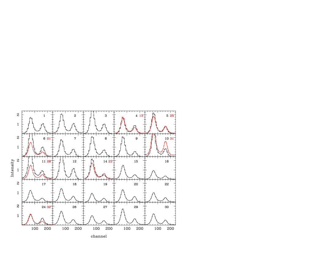
the number of scanning steps. Figure 1 shows the profiles
observed in the 25 fields.
The observing conditions were fairly
good, with some faint cirrus clouds on the nights of November 8th,
and 10th to the 13th. Only two exposures had to be cut because of heavy
clouds (number 14 and 25 in Table 2),
and the corresponding fields were re–observed
in good conditions with the 2h exposure time
currently adopted.
3 Data reduction
Basically, we have to analyze a short spectrum, 2.52 Å wide, which is the free spectral range of our Fabry-Perot interferometer. This means in fact that the positions of the lines are known modulo 2.52 Å, and that there is some overlapping of nearby lines since we select the lines to be analyzed through an 8 Å wide interference filter. For instance, the OH night sky line at 6568.78 Å appears closer to the H lines (geocoronal and Galactic) than it actually is, with an apparent separation of only 1 Å (6568.78 Å-6562.78 Å = 6.00 Å = 2 2.52 Å+ 0.96 Å), see Figure 2 (top panel).
The Galactic H emission is slightly separated from the geocoronal emission because of our motion with respect to the Galaxy. The motion of the Earth around the Sun and the motion of the Sun in the Galaxy were combined in such a manner that the separation between the two lines remained approximately constant, around 0.5 Å, along the bands of sky observed in November. As a result, the Galactic H emission should appear right between the two parasitic night sky lines (geocoronal H and OH). Its extraction is not easy, however, since it is typically 10 times fainter than the parasitic lines (see also Fig. 1 of Bartlett & Amram 1998), whose width (FWHM around 0.35Å) and shape (not far from gaussian) also tend to bury the signal in their wings.
First of all, to improve the signal–to–noise ratio and the spectral resolution, we selected a 30′ diameter disk centered on the interference rings observed in each field. This enables us to avoid the edges of the field where the interference rings are crowded and not sufficiently sampled by the pixel size of the image detector. The H emission profile obtained for each observed field is thus the addition of the profiles of all the pixels (about 31 000) found within from the center of the field.
To analyze this profile and extract the Galactic H emission, we must know precisely the shape of each line to be subtracted. The OH night sky line at 6568.78 Å is in fact the sum of two close components of the same intensity, one at 6568.77 Å and the other at 6568.78 Å. This fine structure can be neglected here, and the line may be considered as a single line. More complicated is the case of the geocoronal emission line, with not less than seven fine structure transitions. The two main components, produced by Lyman resonance excitation, are found at 6562.73 Å and 6562.78 Å, with a 2:1 ratio (Yelle & Roesler 1985). The resulting line center, at 6562.74 Å, is different from that in a discharge lamp (6562.79 Å), where all fine structure levels are excited. However, these two components proved insufficient when we decomposed our observed profiles, a residual remaining systematically at 6562.92 Å. This is due to cascade excitation which is particularly strong for the 7th component at 6562.92 Å (Nossal 1994). Although the percentage of cascade contribution is not accurately known, it proved satisfactory to use the Meier model cited in Nossal’s thesis, adding a component at 6562.92 Å with a 1:6 ratio compared with the brightest component at 6562.73 Å. To summarize, then, we decomposed the H geocoronal emission into three components : 6562.73 Å, 6562.78 Å (with intensity ratio 1:2) and 6562.92 Å (with intensity ratio 1:6).
The night sky line profiles are narrow and fairly well reproduced by the instrumental profile. This profile is obtained by scanning the emission line of a Neon lamp at 6598.95 Å during two hours.

We can thus subtract the OH line and geocoronal H components from our observed profile since we know their positions, the only free parameter being the intensity (remember, however, that the relative intensities of the three main components we considered for the geocoronal H line are kept fixed at 1, 1:2, 1:6). After subtraction of the night sky lines, a residual was found at the expected velocity for Galactic H emission, that is to say around zero in VLSR (radial velocity in the local standard of rest) and with the expected width, around 35 km , in good agreement with Reynolds’ (1990) results. Figure 2 shows an example of profile decomposition for one of our fields, together with a gaussian fit to the Galactic emission below. The width of the gaussian was left as a free parameter and adjusted automatically for the best fit. This width was typically found to lie between 25 an 50 km (see Table 2). For 7 out of our 32 observations, the signal–to–noise ratio was too faint for a good fit, and we imposed the average width (35 km ).
We scanned many fields with 48 steps, instead of the usual 24 steps, in order to check the interest of oversampling. Because of the Finesse of our Fabry-Perot interferometer (about 10 at H), the usual sampling criteria indicate that 24 scanning steps are sufficient to obtain profiles with the best achievable resolution. However, oversampling is sometimes necessary, especially when decomposing a profile into several close components. Indeed, we found no significant difference between the observations at 48 scanning steps and those at 24 steps, although the profiles drawn with 48 steps are smoother, precisely because of the better sampling.
The calibration in intensity was made by observing through the same instrument (although through a slightly redshifted H interference filter) the Hii region N11E in the Large Magellanic Cloud, for which an absolute calibration has been performed by Caplan & Deharveng (1985).
Let us note that we also used a rough method which produced nearly the same intensity variations. This method consists of assuming that the night sky lines are symmetric; then, taking into account the left wing of the geocoronal H line, which is contaminated by neither the Galactic emission nor the OH, one can infer that the right wing is its mirror image. Similarly, one considers the right wing of the OH night sky line, which is not contaminated by either Galactic emission or geocoronal H, and assumes that the left wing is its mirror image. The Galactic H emission is then deduced from the subtraction of these two symmetric lines. The results are not significantly different from the results obtained with our more sophisticated method.
4 Results
We find an intensity of Galactic emission in the observed bands, at and , varying between 0.2 R and 1.4 R (see Table 2), in good agreement with intensity values measured by Reynolds (1990) in the northern hemisphere far from the Galactic plane.
Figure 3 shows the measured intensity of Galactic H at declination °and °. The error bars are the average rms difference between the signal and the fitted gaussian, found to be 0.35 Rayleigh. We note that Reynolds (1990) quotes comparable uncertainties, Rayleigh.

To check the reproducibility of our observations, we observed seven fields twice. The differences in intensity we found for these fields vary by 40% in average, with just 0.4 Rayleigh as an average value, close to the uncertainty mentioned above. For the seven fields observed twice, the corresponding differences in intensity are (in % and in increasing order): 15, 21, 28, 43, 47, 52 and 79. The 43% difference may be easily explained by meteorologic effects, the lower intensity value having been obtained in bad conditions (the exposure had to be cut at 2640s because of clouds). The strong 79% difference may be explained, at least partially, by a drift of the field due to the loss of the guide star at mid–exposure. However, the remaining 47 and 52% differences are abnormally large and cannot be explained by observing conditions.
Figure 3 suggests that the overall variations are small and that the galactic H emission varies smoothly along the two bands of sky observed.
5 Discussion and conclusions
The goal of these observations was to constrain and quantify the possible Galactic free–free contamination of the SP91 and SP94 CMB results. The former consists of data taken along a strip at declination over a narrow range of frequencies centered on 30 GHz (K band), and which show a falling signal more characteristic of free–free emission than of the CMB. The SP94 scan being adjacent in declination, we also chose to observe along this band at , although these data were taken in both K and Q ( GHz) bands and show fluctuations consistent with a thermal spectrum (CMB).
The absolute intensity of the total emission over the observed bands is quite low (mean R and maximum R), with variations equal to our estimated uncertainty of R. As mentioned, this is consistent with previous work using both interferometers and narrow band filters. If we assume the WIM producing our signal is indeed at , then Eq. (4) indicates that it contributes at most K to the SP results in the K band. For comparison, the two largest fluctuations in SP91, those dominating the signal attain K, while the rms level seen in SP94 is K. A comparison of our results and the SP data sets is given in Figure 4, again using Eq. (4). It must be remembered that the SP points in this figure are really differences between fields adjacent on the sky, while the points represent absolute intensities at the given positions. Our results imply that, at a temperature of a few 104 K, the corresponding free-free emission is smaller than about 10 K at 30 GHz (K band), and hence does not significantly contaminate the SP experiments. It is worth mentioning, however, two possibilities which could lead to more important contamination of CMB signals despite low measured H intensities. Firstly, the above discussion assumes that the WIM does not have a higher temperature component. We note that even R variations, allowed at the –level, from a gas at K would produce fluctuations in K–band comparable to those observed in the SP data sets; the spectral information from the SP94 observations makes this seem unlikely, however. Secondly, it may well be that an important source of foreground to the contamination arises not from Bremsstrahlung, but from the rotational emission of very small spinning dust grains (Draine & Lazarian 1998). In this case, a correlation between the 30 GHz emission and the diffuse 12 m emission is expected. It remains to be seen whether these two effects will indeed be significant.

Acknowledgements
We thank the participants to the meeting organised in November 1995 by D. Valls–Gabaud and J.P. Sivan at the Observatoire de Haute Provence, for stimulating discussions.
References
- (1) Amram, P., Boulesteix, J., Georgelin, Y.M. et al., 1991, Messenger, 64, 44.
- (2) Bartlett, J.G. & Amram, P. 1998, in “Fundamental Parameters in Cosmology”, Moriond proceedings, in press, astro-ph/9804330
- (3) Caplan, J. & Deharveng, L. 1985, A&AS 62, 63
- (4) Draine, B.T. & Lazarian, A. 1998, ApJ 494, L19
- (5) Gaustad, J.E., McCullough, P.R. & Van Buren, D. 1996, PASP 108, 351
- (6) Gundersen, J.O., Lim, M., Staren, J., et al. 1995, ApJ 443, L57
- (7) Haslam, C.G.T., et al. 1981, A&A 100, 209
- (8) Jungman, G., Kamionkowski, M., Kosowsky, A. & Spergel, D.N. 1996, Phys. Rev. Lett. 76, 1007
- (9) Le Coarer, E., Amram, P., Boulesteix, J. et al. 1992, A&A 257, 389
- (10) Knox, L. 1995, Phys. Rev. D 52, 4307
- (11) Kogut, A., Banday, A.J., Bennett, C.L., Górski, K.M., Hinshaw, G. & Reach, W.T. 1996a, ApJ 460, 1
- (12) Kogut, A., Banday A.J., Bennett, C.L., Górski, K.M., Hinshaw, G., Smoot, G.F. & Wright, E.L. 1996b, ApJ 464, L5
- (13) Leitch, E.M., Readhead, A.C.S., Pearson, T.J. & Myers, S.T. 1997, ApJ 486, L23
- (14) Lineweaver, C.H., Barbosa, D., Blanchard, A. & Bartlett, J.G. 1997, A&A 322, 365
- (15) Netterfield, C.B. et al. 1997, ApJ 474, 47
- (16) Nossal, S. 1994, PhD. thesis, University of Wisconsin, Madison
- (17) Reich, P. & Reich, W. 1986, A&AS 63. 205
- (18) Reynolds, R.J. 1980, ApJ 236, 153
- (19) Reynolds, R.J. 1990, IAU symposium “The Galactic and Extragalactic Background Radiation”, Eds. S. Bower & C. Leinert, 157
- (20) Reynolds, R.J. 1992, ApJ 292, L35
- (21) Schuster, J., Gaier T., Gundersen, J., Meinhold P., Koch, T., Seiffert, M., Wuensche, C.A. & Lubin, P. 1993, ApJ 412, L47
- (22) Simonetti, J.H., Dennison, B. & Topasna, G.A. 1996, ApJ 458, L1
- (23) Smoot, G.F. et al. 1992, ApJ 396, L1
- (24) Smoot, G. 1998, astro-ph/9801121
- (25) Valls–Gabaud, D. 1998, PASA 15, 111
- (26) White, M., Scott, D. & Silk, J. 1994, ARA&A 32, 319
- (27) Wollack, E.J. et al. 1997, ApJ 476, 440
- (28) Yelle, R.V. & Roesler, F.L. 1985, J. Geophys. Res. 90, 7568
| Observations | Telescope | Marseille 36 cm |
| Location | La Silla | |
| Equipment | CIGALE Cassegrain focus | |
| Date | Nov 1996 | |
| Interference Filter | Central wavelength at 10C | 6566 Å |
| Transmission | 0.68 | |
| FWHM | 8 Å | |
| Calibration | H Comparison light | 6562.78 Å |
| Perot–Fabry | Interference order | 2604 @ 6562.78 Å |
| Free spectral range | 115 km s-1 | |
| Finesse at H | 10 | |
| Spectral Sampling | 24 Scanning steps | 0.105 Å (4.6 km s-1) |
| 48 Scanning steps | 0.052 Å (2.3 km s-1) | |
| Spatial Sampling | Total field | (256256 px2) |
| Useful circular field | ||
| Pixel size | ||
| Typical exposures times | Total exposure | 2 hours |
| Elementary scanning exposure time | 5 s per channel | |
| Total exposure time per channel | 300 s |
| Reference | Coordinates (2000) | Date | I(H) | FWHM | ||||
|---|---|---|---|---|---|---|---|---|
| number | s | mR | km s-1 | km s-1 | ||||
| 3 | 23h50m | 62° | Nov 5 1996 | 7200 | 24 | 1350 | 40 | 1 |
| 6 | 0h05m | 62° | Nov 6 1996 | 7200 | 24 | 1261 | 48 | 5 |
| 21 | 62° | Nov 11 1996 | 7200 | 48 | 901 | 31 | +1 | |
| 9 | 0h20m | 62° | Nov 7 1996 | 7200 | 24 | 628 | 72 | 2 |
| 12 | 0h35m | 62° | Nov 8 1996 | 7200 | 24 | 599 | 34 | 8 |
| 15 | 0h50m | 62° | Nov 9 1996 | 7200 | 48 | 422 | 27 | +4 |
| 18 | 1h05m | 62° | Nov 10 1996 | 7200 | 48 | 713 | 34 | 2 |
| 7 | 1h20m | 62° | Nov 6 1996 | 7200 | 24 | 1002 | 35 | +4 |
| 1 | 1h35m | 62° | Nov 4 1996 | 7200 | 24 | 723 | 34 | +10 |
| 2 | 1h50m | 62° | Nov 4 1996 | 7200 | 24 | 462 | 38 | +7 |
| 4 | 2h05m | 62° | Nov 5 1996 | 7200 | 24 | 705 | 35 | +12 |
| 13 | 62° | Nov 8 1996 | 7200 | 24 | 556 | 34 | +10 | |
| 10 | 2h20m | 62° | Nov 7 1996 | 7200 | 24 | 914 | 36 | +8 |
| 31 | 62° | Nov 15 1996 | 7680 | 48 | 1404 | 46 | +8 | |
| 16 | 2h35m | 62° | Nov 9 1996 | 7200 | 48 | 642 | 30 | +7 |
| 19 | 2h50m | 62° | Nov 10 1996 | 7200 | 48 | 403 | 26 | +13 |
| 20 | 3h05m | 62° | Nov 10 1996 | 7200 | 48 | 1065 | 34 | +13 |
| 17 | 3h20m | 62° | Nov 9 1996 | 7200 | 48 | 955 | 30 | +13 |
| 14 | 3h35m | 62° | Nov 8 1996 | 2640 | 24 | 777 | 31 | +14 |
| 23 | 62° | Nov 11 1996 | 7200 | 48 | 1353 | 35 | +11 | |
| 11 | 3h50m | 62° | Nov 7 1996 | 7200 | 24 | 1077 | 35 | +13 |
| 28 | 62° | Nov 13 1996 | 7200 | 48 | 566 | 34 | +15 | |
| 8 | 4h05m | 62° | Nov 6 1996 | 7200 | 24 | 1051 | 29 | +10 |
| 5 | 4h20m | 62° | Nov 5 1996 | 7200 | 24 | 1065 | 46 | +14 |
| 25 | 62° | Nov 12 1996 | 6960 | 48 | 905 | 28 | +11 | |
| 22 | 1h35m | 63° | Nov 11 1996 | 7200 | 48 | 391 | 28 | +6 |
| 26 | 1h50m | 63° | Nov 13 1996 | 7200 | 48 | 1399 | 38 | 0 |
| 27 | 2h05m | 63° | Nov 13 1996 | 7200 | 48 | 949 | 29 | +7 |
| 29 | 2h20m | 63° | Nov 14 1996 | 7200 | 48 | 189 | 34 | 6 |
| 24 | 2h35m | 63° | Nov 12 1996 | 7200 | 48 | 310 | 26 | +1 |
| 32 | 63° | Nov 15 1996 | 7200 | 48 | 524 | 34 | +12 | |
| 30 | 2h50m | 63° | Nov 14 1996 | 7200 | 48 | 787 | 28 | +3 |