The ionizing stars of extragalactic H II regions

Abstract

Medium-resolution spectra from 3650 Å to 10,000 Å are presented for 96 giant H II regions distributed in 20 spiral galaxies. In order to interpret the data, we have calculated two separate grids of photoionization models, adopting single-star atmospheres (Kurucz) and star clusters synthesized with different Initial Mass Functions (IMFs) as ionizing sources. Additional models were computed with more recent non-LTE stellar atmospheres, in order to check the effects of different stellar ionizing fluxes. We use the radiation softness parameter $\eta\prime$ = ([OII]/[OIII])/([SII]/[SIII]) of Vílchez and Pagel to test for a metallicity dependence of the effective temperatures of the ionizing stars. Our results are consistent with a significant decrease in mean stellar temperatures of the ionizing stars with increasing metallicity. The magnitude of the effect, combined with the behavior of the He I $\lambda$5876/H$\beta$ ratio, suggest a smaller upper mass limit for star formation at abundances higher than solar, even when considering the effects of metallicity on stellar evolution and atmospheric line blanketing. However, the exact magnitudes of the stellar temperature and IMF variations are dependent on the choice of stellar atmosphere and evolution models used, as well as on uncertainties in the nebular abundance scale at high metallicities.

Our results also constrain the systematic behavior of the ionization parameter and the N/O ratio in extragalactic H II regions. The observed spectral sequences are inconsistent with current stellar evolution models which predict a luminous, hot W-R stellar population in evolved H II regions older than 2–3 Myr. This suggests either that the hardness of the emitted Lyman continuum spectrum has been overestimated in the models, or that some mechanism disrupts the H II regions before the W-R phases become important.

Accepted for publication in the Astrophysical Journal

1 INTRODUCTION

Giant extragalactic H II regions are ionized by the massive stars of their young embedded clusters, and as such provide powerful tools for measuring the chemical composition of the interstellar medium and for understanding the massive stellar populations in external galaxies (see reviews by Shields 1990, Kennicutt 1991, Stasińska 1996). Evidence for abundance gradients across the disks of spiral galaxies was presented by Searle (1971), following pioneering work by Aller (1942) on the radial trends of emission-line ratios. The excitation of H II regions, measured by the ratios [OIII]$\lambda\lambda$4959,5007/H$\beta$ and [OIII]

Subsequent efforts were concentrated on quantifying this general picture, with the calculation of extensive grids of single-star photoionization models. Most authors confirmed the increase of $T_{*}$ with decreasing abundance (Stasińska 1980, Campbell, Terlevich & Melnick 1986, Vílchez & Pagel 1988), together with a possible increase in the ionization parameter (Campbell 1988). On the other hand Evans & Dopita (1985) argued that the available data on the trends in the emission-line ratios were consistent with a single ionizing temperature ($\simeq 41,500$ K) and a varying nebular geometry and ionization parameter. As the controversy is not completely settled, the presence of a $T_{*}$ gradient still needs to be clearly established and quantified, over the full range of abundances observed in spirals.

The fundamental question remains whether these apparent changes in $T_{*}$ are due to systematic variations in the Initial Mass Function (IMF) with metallicity and/or galaxy type. Abundance effects on either the upper mass limit (Shields & Tinsley 1976) or the slope of the IMF (Terlevich 1985) have been proposed. However, several other mechanisms have been suggested, including increased stellar line blanketing (Balick & Sneden 1976) or internal dust absorption (Sarazin 1976) with metallicity. Modern stellar evolution models (e.g., Maeder 1990) predict a softening of the stellar ionizing spectra with increasing abundance. The consequence for H II region models is a natural decrease of $T_{*}$, making the varying IMF hypothesis less compelling, as shown by McGaugh (1991). Moreover, the introduction of cluster photoionization models, in which the single star is replaced by an evolving stellar cluster as the ionizing source, has produced results which are consistent with a universal IMF (García-Vargas, Bressan & Díaz 1995, Stasińska & Leitherer 1996).

In this paper we re-examine the evidence for $T_{*}$ and IMF gradients, using new spectra of 96 H II regions in 20 galaxies over the 3650–10,000 Å range. This work extends previous large surveys of H II region spectra in spiral disks, including those of McCall, Rybski & Shields (1985), Vila-Costas & Edmunds (1992), Oey & Kennicutt (1993) and Zaritsky, Kennicutt & Huchra (1994). The main addition of the present work is the inclusion of data for the near-IR [SIII]$\lambda\lambda$9069,9532 lines, which allows measurement of the radiation softness parameter $\eta\prime$, directly related to the ionic fraction ratio $\eta$ = (O⁺/O⁺⁺)/(S⁺/S⁺⁺), introduced by Vílchez and Pagel (1988) as a $T_{\!\!\em eff}$ sensitive parameter. This paper extends to a large H II region sample the $\eta\prime$ method, which so far has been applied to studies of a few H II regions in individual galaxies. When combined with the empirical abundance indicator $R_{23}$= ([OII] + [OIII])/H$\beta$ (Pagel et al.1979) and an extensive set of nebular models we can simultaneously constrain the metallicity, the effective temperature and the ionization parameter (Díaz et al.1987, Vílchez et al.1988, Díaz et al.1991). A companion paper presents detailed modeling of 40 H II regions in one galaxy (M101), with emphasis on the $T_{*}$ gradient in a homogeneous sample of H II regions (Garnett & Kennicutt 1998). In the present work we examine a larger galaxy sample, spanning a wide range of abundance, with two main goals: to study the relationship bewteen $T_{*}$ and the gaseous abundance, and to derive constraints on IMF variations with metallicity. For this purpose, photoionization models including as ionizing source either an evolving star cluster or a single stellar atmosphere are computed. The new H II region sample is presented in § 2, and the nebular model grid is described in § 3. In the following sections we discuss our main results: systematics of H II region spectra and physical conditions (§ 4), evidence for a $T_{*}$ gradient (§ 5), and consequences for the upper IMF (§ 6). We summarize the main results in § 7. As a quick reference a list of abbreviations and symbols used is provided in Table 7.

2 OBSERVATIONS AND DATA REDUCTION

2.1 Sample

The galaxy sample (Table 7) spans the Hubble sequence from type Sa to type Sm, and should therefore provide good indication of trends of star forming region properties with morphological type. The H II regions cover a wide range in excitation, and their chemical abundance varies from Z $\simeq$ 0.2 ${\rm Z_{\odot}}$ to above solar (the lower limit is set by abundance determinations found in the literature for a few of the most metal-poor objects). Nearly all of the observations discussed here are new to this work, and were obtained during several runs in 1988-1992 on the Multiple Mirror Telescope (MMT) and the Steward Observatory 2.3m Telescope; the few exceptions are indicated in Table 7. The main observational material (redwards of H$\beta$) consists of spectra obtained with the MMT Red Channel Spectrograph with an echellette grating. Most of the blue spectra (which include the [OII] $\lambda$3727 line) were obtained at the MMT as part of the survey by Oey & Kennicutt (1993). Blue data for a few individual objects were drawn from the literature (McCall et al.1985, Zaritsky et al.1994, and Dufour et al.1980).

2.2 MMT Echellette Spectra

The Red Channel Spectrograph at the MMT was used in cross-dispersed mode to obtain spectral coverage from 4700 Å to 10,000 Å. This allowed the inclusion of all the main spectral features from H$\beta$ to [SIII] $\lambda\lambda$9069, 9532. In this observing mode a 2″ $\times$ 20″ slit was cross-dispersed into five orders, providing extended wavelength coverage at a resolution of 7-15 Å. The detector used was a Texas Instruments thinned 800$\times$800 device which, when binned 2$\times$2, provided a spatial scale of 0$\farcs$625 pixel^-1. Exposure times ranged from 5 to 40 min.

Data reduction included a few procedures particular to the echellette observations (see also Skillman & Kennicutt 1993 and Kennicutt & Garnett 1996). Standard star frames taken at low airmass were used to trace the aperture for each of the five orders and to remove the curvature introduced by the cross-disperser. Wavelength and flux calibrations were accomplished with HeNeAr lamp frames and observations of standard stars from Oke & Gunn (1983) and Massey et al.(1988), respectively. The calibrations were checked for internal consistency using lines in the overlap regions between adjacent orders. The residuals from the standard star fits indicate a typical accuracy of $\pm$0.05 mag rms or better in all orders except the reddest one ($\lambda$ $>$ 8000 Å). Here the water absorption features in the near-IR introduce a larger uncertainty in the flux calibration. The extinction was then modeled as a function of wavelength by tracing the absorption features observed in the standard star spectra. This procedure satisfactorily removes most of the unwanted telluric features around the [SIII] $\lambda\lambda$9069, 9532 lines, as indicated by the mean observed $\lambda$9532/$\lambda$9069 ratio = 2.47 $\pm$ 0.05 (the theoretical value is 2.44). Nevertheless we attach a conservative uncertainty of $\pm$20% to the [SIII] fluxes (see Kennicutt & Garnett 1996). One-dimensional spectra were extracted with variable apertures, typically eight arcseconds, but dependent on the seeing and the size of the objects, centered on the peak of the H$\alpha$ emission line. Care was taken to match as closely as possible the regions sampled in the blue spectra.

2.3 Blue Spectra

Coverage of the 3650–5100 Å spectral range was obtained with two different instruments and setups. The majority of our targets in early-type galaxies were observed with the Red Channel CCD spectrograph on the MMT and a slit size of 2″ $\times$ 180″. These observations have been described in detail by Oey & Kennicutt (1993) in their project on abundances in early-type galaxies. However, new one-dimensional extractions were made, to match those of the red echellette spectra.

Additional objects (marked $90^{\prime\prime}$ in Table 7) were observed with the B&C spectrograph at the Steward Observatory 2.3m telescope. Observations were made with a 600 groove mm^-1 grating blazed at 3568 Å, providing 9 Å resolution with a 4$\farcs$5 $\times$ 180″ slit. Standard reduction procedures for these long-slit data were followed. The H II regions in three galaxies (M31, M33 and NGC 2403) were observed in the red using a 300 groove mm^-1 grating blazed at 6690 Å, and providing 20 Å resolution with the 4$\farcs$5 slit. These data provided a check on the corresponding MMT echellette spectra. Blue data for NGC 628, NGC 2403, NGC 3521 and NGC 5236 were taken from the literature, with references given in Table 7.

2.4 Analysis of Spectra

The emission line fluxes for the atomic transitions of interest were measured with the IRAF task SPLOT, by integrating over the line profiles. We assumed a stellar underlying continuum Balmer absorption equivalent width of 2 Å, the mean value found by McCall et al.(1985) in their H II region sample, and calculated the reddening with the H$\alpha$/H$\beta$ and H$\beta$/H$\gamma$ ratios, assuming Case B recombination ratios for an electron temperature of 10,000 K and density of 100 cm^-3 (Osterbrock 1989). Table 7 lists the measured fluxes, corrected for reddening, for the most important emission lines, as well as offsets in arcseconds from the galaxy nucleus. Uncertainties in line fluxes were derived following the procedure described in Kennicutt & Garnett (1996), who analyzed H II region spectra in M101 taken with the same setup as the observations discussed in this work. The quoted errors were calculated by adding in quadrature the contributions from the statistical noise, the calibration ($\pm 3$%), the flat fielding ($\pm 1$%), the relative scaling of the echellette orders ($\pm 4$%) and the uncertainty in the reddening corrections. A 20% uncertainty was assigned to the combined [SIII] $\lambda\lambda$9069, 9532 flux, as described earlier.

We performed a few tests in order to check the quality of the data. As mentioned above the observed values of the [SIII]

3 PHOTOIONIZATION MODELS

In order to interpret the emission-line data for our H II regions, a set of nebular models was calculated with the CLOUDY program (Ferland et al.1998; Ferland 1996), version 90.01. Details about the models and more extensive results can be found in Bresolin (1997).

Given the spectral energy distribution (SED) of the ionizing source, the ionizing photon luminosity, the chemical composition and the geometry of the gas, the code solves for the ionization and thermal equilibrium of the nebula. A relevant aspect of the version of the code used for these calculations is the inclusion of Opacity Project data (Seaton et al.1994). For our models the important change (approaching a factor of two) with respect to previous versions of the code regards the O⁺ photoionization cross section, which no longer shows a jump at the 2s – 2p edge. A further change in the O⁺ - O⁺⁺ balance is caused by new collision strengths for some O⁺⁺ lines. To assess the effect of the new atomic data on the final results, a set of single-star photoionization models (described in the next section) were calculated with an older version of CLOUDY ($v.\;84.12$), and compared with the results of $v.\;90.01$. The newer version predicts an average decrease of the [OII] line intensity of approximately 20%, mostly counterbalanced by an increase in the [OIII] emission. The corresponding effect on the empirical abundance indicator $R_{23}$ translates into an approximate 0.025 dex increase in the (O/H) abundance scale, based on the calibration given by Zaritsky et al.(1994).

For the remainder of this section the input parameters of the models will be described; the relevant model results will be illustrated in § 4

3.1 Input Parameters

3.1.1 Spectral Energy Distributions

As mentioned above, two different SEDs were considered as the ionizing source of the nebulae. The single-star models are simpler cases in principle, as they can be interpreted in terms of one parameter, $T_{*}$, which is a function of the hardness of the output ionizing spectrum. On the other hand, cluster models contain information on the mass function and the temporal evolution of the ionizing clusters.

For single-star models, the line-blanketed LTE Kurucz (1992) stellar atmospheres, which include the effects of bound-free opacity from heavy elements, were adopted for consistency with the cluster models. The $\log g=5$ atmospheres were chosen, in order to circumvent problems of non-convergence of the hydrostatic LTE atmospheres at low stellar surface gravity. The metallicity was varied in accordance with the gas abundance. Nebular models were calculated at Z = 0.25 ${\rm Z_{\odot}}$, ${\rm Z_{\odot}}$ and 2 ${\rm Z_{\odot}}$, and for $T_{\!\!\em eff}$ = 37,500 K, 40,000 K, 45,000 K, 50,000 K and 60,000 K. The sensitivity of the results to the choice of stellar atmosphere models will be discussed later.

An alternative approach is to calculate SEDs for star clusters with different IMFs. This method was applied by McGaugh (1991) for zero-age clusters, and taking into account the temporal evolution of the clusters by García-Vargas & Díaz (1994), Cerviño & Mas-Hesse (1994), García-Vargas et al.(1995), and Leitherer & Heckman (1995).

We adopted the SEDs calculated by Leitherer & Heckman (1995), as presented in Leitherer et al.(1996a). These SEDs were also calculated for different metallicities (those at 0.25 ${\rm Z_{\odot}}$, ${\rm Z_{\odot}}$ and 2 ${\rm Z_{\odot}}$ are relevant to the present work) and IMFs ($\alpha~{}=~{}2.35$ and M_up = 100 ${\rm M_{\odot}}$, $\alpha~{}=~{}2.35$ and M_up = 30 ${\rm M_{\odot}}$, $\alpha~{}=~{}3.35$ and M_up = 100 ${\rm M_{\odot}}$, where the IMF is given by $dN/dm~{}\propto~{}m^{-\alpha}$ between M${}_{low}=1$ ${\rm M_{\odot}}$ and M_up), at 1 Myr intervals from 1 to 25 Myr. The stellar models of Maeder (1990) and Maeder & Meynet (1988) were used for the synthesis, together with Kurucz’s (1992) atmospheres, supplemented by the non-LTE models of Schmutz, Leitherer & Gruenwald (1992) for stars with strong winds. We used the results of both the instantaneous burst case, in which star formation occurs over a timescale short compared to the age of the model, and the continuous star formation case (star formation constant with time). We considered ages from 1 to 6 Myr, since at later times most clusters would lack the necessary ionizing luminosity to produce an H II region (García-Vargas & Díaz 1994). For further details on the cluster SEDs, the reader is referred to the original papers.

3.1.2 Nebular Gas Parameters

The abundance of the gas has been made consistent with the metallicity of the ionizing stars. The solar elemental abundances are adopted as defined in Grevesse & Anders (1989). To take into account depletion of refractory elements onto dust grains, the elements Mg, Al, Ca, Fe, Ni and Na were depleted by a factor of 10, and Si by a factor of two, relative to the solar abundance (consistent with Garnett et al.1995, Garnett & Kennicutt 1998). The He abundance was scaled according to Y = Y_p + ($\Delta$Y/$\Delta$Z) Z, where Y $=4y/(1+4y)$, $y$ = He/H by number, and Z is the metallicity (${\rm Z_{\odot}}$ = 0.02). We have adopted Y${}_{p}=0.23$ (Pagel et al.1992), and $\Delta$Y/$\Delta$Z=2.5. Table 7 summarizes the adopted solar composition, with the above-mentioned depletions taken into account.

The model geometry is spherical, with a constant gas density n = 50 cm^-3, and with a filling factor $\epsilon$ adjusted so as to obtain models with three different ionization parameters, $\log U=-2,-3$ and $-4$. The dimensionless ionization parameter $U$ is defined as

$$U=\frac{\mbox{$Q_{H^{0}}$}}{4\pi R_{s}^{2}nc}$$ (1)

where $Q_{H^{0}}$ is the number of hydrogen-ionizing photons (E $>$ 13.6 eV) emitted per second, R_s is the Strömgren radius, n is the hydrogen density and c is the speed of light. $U$ depends on the electron temperature, T_e, through the Strömgren radius dependence on the case B recombination coefficient $\alpha_{B}(T)$:

$$R_{s}=\left(\frac{3}{4\pi}\frac{\mbox{$Q_{H^{0}}$}}{\alpha_{B}n^{2}\epsilon}\right)^{1/3}$$ (2)

with $\alpha_{B}(T)\propto T_{e}^{-1}$, so that we can rewrite

$$U=A(\mbox{$Q_{H^{0}}$}n\epsilon^{2})^{1/3}$$ (3)

with $A\propto T_{e}^{-2/3}$. We had therefore to iterate a few times, from an initial guess for the filling factor, to obtain the desired $\log U$. A few models were calculated for n = 10 cm^-3 and n = 150 cm^-3, to estimate gas density effects, which are quite strong at higher metallicities (Díaz et al.1991).

We fixed the total number of ionizing photons to $Q_{H^{0}}$ = 10⁵¹ s^-1, the equivalent of $\sim$90 O7 V stars (Vacca 1994), and representative of bright extragalactic H II regions. The exact value of $Q_{H^{0}}$ is of no practical importance, since it acts as a scaling factor, and models with a given ionizing spectrum shape and differing $Q_{H^{0}}$, n and $\epsilon$, but with the same $U$ are homologous, producing the same emission-line relative strengths (as long as the density is below the critical limit for collisional de-excitation) and the same nebular ionization structure. The corresponding initial cluster masses are large enough ($>1\times 10^{4}$ ${\rm M_{\odot}}$) that our models remain unaffected by the stochastic effects described by García-Vargas & Díaz (1994) and Cervińo & Mas-Hesse (1994). We also emphasize that CLOUDY computes nebular models in which a compact ionizing source lies at the center of a spherically symmetric gas distribution. We do not expect significant changes in the case of a more extended ionizing source (e.g. a loose OB association) as long as it remains unresolved by the spectrograph slit, since the emission-line properties are controlled by a quantity integrated over the volume of the nebula (the ionization parameter).

All of our models are ionization-bounded, with the calculation stopped at a gas temperature of 100 K (the optical opacity of the gas is negligible even at a much higher temperature). The models include a 30 km s^-1 turbulent velocity term, consistent with observed linewidths of giant H II regions (Arsenault & Roy 1988). This additional velocity field increases the line widths (already broadened by thermal motions), affecting the energy budget of the H II regions. A cooling of the nebulae results through infrared fine-structure lines, which can become optically thin as a result of the line broadening. The effects of dust have not been taken into account, except for the depletion of refractory elements.

For the interested readers, the results of our models can be retrieved, in the form of tables and diagnostic diagrams, by anonymous ftp, by contacting the first author.

4 RESULTS

A useful quantity that can be readily estimated from the stellar atmosphere SEDs is the ratio of He⁰ ionizing photons ($\lambda\leq 504$ Å) to H ionizing photons ($\lambda\leq 912$ Å), $Q_{He^{0}}$/$Q_{H^{0}}$, for each metallicity and $T_{\!\!\em eff}$. For a particular atmosphere model, this ratio describes the hardness of the radiation field, and has been used to define an equivalent ionizing temperature, T_eq, as the $T_{\!\!\em eff}$ of a star whose SED produces a given $Q_{He^{0}}$/$Q_{H^{0}}$ (Mas-Hesse & Kunth 1991, García-Vargas & Díaz 1994). A calibration of this ratio for the Kurucz (1992) $\log g=5$ atmospheres is given in Table 7. Clearly the radiation field becomes harder as $T_{\!\!\em eff}$ increases, and with lowering metallicity at a fixed temperature. The sensitivity to abundance is largest at high temperatures, becoming progressively smaller at lower $T_{\!\!\em eff}$. The abundance effects can be quite important, since they can be equivalent to a change in $T_{*}$ of as much as 10,000 K between 2 ${\rm Z_{\odot}}$ and 0.1 ${\rm Z_{\odot}}$.

The $Q_{He^{0}}$/$Q_{H^{0}}$ ratios for the cluster models are shown in Table 7. As pointed out by García-Vargas et al.(1995), the evolution of T_eq is non-monotonic at higher metallicities, due to the hardening of the radiation after the predicted W-R phase sets in. This effect disrupts the T_eq – metallicity relationship valid for ages smaller than about 3 Myr, for which T_eq drops by 5000-6000 K (from 50,000 to 45,000 K at t = 1 Myr) between 0.1 ${\rm Z_{\odot}}$ and 2 ${\rm Z_{\odot}}$. The presence of the W-R stars strongly affects the results 2-3 Myr after the burst of star formation. The effect is stronger with increasing metallicities, because of the larger number of W-R stars produced.

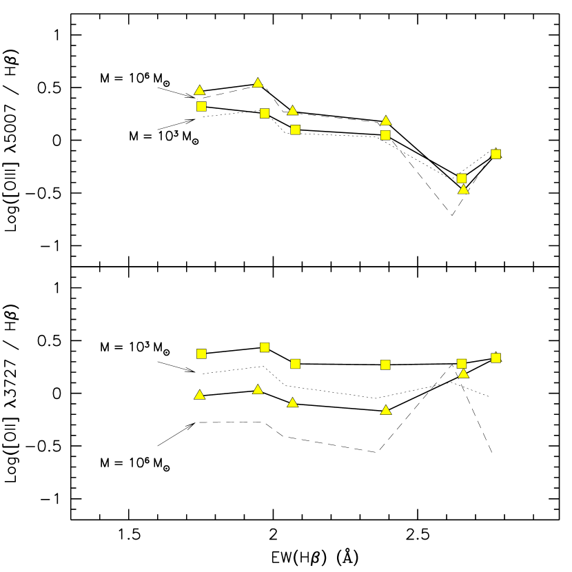
Figure 2: Comparison with the models of Stasińska & Leitherer (1996). The latter are shown for an ionizing cluster mass M = 10³ and M = 10⁶ ${\rm M_{\odot}}$, with dotted and dashed lines, respectively. Our models for $\log U\,=\,-2$ and $\log U\,=\,-3$ (calculated for n = 10 cm^-3) are shown by the continuous lines connecting triangle and square symbols, respectively. All models are for solar composition. (Top) [OIII]$\lambda$5007/H$\beta$ vs EW(H$\beta$). (Bottom) [OII]$\lambda$3727/H$\beta$ vs EW(H$\beta$).

A direct comparison of our model results with those of other authors is made difficult by the use of different input parameters and photoionization codes. However, a small set of solar composition models, with n = 10 cm^-3, was compared to the models by Stasińska & Leitherer (1996). The latter were calculated with the code PHOTO (Stasińska 1990) and the same cluster SEDs used in the present work, for different cluster masses. Due to the evolution of the massive stars, the total ionizing luminosity (and hence the ionization parameter) is a function of cluster age, while in our models we have kept it constant, in order to set the ionization parameter to the desired values. The Stasińska & Leitherer models for cluster masses M${}_{*}=10^{3}$ and 10⁶ ${\rm M_{\odot}}$ and ages between 1 and 6 Myr (M_up = 100 ${\rm M_{\odot}}$) have an ionization parameter in the range –1.6 to –2.9, and can therefore be compared to our $\log U\,=\,-2$ and –3 models. Figure 2 shows the comparison regarding [OIII]

4.1 Ionization Parameter

The model results indicate that the ionization parameters adopted for the models well bracket our data, which are clustered around $\log U=-3$. This is demonstrated in Figure 3, which plots [SII]$\lambda\lambda$6717,6731/[SIII]$\lambda\lambda$9069,9532 vs the abundance parameter $R_{23}$ for our sample. Díaz et al.(1991) gave a calibration of $U$ in terms of this ratio, which has been refined by Garnett & Kennicutt (1998) to include the small metallicity dependence. Similarly we have used a surface fit to our models in order to derive the following relation:

$$\log U=(-3.35\pm 0.04)-(1.54\pm 0.05)\log([SII]/[SIII])-(0.08\pm 0.06)\log(R_{23})$$ (4)

According to this calibration and the observed [SII]/[SIII] ratios the ionization parameter in our sample is in the range $\log U=-3\pm 0.6$. The comparison of the models with the observations suggests also that for the most metal-poor objects ($\sim$ 0.2 ${\rm Z_{\odot}}$) the ionization parameter is about 4 times larger than for H II regions around the solar metallicity. This finding is in agreement, at least qualitatively, with previous investigations of H II galaxies (Campbell 1988, Stasińska & Leitherer 1996).

4.2 The N/O abundance ratio

The [NII]/[OII] model sequences do not reproduce the observations at low abundances when a constant N/O ratio is adopted. The actual data show weaker [NII] lines relative to [OII] when compared to the theoretical values. Theory and observations could be reconciled by considering a metallicity-dependent N/O ratio. Evidence for such an effect in spirals has already been shown by several authors (e.g. McCall et al.1985, Fierro, Torres-Peimbert & Peimbert 1986, Díaz et al.1991, Garnett & Kennicutt 1998), but there is no general agreement on the functional relation between N/O and O/H, if it exists at all (different spirals having possibly different N/O gradients, Henry & Howard 1995; these authors, however, neglected primary nitrogen in deriving their gradients). In low-abundance irregular galaxies the N/O ratio is found to be independent of O/H (Garnett 1990), supporting the idea of a primary origin for nitrogen at low metallicity: nitrogen is produced out of C and O synthesized during the evolution of stars. An abundance-sensitive N/O ratio would imply the presence of a secondary component, that is N produced by C and O already present in stars at their birth. The situation is less clear for S/O, for which the existence of a O/H dependence is uncertain (for example, see contradicting results in Díaz et al.1991 and Garnett 1989). To represent a secondary component superposed on a primary component for N in spiral galaxies, a few models were calculated assuming the following relations (Garnett & Kennicutt 1998):

$$\log N/O=-1.5+(\log O/H+3.7)\qquad(\log O/H>-3.7)$$ ()

$$\log N/O=-1.5\phantom{+(\log O/H+3.71)}\qquad(\log O/H<-3.7)$$ ()

The results (Fig. 4) are in much better agreement with the observations, lending more credibility to the presence of a secondary component for nitrogen in spiral galaxies. The models can now reproduce the steepening of the [NII]/[OII] vs $R_{23}$ relation that occurs in the data at Log $R_{23}$ $>~{}$0.5. The main secondary effect of the abundance-dependent N/O ratio is a shift of the 2 ${\rm Z_{\odot}}$ models to lower $R_{23}$ values, due to the increased cooling of the nebulae caused by the larger abundance fraction of nitrogen. Models with a fixed, solar N/O ratio would therefore overestimate the metallicity for high-abundance objects. The models presented in this paper were calculated with a constant N/O ratio; however the effects of a variable ratio for all the diagnostics but those involving [NII] are, for all our purposes, marginal and limited to Z $>$ Z_⊙.

An important point to make about the [NII]/[OII] sequence is that it refers to 20 spiral galaxies of different Hubble type. The tightness of the sequence implies that the relation between N/O and O/H is similar for all these galaxies, whatever the exact functional form might be. While for a few individual galaxies (e.g. M33, see Vílchez et al.1988, or M81, see Garnett & Shields 1987) a N/O gradient seems not to be required, a ‘universal’ abundance-dependent N/O ratio seems to be necessary to explain the bulk of our observations.

4.3 The H$\beta$ Equivalent Width

Bresolin & Kennicutt (1997) studied the distribution of the H$\alpha$ equivalent width [EW(H$\alpha$)] of H II regions in ten galaxies of different Hubble type to test the idea that different upper mass limits of the IMF could be responsible for the changes in star forming region properties as a function of morphological type. The photometrically-determined EW(H$\alpha$) values showed no dependence on Hubble type. The distribution of the equivalent width of H$\alpha$ and H$\beta$ for our H II region sample confirms this result. Since the equivalent width of the Balmer emission lines is a measure of the ratio of the number of hot, massive stars (producing the emission line flux through ionization of the nebula) to the total number of stars (producing the continuum), our result points toward the invariance of the IMF across the morphological sequence.

The data show a dependence of EW(H$\beta$) on metallicity, with a large scatter, likely due to an age spread in the H II region sample. A similar behavior was already measured by Searle (1971) on a small sample of H II regions in M101. This result was interpreted by Shields & Tinsley (1976) as evidence for a gradient in the temperature of the hottest exciting stars, which in turn led them to hypothesize an abundance-dependent upper mass limit for star formation. The photoionization models, however, fail to reproduce the observed sequence of EW(H$\beta$) vs $R_{23}$. It is a well-known fact that the observed EW(H$\beta$) values of extragalactic H II regions are much lower than the theoretical predictions. The usual interpretation is that an underlying population of stars older than the ones responsible for the ionization of the nebulae is contributing to the stellar continuum, thus diluting the ionizing radiation and reducing the equivalent width (McCall et al.1985). Diaz et al.(1991) proposed the coexistence of stellar clusters of different ages within giant H II regions, as suggested by spatially resolved observations (Skillman 1985, Díaz et al.1987). Internal extinction due to dust which would affect the nebular lines, but not the continuum, has been proposed as an alternate solution (Mayya & Prabhu 1996, García-Vargas et al.1997). The dependence of EW(H$\beta$) on both cluster age and upper IMF, combined with the problem just described, make it difficult to derive a $T_{\!\!\em eff}$–Z relationship from EW(H$\beta$). Therefore we will not attempt to use the observed EW(H$\beta$) to infer a $T_{*}$ gradient.

4.4 Cluster Ages

A $T_{*}$-metallicity relation is expected for young clusters (1-2 Myr after initial burst), as a result of metallicity-dependent effects on the stellar output flux. The onset of the W-R phase for massive stars which occurs after 2-3 Myr of the initial burst would disrupt this correlation for a mixed-age sample of clusters, as shown by García-Vargas et al.(1995). The observation of a $T_{*}$ gradient in our sample of H II regions (§ 5) would therefore imply, if theory and models are correct, that an age limit exists. Interestingly, this would agree with the fact that the instantaneous burst cluster models are only able to reproduce the data for young cluster ages (t $<$ 3 Myr). The theoretical predictions diverge considerably from the observations at later times. This does not exclude the likely presence of older H II regions in our sample, but the average of the H II region sequences is best reproduced by the 1 and 2 Myr models, when we make the assumption that the ionizing sources are single population clusters. As an example, we show the diagnostic diagrams which summarize the model results for [OII]/[OIII] vs $R_{23}$ in Figure 5. Here the data (solid dots) are compared with the models, calculated for three different values of the ionization parameter and for three different cluster IMFs, as explained in § 3. It can be seen that the hardening of the stellar radiation predicted after 2 Myr from the initial burst produces line ratios which cannot in general be reconciled with the observations (see also Fig. 13). There remains the possibility that the nebular models are at fault, even though state-of-the-art codes and models have been adopted for both the gaseous and the ionizing source treatment. Alternatively some of the predictions of the stellar evolutionary models could be incorrect. In short, our results imply that either the current evolution models overpredict the hardness of the emitted Lyman continuum spectrum, or that some physical mechanism, such as disruption by stellar winds and/or supernova explosions, prevents us from observing H II regions older than a few million years.

The continuous star formation cluster models often provide as good a fit to the observations as the single-age burst models. Although most published photoionization models are based on instantaneous burst models, this suggests that continuous models should also be considered as valid alternatives. Star formation extending over time (an age spread of a few Myr), as in the case of individual star clusters formed in subsequent bursts, but close enough to remain unresolved by the spectrograph slit, is a scenario that deserves further investigation. This is the case of 30 Dor, whose central ionizing cluster has an age of $\sim$3 Myr; there is however evidence for previous episodes of star formation, as indicated by the presence of supergiants (Walborn 1991). These components of different age are spatially resolved, but they would not be if 30 Dor were at a much larger distance. Recent work (García-Vargas et al.1997, Gonzáles-Delgado et al.1997) indicates the coexistence of young ($\sim$3 Myr) and old ($\sim$8 Myr) components in individual starbursts, supporting the idea of an age spread, and suggesting star formation in multiple, subsequent bursts as a likely mechanism in giant H II regions.

5 TEMPERATURE OF THE IONIZING STARS

Shields & Searle (1978) were the first to point out the importance of the [SIII]$\lambda\lambda$9069,9532 lines to constrain the ionization structure of H II regions in the absence of temperature-sensitive lines, since sulfur is an effective coolant through these near-IR forbidden lines and the fine-structure lines at 19 and 33 $\mu$m. Mathis (1982, 1985) later introduced a method to determine the relative effective temperature scale, based on S⁺/S⁺⁺ and O⁺/O. The use of ratios of ionic stages of the same element makes this method almost independent of nebular abundance. However, absolute values of $T_{*}$ are much more difficult to obtain, due to the dependence on the stellar atmospheres adopted for the nebular models. Besides, there is a saturation effect for very hot stars, so that the method becomes less useful at high temperatures (Garnett 1989).

A ‘radiation softness’ parameter $\eta$ was introduced by Vílchez & Pagel (1988) as a modification of Mathis’ procedure, and defined as

$$\eta=\frac{\mbox{O${}^{+}$}/\mbox{O${}^{++}$}}{\mbox{S${}^{+}$}/\mbox{S${}^{++}$}}.$$ (6)

It is almost independent of ionization parameter, reddening, electron density and temperature. The observed quantity is given by

$$\eta\prime=\frac{\rm[OII]\mbox{$\lambda\lambda$}3726,3729\;/\;\rm[OIII]\mbox{$\lambda\lambda$}4959,5007}{\rm[SII]\mbox{$\lambda\lambda$}6717,6731\;/\;\rm[SIII]\mbox{$\lambda\lambda$}9069,9532.}$$ (7)

As a measure of the hardness of the radiation field, this parameter provides us with an indicator of the $T_{\!\!\em eff}$ of the exciting stars of H II regions. The large difference in the ionization potentials of O⁺ (35.1 eV) and S⁺ (23.2 eV) is responsible for the sensitivity of $\eta$ to the spectral energy distribution of the ionizing radiation. Spatially resolved observations of the Orion Nebula, NGC 604 in M33 and 30 Doradus in the LMC confirm the reliability of this method (Vílchez & Pagel 1988, Mathis & Rosa 1991), although Ali et al.(1991) questioned it on the basis of possible effects of dielectronic recombination on the sulfur lines (the relative coefficient has not been computed yet). Applications of the $\eta$ method to study the physical properties of extragalactic H II regions include the works of Díaz et al.(1987), Vílchez & Pagel (1988), Díaz et al.(1991) on the high-metallicity H II regions in M51, and Garnett & Kennicutt (1998) on a large sample of objects in M101.

There is a general agreement about the existence of a metallicity dependence of the hardness of the radiation for H II region ionizing clusters. For example, in a sample of high-excitation H II regions Stasińska (1980) found that $T_{\!\!\em eff}$ increases statistically with decreasing abundance. The same conclusion has been reached by studies of the generally metal-poor H II galaxies (Campbell et al.1986, Melnick 1992, Cerviño & Mas-Hesse 1994). Vílchez & Pagel (1988) confirmed this trend based on a compilation of H II region data from several authors. At any given abundance the spread in $T_{\!\!\em eff}$ typically amounts to $\sim$5,000 K, which can be due to several combined causes, such as evolutionary effects, uncertainties in the models, and differences intrinsic to the ionizing population. The methods used in these works were based on the determination of electron temperatures, mainly via the [OIII]

Different authors have instead debated over the cause of the $T_{*}$ gradient, whether it is a reflection of a change in the upper IMF (e.g. Campbell et al.1986), or simply an effect of stellar evolution at different metallicities (McGaugh 1991). To illustrate the latter, we show in Fig. 6 the metallicity–$T_{\!\!\em eff}$ relation predicted by the Geneva stellar evolutionary models for different stellar masses, and for ages of zero and one Myr (Schaerer et al.1993b, and references therein). For massive stars a decrease of the order of 5,000 K or more, up to $\sim$10,000 K, exists in the metallicity range 0.05 ${\rm Z_{\odot}}$ – 2 ${\rm Z_{\odot}}$. The effect is stronger at low abundance, where the gradient is steeper, which seems to be in agreement with H II region observations.

In the following we examine our data in search for variations of $T_{*}$ with abundance, by means of the analysis of the $\eta\prime$ parameter. Since our sample covers the range in metallicity from about 0.2 ${\rm Z_{\odot}}$ to above solar, we are able to extend previous work in order to check if the $T_{*}$ trend continues at higher abundances. However, as mentioned above, the expected change in this metallicity range is rather limited, making it more difficult to detect. The fact that at high abundance the modelling of H II regions becomes problematic (due also to the lack of electron temperatures, forcing us to use an empirical calibration for the metallicity) complicates the interpretation of the data. In addition, the dependence of the results on the stellar atmospheres adopted, and the sensitivity to the ionization parameter make the precise $T_{*}$ scale, and in part its gradient, model dependent.

5.1 $T_{*}$ gradient from single-star models

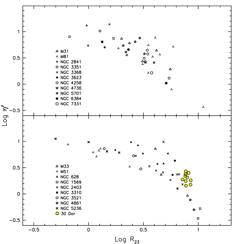
Figure 8: Identification of the H II region parent galaxies in the $\eta\prime$ – $R_{23}$ diagram. Early-type (Sa–Sb) and late-type (Sbc–Sm) spirals are shown in the upper and lower half of the figure, respectively. Spatially resolved observations of 30 Dor are included for comparison.

Figure 7 shows the $\eta\prime$ vs $R_{23}$ diagnostic diagram for our data and single-star models, and illustrates the main difficulties in deriving a $T_{*}$ gradient from $\eta\prime$. The main complications are its dependence on $R_{23}$ (at constant T and $U$) and the weaker sensitivity to $T_{*}$ in the high-$T_{*}$ range. Changes in the ionization parameter also have considerable effects on the results. We finally remind the reader about the rather mild $T_{*}$ dependence on metallicity which is expected when the abundance is larger than about half solar. The H II region parent galaxies are labeled in the $\eta\prime$ – $R_{23}$ plot of Figure 8, where the sample has been divided into early-type (Sa–Sb; upper panel) and late-type (Sbc–Sm; lower panel) spirals. We also include spatially resolved observations of the 30 Doradus nebula in the LMC by Kennicutt & French (Kennicutt et al., in preparation), which show that the dispersion in line ratios for a typical supergiant H II region is roughly of the same magnitude as the dispersion in the whole sample. When compared with the models of figure 7, this leads us to conclude that accurate $T_{*}$ determinations cannot be obtained through $\eta\prime$. The strength of the method lies in the possibility of detecting large-scale trends of $T_{*}$ in a large sample of high-abundance H II regions.

In order to simplify the interpretation of the data, in Fig. 9a we have divided the H II region data into two ionization parameter classes ($\log U$ above and below $-2.75$), according to the measured [SII]/[SIII] ratio and equation (4), and superposed the models calculated for $\log U=-2.5$ and $-3.0$ at various stellar effective temperatures for the Kurucz atmospheres. The comparison of the models with the observed sequence suggests a metallicity dependence of $T_{*}$, in the sense that the upper bound of $T_{*}$ shifts to lower temperatures at higher abundances, in a fashion similar to what Campbell (1988) noted for metal poor H II galaxies. Within our sample this effect is more easily seen in the high ionization parameter range ($\log U>-2.75$). Quantifying it is however much more difficult, and, as the bottom part of Fig. 9a shows, the models do not agree with all the observational data. This discrepancy was seen by, among others, Skillman (1989) and Garnett (1989), who pointed out that the S⁺/S⁺⁺ ratio is underpredicted (or O⁺/O⁺⁺ overpredicted) by nebular photoionization models. It has been suggested that the origin of the disagreement lies in the sulphur atomic parameters (Garnett 1989) or in density inhomogeneities of the nebular gas (Rosa 1993). Garnett (1989), after examining the effects of different stellar atmospheres on the model predictions for these two ionic ratios, concluded that only relative changes of $T_{*}$ can be inferred from $\eta$. Before reaching any conclusion on the existence of a $T_{*}$ gradient at high abundance we will also briefly consider the effects of changing the input stellar atmospheres, including the most recent, state-of-the-art hot star atmosphere models.

5.2 Effects of input stellar atmospheres on the interpretation of the $T_{*}$ gradient

The choice of stellar atmospheres, such as the widely used models by Mihalas (1972) and Kurucz (1979, 1992), is responsible for well-known differences in the predicted emission line ratios when computing H II region photoionization models (Skillman 1989, Evans 1991). These models have well-recognized inadequacies, namely the absence of line blanketing (Mihalas) or treatment of plane-parallel atmospheres in LTE (Kurucz). The inadequacy of these models for early-type stars derives from severe departures from LTE and the onset of radiation-driven stellar winds (Kudritzki & Hummer 1990, Kudritzki 1998). Enormous progress has been made in the last decade in stellar atmosphere modeling, in being able to treat theoretically the effects of departures from LTE, opacity from metal lines, stellar winds, and spherical extension on the computed hot star spectral energy distribution and ionizing flux (Gabler et al.1989, Najarro et al.1996, Schaerer et al.1996a,b). The modifications with respect to previous calculations are profound. For instance, the predicted flatter ionizing flux distribution in the He I continuum (below 504 Å) has already offered a solution for a long-lasting discrepancy between observations and nebular models regarding the intensity of the [NeIII] lines, severely underpredicted (up to a factor of 10 or more) when adopting the Kurucz atmospheres (Sellmaier et al.1996, Stasińska & Schaerer 1997). Our understanding of the stellar populations responsible for the ionization of extragalactic giant H II regions is also affected, as shown by the possible explanation of high-excitation nebulae in terms of ‘normal’ massive O stars, instead of more exotic ionizing sources (Gabler et al.1992).

Various predictions of the spectral energy distribution of hot stars are becoming available (Pauldrach et al.1994, Sellmaier et al.1996, Najarro et al.1996, Schaerer & de Koter 1997, Pauldrach et al.1998). While basically the same physical processes are taken into account, considerable differences exist in modeling techniques, for example in computing the occupation numbers for the different ions, so that different H II regions ionization structures would be predicted. While a detailed comparison is out of the scope of the present paper, we have computed nebular models based on stellar atmospheres different from Kurucz’s, in order to verify that the general, qualitative conclusions remain unchanged. We have therefore computed nebular models using the most recent early-type star atmospheres available: the CoStar models (Schaerer & de Koter 1997), available for two different metallicities (${\rm Z_{\odot}}$ and 0.2 ${\rm Z_{\odot}}$), and recent hydrodynamical non-LTE calculations of expanding atmospheres kindly made available to us by the Munich group (see Pauldrach et al.1998). The latter, too, were calculated for Z = ${\rm Z_{\odot}}$, 0.2 ${\rm Z_{\odot}}$. The 2 ${\rm Z_{\odot}}$ nebular models were computed with solar abundance stellar atmospheres. Additional models were computed with the Mihalas (1972) atmospheres, keeping the abundance of the stellar ionizing source fixed. All the remaining parameters were the same as described earlier for the Kurucz atmospheres.

Without discussing the different theoretical approaches, for which we refer the reader to the above-mentioned papers, or the apparent merits and faults of the atmosphere models used in this comparison, we present in Figs. 9b–9d the resulting models in the $\eta\prime$ – $R_{23}$ diagram, with the same partition of the data into two ionization parameter bins as in Fig. 9a. The figures demonstrate very clearly that the absolute $T_{*}$ scale greatly depends on the adopted input ionizing flux. It is particularly interesting that the two most recent non-LTE expanding atmosphere models give very different results in the lower $T_{\!\!\em eff}$ regime; future work on H II region modeling can in principle be very useful in solving these discrepancies. Concentrating however on the points in common, we find that all models are consistent with higher $T_{*}$ values ($\geq 50,000$ K) at the lowest abundances, while at high abundance $T_{*}$ levels off at a smaller value, between 35,000 K and 45,000 K, depending on the model atmospheres. We conclude that the data cannot be interpreted with a constant effective temperature at lower abundance: somewhere between ${\rm Z_{\odot}}$ and 0.2 ${\rm Z_{\odot}}$ (we cannot specify a precise value with the present models and observations) the average $\eta\prime$–$R_{23}$ relation steepens more than the constant temperature models. Constant $T_{*}$ cannot be ruled out for higher abundances.

5.3 Trends at low and high abundance

The line ratios studied earlier seem to conspire against a clear definition of a temperature dependence on metallicity. But, as seen at the beginning of this section, direct electron temperature determinations in nebular spectra below Z $\simeq$ 0.4 ${\rm Z_{\odot}}$ have led to the notion of a $T_{\!\!\em eff}$ gradient for metal poor objects. How can this be reconciled with the present work? In the diagnostic diagram of Figure 10 (top) the open stars mark the position of a few galactic and Magellanic Cloud H II regions with metallicity 0.2 $<$ Z/${\rm Z_{\odot}}$ $<$ 0.5 from the work of Dennefeld & Stasińska (1983). These are rather low luminosity H II regions when compared with the objects in our sample, but they might serve for the purpose of better understanding the diagnostic diagrams. The models shown for comparison were computed with the Munich group atmospheres at $\log U=-2.0$, since these are high ionization parameter objects. No metallicity effect on $T_{*}$ can be derived from this plot. For comparison the bottom part of Figure 10 shows the objects in our H II region sample for which an abundance based on electron temperature measurements is available in the literature. Here the models refer to $\log U=-2.5$, in agreement with the average $<$$\log U$$>$ $=-2.6$ for the data points. For these two sets of H II regions we compare in Fig. 11 the observed $\eta\prime$ – O/H relation with the one predicted by nebular models (Munich group atmospheres, $\log U=-2.5$). The 30 Dor position is marked by the open star. The $T_{*}$ trend with metallicity becomes now clearer, and well agrees with previous work (see for example Fig. 6 in Stasińska 1980, or Fig. 4.3.2 in Melnick 1992).

What can be said at the opposite (metal-rich) end of the abundance range? As mentioned earlier, the $\eta\prime$ data can be consistent with a constant $T_{*}$ above the solar metallicity. This statement can be checked by examining another important diagnostic at low temperatures, the intensity of the neutral helium line He I

In conclusion, the single-star models support the idea of an important dependence of $T_{*}$ on metallicity over the whole range of abundance displayed in our sample. However, we must use some caution in the interpretation of this result, which is dependent on the various assumptions made in our nebular models, besides the uncertainties in the input ionizing fluxes.

6 DISCUSSION: DOES THE IMF CHANGE WITH METALLICITY ?

Investigations of possible variations of the IMF in star forming regions have often been stimulated by the Shields and Tinsley (1976) suggestion of a dependence of the upper mass limit on metallicity, M${}_{up}\propto Z^{-a/2}$, with $a\simeq 1$. This followed from theoretical considerations by Kahn (1974), who argued that the increase of the interstellar grain opacity with $Z$ would, as an effect of the consequent increase in radiation pressure, prevent further accretion onto a forming star, and set an upper limit to the luminosity-to-mass ratio. We note, however, that Shields and Tinsley’s theoretical relation between EW(H$\beta$) and T_u (temperature of the hottest stars present) was, considering the measured gradient of EW(H$\beta$) in M101, only marginally consistent with a dependence of M_up on $Z$. Adopting a Salpeter (1955) slope ($\alpha=-2.35$) for the IMF, instead of the steeper value used by Shields and Tinsley ($\alpha\simeq-4$), makes the inferred T_u gradient inconsistent with a significant dependence of M_up on metallicity (Scalo 1986).

Direct counts of massive stars in resolved star clusters and OB associations in our Galaxy and the Magellanic Clouds do not show a variation of the IMF with the galactic environment or the metallicity, at least for metallicities equal to solar or below (Massey et al.1995a,b, Hunter et al.1997). For more distant star forming regions, studies of the nebular recombination lines (e.g. García-Vargas et al.1995, Stasińska & Leitherer 1996) and of the UV resonance lines (Robert, Leitherer & Heckman 1993) have also pointed to a ‘universality’ of the IMF. In this work we have compared emission-line diagnostics for a large H II region sample to theoretical predictions. We now conclude with some comments on our results, and their implications for constraints on the upper IMF variations.

Our cluster photoionization models often are difficult to interpret unambiguously, due to the fact that different combinations of age, ionization parameter and IMF can reproduce the observed sequences in the diagnostic diagrams, as seen in Fig. 5. Ambiguities are also introduced by the sensitivity of the inferred stellar temperatures to the choice of stellar atmosphere models. A further example is presented in Fig. 13 for the $\eta\prime$ parameter. The two IMFs with slope $\alpha=2.35$ and $\alpha=3.30$, but having the same upper mass limit $100$ ${\rm M_{\odot}}$, are virtually indistinguishable from a comparison of the observations with our models. The reason of this insensitivity of optical nebular spectra to the slope of the mass function is the relatively small fractional range in stellar mass among the ionizing stars.

For M${}_{up}=30$ ${\rm M_{\odot}}$ the predictions are somewhat different. The scatter of the data makes it difficult to say which IMF better represent the data, but we can exclude such a small upper mass limit for low-metallicity H II regions. To test the suggestion that the upper mass limit of the IMF is lower at higher metallicity we need to examine the abundance range Z $>$ Z_⊙. Even though in general the differences using the two upper mass limits are small, and probably within the dispersion of the data, there is one outstanding case, where the predictions are widely divergent: the He I 

In summary, our results imply that either: 1) The upper mass limit decreases with increasing metal abundance; or 2) Current stellar models underestimate the decrease in stellar temperature with increasing abundance, at a given mass.

7 SUMMARY

In this paper we have presented a new spectroscopic survey of 96 H II regions contained in spiral galaxies of different Hubble type. To interpret the measured nebular emission line ratios, two large sets of photoionization models have been calculated: single-star models based on the LTE Kurucz stellar atmospheres, and cluster models in which the ionizing continuum is taken from the evolutionary synthesis models of Leitherer & Heckman (1995). Additional single-star models were computed with more recent non-LTE stellar atmosphere models.

We have mostly focused on two line diagnostics, the softness parameter $\eta\prime$ and the He I 

We have found that, interpreting H II regions as ionized by single-age populations of stars, only young (1 and 2 Myr) burst models can reproduce the observed emission line sequences. This implies either that the importance of the W-R phase is overestimated by the stellar evolution models, or that some physical mechanism disrupts the H II regions in a few million years. We have shown that continuous star formation models up to a few Myr of age can be well compared with the data, suggesting that in real H II regions populations of stars of different age can coexist.

The ionization parameter is found to vary approximately in the range $-3.5<\log U<-2.5$. Evidence for a slight trend of decreasing $U$ with increasing abundance is found. Finally, an abundance-dependent N/O ratio is necessary to match the [NII]/[OII] model sequences to the observations.

Table 1: List of abbreviations

abbreviation	meaning
EW	equivalent width
IMF	initial mass function
$\alpha$	slope of a power-law IMF ($dN/dm\propto m^{-\alpha}$)
Mlow	IMF lower mass limit
Mup	IMF upper mass limit
$Q_{H^{0}}$	number of H ionizing photons/sec
$Q_{He^{0}}$	number of He ionizing photons/sec
$\eta$	$\frac{\mbox{O${}^{+}$}/\mbox{O${}^{++}$}}{\mbox{S${}^{+}$}/\mbox{S${}^{++}$}}$
$\eta\prime$	$\frac{\rm[OII]\mbox{$\lambda\lambda$}3726,3729\;/\;\rm[OIII]\mbox{$\lambda\lambda$}4959,5007}{\rm[SII]\mbox{$\lambda\lambda$}6717,6731\;/\;\rm[SIII]\mbox{$\lambda\lambda$}9069,9532}$
$R_{23}$	([OII]$\lambda$3727 + [OIII]$\lambda\lambda$4959,5007)/H$\beta$
SED	spectral energy distribution
$U$	ionization parameter

Table 2: The galaxy sample

Galaxy	Type	M${}^{0,i}_{B_{T}}$	$v_{0}$	Source of
			(km s-1)	Blue Spectra
NGC 224 (M31)	SbI-II	–21.61	–10	$90^{\prime\prime}$
NGC 598 (M33)	Sc(s)II-III	–19.07	69	$90^{\prime\prime}$
NGC 628 (M74)	Sc(s)I	–20.87	861	MRS
NGC 1569	SmIV	–15.34	144	$90^{\prime\prime}$
NGC 2403	Sc(s)III	–19.47	299	$90^{\prime\prime}$, MRS
NGC 2841	Sb	–20.65	714	MMT
NGC 3031 (M81)	Sb(r)I-II	–20.75	124	MMT
NGC 5194 (M51)	Sbc(s)I-II	–20.72	541	$90^{\prime\prime}$
NGC 3310	Sbc(r)	–19.94	1073	$90^{\prime\prime}$
NGC 3351 (M95)	SBb(r)II	–19.78	641	MMT
NGC 3368 (M96)	Sab(s)II	–20.53	758	MMT
NGC 3521	Sbc(s)II	–20.50	627	ZKH
NGC 3623 (M65)	Sa(s)II	–20.60	675	MMT
NGC 4258 (M106)	Sb(s)II	–21.17	520	MMT
NGC 4736 (M94)	RSab(s)	–19.93	345	MMT
NGC 4861	SBmIII	–17.76	836	$90^{\prime\prime}$
NGC 5236 (M83)	SBc(s)II	–20.24	275	D80
NGC 5701	(PR)SBa	–19.62	1424	MMT
NGC 6384	Sb(r)I.2	–21.40	1735	MMT
NGC 7331	Sb(rs)I-II	–21.72	1114	MMT

Table 4: Adopted solar abundances

Element	log abundance
He	-1.00
C	-3.44
N	-3.95
O	-3.07
Ne	-3.91
Mg	-5.42
Al	-6.53
Si	-4.75
S	-4.79
Ar	-5.44
Ca	-6.64
Fe	-5.33
Ni	-6.75
Na	-6.67

Table 5: $Q_{He^{0}}$/$Q_{H^{0}}$ from model stellar atmospheres

$T_{\!\!\em eff}$(K)	2 ${\rm Z_{\odot}}$	${\rm Z_{\odot}}$	0.25 ${\rm Z_{\odot}}$	0.1 ${\rm Z_{\odot}}$
60,000	0.35	0.38	0.45	0.48
50,000	0.26	0.28	0.32	0.34
45,000	0.20	0.22	0.25	0.26
40,000	0.10	0.10	0.10	0.11
35,000	0.01	0.01	0.01	0.01

Table 6: $Q_{He^{0}}$/$Q_{H^{0}}$ from cluster models

age (Myr)	2 ${\rm Z_{\odot}}$	${\rm Z_{\odot}}$	0.25 ${\rm Z_{\odot}}$	0.1 ${\rm Z_{\odot}}$
M${}_{up}=100$           $\alpha=2.35$
1	0.19	0.22	0.30	0.35
2	0.11	0.15	0.24	0.29
3	0.27	0.22	0.13	0.16
4	0.29	0.21	0.18	0.10
5	0.29	0.31	0.14	0.05
6	0.24	0.25	0.01	0.03
M${}_{up}=30$           $\alpha=2.35$
1	0.07	0.08	0.12	0.15
2	0.05	0.07	0.11	0.14
3	0.03	0.05	0.09	0.13
4	0.01	0.03	0.06	0.11
5	0.18	0.01	0.03	0.06
6	0.24	0.20	0.01	0.03
M${}_{up}=100$           $\alpha=3.30$
1	0.17	0.19	0.26	0.30
2	0.10	0.13	0.21	0.26
3	0.18	0.15	0.12	0.16
4	0.23	0.15	0.13	0.10
5	0.25	0.25	0.10	0.05
6	0.20	0.21	0.01	0.03

Figure 1: Excitation sequences in terms of (a) [OII]/H$\beta$ vs [OIII]/H$\beta$ and (b) [OIII]/H$\beta$ vs [NII]/H$\alpha$. Filled circles indicate observations from this work, open circles are data from McCall et al. (1985).

Figure 3: Single-star model results for [SII]/[SIII] vs Log $R_{23}$, for $\log U=-2$ (top), $\log U=-3$ (middle) and $\log U=-4$ (bottom). The lines connect points at three metallicity values (0.25 ${\rm Z_{\odot}}$, ${\rm Z_{\odot}}$ and 2 ${\rm Z_{\odot}}$). The stellar $T_{\!\!\em eff}$ is coded as shown in the top panel. The dots are the observed values.

Figure 4: The [NII]/[OII] vs $R_{23}$ diagnostic diagram from models without (left) and with (right) a metallicity-dependent N/O ratio. Symbols as in Figure 3.

Figure 5: Cluster model results for [OII]/[OIII] vs Log $R_{23}$. The two top panels refer to ages 1 and 2 Myr, the two lower panels to ages 3 and 4 Myr. Each of these panels gives results for the Salpeter (top), M${}_{up}=30$ ${\rm M_{\odot}}$ (middle), and $\alpha=3.30$ (bottom) IMFs. The lines connect points at three metallicity values (0.25 ${\rm Z_{\odot}}$, ${\rm Z_{\odot}}$ and 2 ${\rm Z_{\odot}}$). The ionization parameter is coded as shown in the first panel. The dots are the observed values.

Figure 6: The metallicity-$T_{\!\!\em eff}$ relation predicted by the Geneva stellar evolutionary models. The dotted lines refer to ZAMS models, the continuous line to 1 Myr models. The stellar mass is indicated on the left.

Figure 7: Single-star (Kurucz atmospheres) model results for $\eta\prime$ vs Log $R_{23}$.

Figure 9: The nebular models based on the four theoretical stellar atmospheres discussed in the text are compared in these $\eta\prime$ vs Log $R_{23}$ diagrams. For each of the four sets of photoionization models the data points shown for comparison have been divided according to the inferred value of $\log U$, according to the [SII]/[SIII] ratio and the models based on the Kurucz atmospheres: $\log U>-2.75$ in the upper half, and $\log U<-2.75$ in the lower half of each of the four panels. The corresponding nebular models are calculated for $\log U=-2.5$ and $\log U=-3.0$, respectively.

Figure 10: (Top) The open star symbols mark the position in the $\eta\prime$–$R_{23}$ diagram of a few galactic and Magellanic Cloud H II regions having 0.2 $<$ Z/${\rm Z_{\odot}}$ $<$ 0.5 (from Dennefeld & Stasińska 1983). Models calculated for $\log U=-2.0$. (Bottom) The objects in our sample that have O/H determined from electron temperature measurements are marked by the larger symbols in this diagram. Models calculated for $\log U=-2.5$.

Figure 11: The $T_{*}$ dependence on abundance as determined using $\eta\prime$. The data included are galactic and Magellanic Cloud H II regions from Dennefeld & Stasińska (1983; triangles), H II regions from our extragalactic sample having O/H determinations (solid dots), and the average of spatially resolved observations of 30 Dor (Kennicutt et al. , in preparation; open star). The models superposed are based on the Munich group atmosphere models.

Figure 12: Observations and single-star (Munich group atmospheres) nebular models for the He I $\lambda$5876/H$\beta$ diagnostic.

Figure 13: Cluster model results for $\eta\prime$ vs Log $R_{23}$. See Figure 5 for symbol explanations.

Figure 14: Observations and cluster nebular models calculated for an age of one (left) and two (right) Myr for the He I $\lambda$5876/H$\beta$ diagnostic. The top panels show models calculated with an upper mass limit M${}_{up}=100$ ${\rm M_{\odot}}$, the bottom panels for M${}_{up}=30$ ${\rm M_{\odot}}$. Symbols as in Figure 5.