A reassessment of the data and models of the gravitational lens Q0957+561

Abstract

We examine models of the mass distribution for the first known case of gravitational lensing. Several new sets of constraints are used, based on recent observations. We remodel the VLBI observations of the radio cores and jets in the two images of Q0957+561, showing that the previously derived positions and uncertainties were incorrect. We use as additional constraints the candidate lensed pairs of galaxies discovered recently with the Hubble Space Telescope. We explore a wider range of lens models than before, and find that the Hubble constant is not tightly constrained once elliptical lens models are considered. We also discuss the systematic uncertainties caused by the cluster containing the lens galaxy. We conclude that additional observations of the candidate lensed galaxies as well as direct measurements of the cluster mass profile are needed before a useful value of the Hubble constant can be derived from this lens.

1 Introduction

Research on gravitational lensing has grown substantially during the past two decades (see, e.g., Schneider et al. 1992; Blandford & Narayan 1992). A major reason for this attention is the prospect of obtaining an estimate of Hubble’s constant, $H_{0}$, directly from cosmologically distant sources (Refsdal 1964, 1966), bypassing the many calibration-sensitive rungs of the cosmic distance ladder. Such an estimate requires the measurement of a difference $\Delta\tau$ between the arrival times of light from a source via two image paths, and an accurate model of the lensing mass distribution. There are now five lensing systems for which estimates of $H_{0}$ have been published: 0957+561; PG1115+080 (Schechter et al. 1997; Barkana 1997; Impey et al. 1998); B0218+357 (Biggs et al. 1999); CLASS1608+656 (Fassnacht et al. 1997); and HE 1104–1805 (Wisotzki et al. 1998).

The “double quasar” Q0957+561 provided the first documented case of gravitational lensing (Walsh et al. 1979). This system includes two images, $A$ and $B$, separated by $\sim 6\arcsec$ on the sky, of a single background quasar at $z$=1.41 and a lensing galaxy $G1$, at $z$=0.36 . Monitoring started almost immediately after discovery, with the goal of measuring $\Delta\tau$. However, it was found to be a very challenging measurement to make. Optical (Lloyd 1981; Keel 1982; Florentin-Nielsen 1984; Schild & Cholfin 1986; Vanderriest et al. 1989; Schild & Thomson 1995) and radio (Lehár et al. 1992) monitoring programs produced extensive data, but analyses with a host of sophisticated techniques (see, e.g., Press, Rybicki & Hewitt 1992a, 1992b; Pelt et al. 1994, 1996) could not resolve the conflict between groups obtaining delays near 400 days and those finding delays close to 540 days. Only recently has an optical detection of a sharp event in the light curve of each image resulted in a precise determination ($\Delta\tau=417\pm 3$ days, Kundić et al. 1997), confirming the short value of the delay first obtained by Schild & Cholfin (1986). Additional confidence in this measurement comes from the consistency with the latest results from radio monitoring (Haarsma et al. 1998).

The other essential ingredient for obtaining the value of $H_{0}$ is a well-constrained model for the lensing mass distribution. A major complication for Q0957+561 is that a cluster of galaxies surrounding $G1$ also contributes to the lensing (Young et al. 1981). Lensing mass can be exchanged in models between the cluster and $G1$ without affecting the image configuration, but yielding different $\Delta\tau$ predictions. This cluster degeneracy is an example of the mass-sheet degeneracy in lensing identified by Falco et al. (1985). Thus a direct measurement of the mass of either the galaxy or the cluster is required to remove the degeneracy and provide an estimate of $H_{0}$. The cluster’s mass distribution can be estimated from “weak lensing”, the shape distortions of background galaxies due to lensing by the cluster. Such an estimate has been attempted for the Q0957+561 cluster (Fischer et al. 1997). However, this cluster is not very massive, and thus the effect is weak and the estimate imprecise. The cluster potential can also be estimated from X-ray emissions. This measurement was made only crudely with ROSAT (Chartas et al. 1998), but observations with the Advanced X-ray Astrophysics Facility (AXAF) should yield considerable new information. As for the lens galaxy, its mass can be estimated from velocity dispersion measurements. Falco et al. (1997) measured a $G1$ velocity dispersion of $279\pm 12$ km s^-1, improving on an earlier result by Rhee (1991). There was, however, a difference of $50\pm 20$ km s^-1 between the velocity dispersion measured within or outside a radius of $0\farcs 2$ from the galaxy center. In a more recent observation, Tonry & Franx (1998) measured a $G1$ velocity dispersion of $288\pm 9$ km s^-1, which confirms the Falco et al. result, although they found no evidence of a velocity dispersion gradient. However, converting from these stellar dispersions to mass estimates is fraught with uncertainty. Romanowsky & Kochanek (1998) have considered combining the velocity dispersion measurement with detailed modeling of the stellar velocity distribution in the lens galaxy $G1$, but this combination relies on assumptions regarding the velocity dispersion profile of $G1$.

The most recent effort to explore models of 0957+561 was by Grogin & Narayan (1996, hereafter GN). They considered two types of models for the lens and approximated the effect of the surrounding cluster as an additional constant shear term. The basic model type explored by GN represents the lens galaxy as a softened power-law sphere (SPLS), a density profile which allows for both a core radius and an arbitrary radial power-law index. The other type of model was adopted from earlier work by Young et al. (1980) and Falco et al. (1991, hereafter FGS). In this latter type, the galaxy has a King profile, a generalization of the singular isothermal sphere which switches from constant surface density at the center to an isothermal profile at large radii. These models are strongly constrained by VLBI data which resolve each of the two images into a core and several jet components (Gorenstein et al. 1988; Garrett et al. 1994, hereafter G94). The positions of the core and jet components were estimated by G94 from the VLBI visibility amplitudes and phases; these positions were used to determine a relative magnification matrix for the two images, with spatial gradients along the direction of the jet. The magnification matrix and gradients were used by GN to constrain lens models. One concern in evaluating the results of GN is the poor reduced $\chi^{2}$ $(\sim 4)$ of even their best-fitting lens models.

Using an earlier set of VLBI constraints, Kochanek (1991) modeled the galaxy and the cluster as potentials expanded to quadrupole order. Kochanek showed that the mass model is not well constrained by the lensing data alone, and that deriving a precise estimate of Hubble’s constant depends on interpreting other observations such as the stellar velocity dispersion.

In this paper we reconsider the data and the lens models for Q0957+561. In §2 we model the radio core and jet components in the two images using the VLBI visibility data of G94 as constraints, after finding substantial problems in previous work, both in estimates of parameter values and in determinations of standard errors and correlations. In §3 we summarize the other observations which we use to constrain lens models, including the Hubble Space Telescope (HST) observations of Bernstein et al. (1997, hereafter B97). In §4 we discuss the lens models that we use. We add ellipticity parameters to the spherical models used by GN and FGS, and we include a cluster in the model. We show that for a given cluster density profile the lens constraints can, in principle, determine the center of mass and total mass of the cluster. We present our results in §5 and discuss their implications. Finally, in §6 we summarize our present understanding of Q0957+561, and consider the prospects for a useful $H_{0}$ determination.

2 VLBI Constraints

While optical maps of the images of Q0957+561 can yield only their positions, radio VLBI maps have resolved the images and revealed internal structures. Early VLBI observations (Porcas et al. 1981) found that both components have a core-jet radio structure. Improved maps (Gorenstein et al. 1988) resolved the $A$ and $B$ images each into a compact core with several jet components, enabling a reliable determination of the relative magnification matrix of the $A$ and $B$ images. The maps of G94 further resolved the images into six components each, denoted $A_{1\ldots 6}$ and $B_{1\ldots 6}$ (where $A_{1}$ and $B_{1}$ denote the cores), and provided sufficient precision to estimate the spatial gradient of the relative magnification matrix.

G94 modeled the flux distribution of each component as an elliptical two-dimensional Gaussian, and estimated the parameter values for each image from separate fits to the VLBI visibility data. These component positions cannot be used directly as constraints on the lens model because their spatial separation is small compared to the length scale over which the lens magnification changes appreciably. Thus, the position constraints from the six pairs of corresponding components are highly degenerate. G94 addressed this concern by introducing a second step in their analysis (following FGS), using the VLBI components to determine a relative image magnification matrix and its spatial derivatives along the jet direction. GN used this magnification matrix and its derivatives to constrain their lens models.

We have found substantial problems with the VLBI component positions and error estimates determined by G94. First, G94 used the Caltech VLBI package program MODELFIT to determine the six Gaussian components. MODELFIT used only single-precision computations, and stopped searching long before having converged on a least-squares solution. Second, G94 used the program ERRFIT in the same package to estimate parameter variances and covariances. We found serious mistakes in ERRFIT, including inconsistencies with MODELFIT, and an error which caused ERRFIT to ignore one third of the data. Third, since $A$ and $B$ are images of a common source, and since the extended jet components are not expected to vary on time scales comparable to $\Delta\tau$, we expect the flux density ratios of corresponding components along the jet to vary smoothly with position, according to a small macroscopic magnification gradient. But because G94 used only partial flux density information, with the component positions as constraints in their second step, their jet flux density ratios deviate strongly from a smooth gradient.

We have corrected the errors in both MODELFIT and ERRFIT, and have changed the estimation procedure by combining the two steps of the G94 analysis into a single step. We take two sets of elliptical Gaussian components (with six flux density, position, and shape parameters for each image), and restrict some of the $B$ image parameters to correspond to those of the $A$ image, through a linear magnification matrix and its spatial derivatives along the jet direction. We simultaneously fit this combined set of image component and magnification matrix parameters to the VLBI visibility data for the $A$ and $B$ images. In contrast to G94, who ignored the important correlations of the parameter estimates in the second step of their analysis, our one-step derivation of the magnification matrix and spatial derivatives fully incorporates the parameter covariances. We required the total flux densities and center positions of the $B$ image jet components to map to those of the corresponding $A$ image jet components, through the relative magnification transformation (see Appendix), but accounted for limitations of our mapping and flux model by allowing the VLBI component shapes to vary independently. Since the core flux density varies perceptibly over time scales of years, we allowed the $B$ image core flux density (i.e., $B_{1}$) to be independent of the $A_{1}$ flux density. Thus, the overall fit involved 59 parameters: 36 $A$ image component parameters, minus 2 to fix $A_{1}$ at the origin; 4 magnification matrix and 2 independent spatial derivative parameters; 18 $B$ image component shape parameters; and one for the $B_{1}$ flux density. The overall fit yielded a reduced chi-squared of $\bar{\chi}^{2}=2.2$, for 21040 visibility amplitudes and phases.

Although our improved analysis should produce more reliable parameter estimates, there are a number of reasons to treat the derived uncertainties conservatively. First, there is an issue of possible time dependence. Parsec-scale jet components often move outwards at apparently superluminal velocities (see, e.g., Cawthorne 1991). With an apparent speed of, say, 6 times the speed of light, the jet components in 0957 would move roughly $0.7$ milliarcseconds (mas) in the time $\Delta\tau$. Since we are comparing VLBI observations of $A$ and $B$ obtained simultaneously, while the lens models assume a stationary source, superluminal motion could affect our conclusions. Campbell et al. (1995) monitored the inner part of the VLBI jet over 6 years, and found no motion of the jet components with respect to the core, although any change in position of $\sim 1\,$mas over this period would have been detected. This limit is still somewhat larger than our estimated errors for some of the component positions (see below), and hence we cannot exclude the possibility of superluminal motions being relevant. A second concern is substructure in the lens galaxy (see, e.g., Mao & Schneider 1998). Either a globular cluster or a mass fluctuation in the lens of $\sim$10${}^{6}\,M_{\odot}$ along the path of light from a jet component can deflect this component by about 1 mas. Such deflections would occur independently in each image, and would not be modeled by macro-lens models that assume smooth density distributions on arcsecond scales. Finally, although we have followed G94 in using a flux density model of multiple elliptical components, this simple model may not represent the actual flux density distribution satisfactorily, thereby resulting in $\bar{\chi}^{2}>1$ and underestimated uncertainties. To account for the imperfect fit, we increase our parameter error estimates by a factor of $\sqrt{\bar{\chi}^{2}}$. This increase corresponds to rescaling the VLBI data uncertainties to make $\bar{\chi}^{2}=1$.

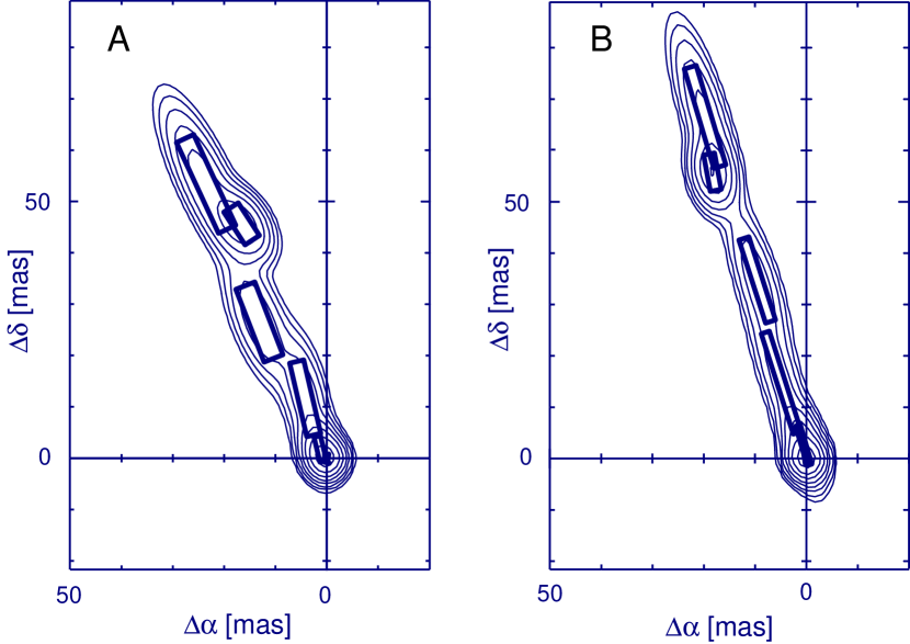
Figure 1: The surface brightness distributions for the Gaussian VLBI components (see Table 1), convolved with a circular 4-mas beam, with image $A$ on the left and $B$ on the right. Position coordinates, $\Delta\alpha$ and $\Delta\delta$, are in milliarcsec East and North on the sky, relative to the respective core components. Rectangles represent the axes and position angles of individual flux components, $A_{i}$ and $B_{i}$, where $i$ increases with distance from the core along the jet. The contours increase by factors of two from 0.55 mJy and 0.39 mJy per beam, for the A and B image maps respectively.

The VLBI image component parameter values resulting from our fit are shown in Table 1. Except for the $B_{1}$ flux density, the $B$ image positions and flux densities are derived from their $A$ image counterparts, through the image magnification matrix and its spatial derivatives. Each image component is described by a total flux density, a center position, the major axis full-width at half-maximum, the axis ratio, and the position angle of the major axis. We give component centers in relative right ascension $\Delta\alpha$ and declination $\Delta\delta$, rather than in G94’s polar coordinates. Throughout this paper our coordinates refer to epoch B1950.0  which was used for the G94 VLBI observations. The standard errors in Table 1 have been scaled to make $\bar{\chi^{2}}=1$. We do not show the parameter covariances, since these parameters were not used as direct constraints for lens models. Figure 1 shows the flux density contours of the $A$ and $B$ images as given by our model. Each image component is also represented in the figure by a rectangle whose dimensions coincide with the major and minor axes of the corresponding Gaussian. Note that the $B$ image components agree more closely with their $A$ image counterparts than is the case for G94’s VLBI component model (see Figure 3 in G94).

Table 2 presents the VLBI constraints that we use in developing lens models . These constraints include the parameter estimates, with scaled standard errors and normalized correlation coefficients, for the magnification matrix at the core and brightest jet component positions, and separately for the positions of the brightest jet components ($A_{5}$ and $B_{5}$) relative to their respective cores. Although the jet component positions in Table 2 are not independent of the magnification matrix, they do provide the most precise information on the jet structure. Thus we follow GN by including them as direct constraints to the lens models. Our results imply a relative $A\rightarrow B$ magnification of $0.74\pm 0.06$ at the core and $0.64\pm 0.04$ at the brightest jet component. The gradients of the eigenvalues along the jet direction from $A_{1}$ to $A_{5}$ (see Appendix) are $\dot{M}_{1}=(-2.6\pm 1.3)\times 10^{-3}\ {\rm mas}^{-1}$ and $\dot{M}_{2}=(4.0\pm 3.3)\times 10^{-4}\ {\rm mas}^{-1}$. These gradients differ somewhat from the values estimated by G94, of $\dot{M}_{1}=(0.5\pm 1.7)\times 10^{-3}\ {\rm mas}^{-1}$ and $\dot{M}_{2}=(2.6\pm 0.9)\times 10^{-3}\ {\rm mas}^{-1}$.

3 Other Observational Constraints

In addition to the information provided by the VLBI structures, there are a number of other observations that we use to constrain the lens models.

The separation between the two quasar images determines the mass scale of the lens model. For the $A-B$ core separation, FGS and GN adopted the value of $(-1\farcs 25271,6\farcs 04662)$ with $0\farcs 00004$ uncertainty from the original measurement of Gorenstein et al. (1984). There seems, however, to have been a slight error in FGS in the conversion from seconds to arcseconds. We use the correct value of $(-1\farcs 25254,6\farcs 04662)$. The difference is tiny and has a negligible effect on the results.

The position of the principal lens galaxy, $G1$, provides an important constraint. GN assumed the optical center of brightness of $G1$ to be at $(0\farcs 19,1\farcs 00)$ (Stockton 1980) from image B, with an uncertainty in each component of 30 mas. The lens galaxy is also detectable at radio wavelengths, and the most precise VLBI observations of the faint radio component $G^{\prime}$ yielded an estimated separation from $B$ of $(0\farcs 181,1\farcs 029)$, with a standard error of 1 mas (Gorenstein et al. 1983). Recent HST observations (B97) yield a $G1$ position of $(0\farcs 1776,1\farcs 0186)$ with $3.5$ mas errors, only about three standard deviations away from the VLBI $G^{\prime}$ position. It is not certain whether the position of the radio source or even that of the optical center coincides with the center of the lens potential within the measurement uncertainties, but as a conservative option, we have chosen to use the B97 $G1$ coordinates and errors to constrain the lens position.

In addition to the VLBI constraints G94 included two $B/A$ magnification ratios as constraints: those observed at the core and at the position of the brightest jet component. Since this jet flux ratio is incorporated in our VLBI fitting, we take only the core magnification ratio as an additional constraint. The core flux density varies over times comparable to $\Delta\tau$. To account for this, we allowed for a variable core flux ratio in the VLBI fitting, but the jet constraints alone yield a predicted magnification ratio at the core. The core magnification ratio has been independently determined to be $0.747\pm 0.015$, from a combination of optical emission line ratios with VLA and VLBI light curve analyses (see, e.g., Conner et al. 1992). If we add the directly observed core magnification ratio, we have two constraints on the same quantity and an additional degree of freedom.

Models with a smooth surface mass density for the lens produce a third image of Q0957+561, typically demagnified and near the center of the lens galaxy. No such image has been seen down to a $5\sigma$ limit of $1/30$ the flux density of image $B$ (Gorenstein et al. 1984). We follow the approach of GN in penalizing models only when their predictions exceed this $5\sigma$ limit, which GN achieve by adding to the $\chi^{2}$ a term

$$\chi^{2}_{C/B}=\left\{\begin{array}[]{ll}0&C/B<1/30\\ \frac{(C/B-1/30)^{2}}{(1/150)^{2}}&C/B>1/30\end{array}\right\},$$ (1)

where $C/B$ refers to the third image flux density ratio with respect to the $B$ image. In the SPLS model, the core radius determines the degree of central mass concentration and is the parameter most sensitive to the third-image flux limit. In the FGS model the central point mass prevents a third image from forming. Following GN, we add this constraint only in cases like the SPLS model where the third-image limit plays a role.

B97 discovered a faint arc with two bright “Knots” and a number of “Blobs”; B97 noted that the Knots, which form part of a single arc, appear to be images of each other, if the arc is indeed produced by gravitational lensing, and that two Blobs (2 and 3) are also multiple images of a background galaxy. These Blobs may differ somewhat in their peak surface brightness, but this difference may be an artifact of limited angular resolution.

We summarize the various constraints used in our model fitting in Table 3, which defines our fiducial, “full” set of constraints. Additional global constraints are given by the extended radio lobes found with the VLA (components $C$, $D$ and $E$ of Greenfield et al. 1985), which must not be multiply imaged by a lens model. We check for this constraint but do not formally include it in the $\chi^{2}$ since our models always satisfy it easily.

4 Lens Models

For modeling the gravitational lensing of Q0957+561, we consider a lens at redshift $z_{L}$ and a source at $z_{S}$, with corresponding angular diameter distances to the observer $D_{L}$ and $D_{S}$, and a lens-source distance $D_{LS}$. For a deflecting mass localized in a plane perpendicular to the line of sight, we write the lens equation (see, e.g., Schneider et al. 1992) as

$$\vec{\beta}=\vec{\theta}-\vec{\alpha}\ ,$$ (2)

where $\vec{\beta}$ is the source position, $\vec{\theta}$ is the image position, and $\vec{\alpha}$ is the deflection angle scaled by $D_{LS}/D_{S}$, all measured in the lens plane with the center of mass of the lens at the origin. We denote the mass density of the lens projected on this plane by $\Sigma$ and define a critical density $\Sigma_{c}=c^{2}D_{S}/(4\pi GD_{L}D_{LS})$. Then (in angular units) $\vec{\alpha}$ is the gradient of the two-dimensional potential $\psi$ which is determined by

$$\nabla^{2}\psi=2\frac{\Sigma}{\Sigma_{c}}\equiv 2\kappa\ .$$ (3)

If we have one lens but multiple sources at different redshifts, then to determine the corresponding $\vec{\alpha}$, a given deflection angle must be scaled by the appropriate factor of $D_{LS}/D_{S}$. Therefore, to account for the HST Blob and Knot sources in Q0957+561, whose distances are unknown, we must add additional parameters $f_{\rm blob}$ and $f_{\rm knot}$ which are the $D_{LS}/D_{S}$ ratios for each of these sources over the same ratio for the quasar.

Because of their simplicity, axisymmetric mass distributions are often used to model gravitational lenses. The Softened Power-Law Sphere (SPLS) model, defined by GN, can account for physical profiles ranging from isothermal to a point-mass, with the added possibility of a softened core. Most elliptical galaxies have central cusps in their luminosity profiles (e.g., Gebhardt et al. 1996). The possible existence of core radii in dark matter halos is unresolved, with some simulations finding a shallow inner density profile with a large scatter among halos (Kravtsov et al. 1998), while others find a density profile steeper than $1/r$ (e.g., Moore et al. 1998). The SPLS model has a spherically symmetric volume density profile,

$$\rho(r)=\rho_{0}\left(1+\frac{r^{2}}{r_{c}^{2}}\right)^{(\eta-3)/2},$$ (4)

with a corresponding projected surface density

$$\Sigma(\xi)=\Sigma_{0}\left(1+\frac{\xi^{2}}{r_{c}^{2}}\right)^{(\eta-2)/2}\ ,$$ (5)

where $\Sigma_{0}=\rho_{0}r_{C}B(1/2,1-\eta/2)$ and $B$ is the Euler beta function. The deflection law is

$$\vec{\alpha}(\vec{\theta}\,)=\left(\frac{\alpha_{E}^{2}}{\theta^{2}}\right)\left[\frac{(\theta^{2}+\theta_{c}^{2})^{\eta/2}-\theta_{c}^{\eta}}{\alpha_{E}^{\eta}}\right]\vec{\theta}\ ,$$ (6)

where $\alpha_{E}=\alpha_{0}^{2/(2-\eta)}\theta_{C}^{-\eta/(2-\eta)}$ and in radians

$$\alpha_{0}=\left(\frac{8\pi G\Sigma_{0}r_{c}^{2}}{c^{2}D\eta}\right)^{1/2}\ ,$$ (7)

with $D=D_{L}D_{S}/D_{LS}$. We note that the corresponding dimensionless surface density (i.e. convergence) is

$$\kappa(\theta)=\frac{\eta}{2}\alpha_{E}^{2-\eta}(\theta^{2}+\theta_{c}^{2})^{\frac{\eta}{2}-1}\ .$$ (8)

The parameters are thus a normalization $\alpha_{E}$, core radius $\theta_{c}$, and power-law index $\eta$.

We also use the empirical model introduced by FGS, which consists of a King profile and a central point mass. FGS adopted an analytic approximation introduced by Young et al. (1981) for the deflection law of the King profile:

$$\vec{\alpha}(\vec{\theta}\,)\ [{\rm radians}] = \left(\frac{D_{L}}{D}\right)\left(\frac{\sigma_{v}^{2}}{c^{2}}\right)\alpha_{*}(\theta)\ \hat{\theta}\ ,$$ (9)

$$\alpha_{*}(\theta) = 53.2468\,f\left(1.155\frac{\theta}{\theta_{c}}\right)-44.0415\,f\left(0.579\frac{\theta}{\theta_{c}}\right)\ ,$$

$$f(x) = \frac{\sqrt{1+x^{2}}-1}{x}\ .$$

The parameters are a velocity dispersion $\sigma_{v}$ and a core radius $\theta_{c}$. The corresponding convergence is

$$\kappa(\theta) = \left(\frac{D_{L}}{D}\right)\left(\frac{\sigma_{v}^{2}}{c^{2}}\right)\left\{\frac{30.75}{\theta_{c}}g\left(1.155\frac{\theta}{\theta_{c}}\right)-\frac{12.75}{\theta_{c}}g\left(0.579\frac{\theta}{\theta_{c}}\right)\right\}\ ,$$ (10)

$$g(x) = \frac{1}{\sqrt{1+x^{2}}}\ .$$

In order to fit the data, FGS also included a point mass of mass $M_{\rm bh}$ at the center of the galaxy, which yields

$$\vec{\alpha}(\vec{\theta}\,)=\left(\frac{\alpha_{\rm bh}^{2}}{\theta^{2}}\right)\vec{\theta}\ ,$$ (11)

where the Einstein radius is

$$\alpha_{\rm bh}=\left(\frac{4GM_{\rm bh}}{c^{2}D}\right)^{1/2}=0\farcs 91\left(\frac{M_{\rm bh}}{10^{11}\,h^{-1}\,M_{\odot}}\right)^{1/2}\ .$$ (12)

Fitted models imply this point mass is $\sim 10^{11}$ $M_{\odot}$, much larger than expected for black holes, so this term should be interpreted as correcting the King profile which by itself is not steep enough near the center of the lens. Of course, the mass of the point mass may be redistributed in any axisymmetric manner (inside the $B$ image radius) without affecting the lensing, so the FGS model is not necessarily unrealistic. This ambiguity of the FGS model with respect to the central distribution of mass in the lens galaxy $G1$ makes it difficult to utilize velocity dispersion measurements to break the $H_{0}$ degeneracy.

Since galaxies are usually not observed to be axisymmetric, elliptical mass distributions offer more general and realistic lens models. They are difficult to use, however, since the deflection angle obtained by Schramm (1990) for general elliptical models requires the evaluation of rather slow numerical integrals. To add ellipticity to the lens model while avoiding this difficulty, GN used an elliptical potential model. The imaging properties of elliptical potentials have been investigated extensively (Kovner 1987, Blandford & Kochanek 1987 and Kochanek & Blandford 1987). They become identical to elliptical densities for very small ellipticities and produce similar image configurations even for moderate ellipticity (Kassiola & Kovner 1993). However, elliptical potentials cannot represent mass distributions with ellipticities exceeding about $0.5$ because the corresponding density contours acquire the artificial feature of a dumbbell shape, and the density can also become negative in some cases (Kochanek & Blandford 1987, Kassiola & Kovner 1993, Barkana 1998). Because of this, GN restricted their model to the small ellipticity of $e=0.3$ measured for the lens galaxy light profile by Bernstein et al. (1993). However, the more recent observations by B97 found that the isophotal ellipticity increases with radius, from $0.1$ to $0.4$ . Furthermore, there is no guarantee that the dark matter has the same shape as the light profile, so it is interesting to test the ability of the lensing data to constrain the dark matter ellipticity directly.

We use the SPLS density profile with elliptical isodensity contours, a model which may be called a softened power-law elliptical mass distribution (SPEMD). We calculate the deflection angle and magnification matrix of this family of models using the fast method of Barkana (1998) which avoids the numerical integrations. We parameterize the SPEMD convergence analogously to the SPLS, as

$$\kappa(\vec{\theta}\,)=\frac{\eta}{2}\alpha_{E}^{2-\eta}\left[(x^{2}/a^{2}+y^{2}+\theta_{c}^{2})^{\frac{\eta}{2}-1}\right]\ ,$$ (13)

where we write $\vec{\theta}=(x,y)$, $a$ is the axis ratio (related to the ellipticity $e=1-a$), and we assumed a major axis along the $y$-axis. More generally the major axis is rotated at an angle $\varphi_{a}$, which we measure from North through East, consistent with Bernstein et al. (1993,1997). The SPEMD thus adds $a$ and $\varphi_{a}$ to the set of parameters of the SPLS.

We also explore an elliptical density model based on the FGS profile, keeping the point mass and adding ellipticity parameters to the King profile. As we did with the SPLS, we first take the axisymmetric convergence of the FGS model and substitute $(x^{2}/a^{2}+y^{2})$ for $r^{2}$, and then rotate the major axis by an angle $\varphi_{a}$. When made elliptical, the convergence (Equation 10) in the approximation of Young et al. (1981) yields the difference of two terms, each of which corresponds to the special case of an isothermal SPEMD. The deflection angle and magnification of such a softened isothermal elliptical mass distribution has been computed analytically in terms of complex numbers by Kassiola & Kovner (1993), so it is easy to perform lens modeling with the FGS elliptical mass distribution, or FGSE.

The lensing galaxy in 0957+561 is a massive galaxy near the center of a galaxy cluster. Following FGS, we assume that the cluster deflection varies on a scale large compared to the image separation, so we expand the cluster deflection about the center of the lens galaxy and assume it has a linear deflection law, $\alpha_{i}=M_{ij}\theta^{j}$. The traceless part of the matrix $M_{ij}$ is a shear $\gamma$ with direction $\varphi_{\gamma}$, where

$$M=\gamma\left(\begin{array}[]{cc}\cos 2\varphi_{\gamma}&-\sin 2\varphi_{\gamma}\\ -\sin 2\varphi_{\gamma}&-\cos 2\varphi_{\gamma}\end{array}\right)\ .$$ (14)

Note that GN denoted the shear angle $\phi$, and we have defined $\varphi_{\gamma}=-\phi$ for consistency with measuring the position angle of a possible corresponding cluster from North through East. The trace part is a convergence $\kappa$, which corresponds to the degeneracy identified by Falco et al. (1985): Given any lens model, if we multiply the deflection $\vec{\alpha}(\vec{\theta}\,)$ by the factor $(1-\kappa)$ and at the same time include a convergence $\kappa$ in the model, the relative image positions and magnifications remain unchanged. The time delay changes, however, by the factor $(1-\kappa)$, inducing an uncertainty in the derived $H_{0}$ unless $\kappa$ can be determined. GN note that because of this, models really only determine the scaled shear $\gamma^{\prime}=\gamma/(1-\kappa)$, and (for a given measured time delay) a scaled value of h which we denote $h^{\prime}$, where $H_{0}=100\,h\,{\rm km\,s^{-1}\,Mpc^{-1}}$ is standard notation and we also have

$$H_{0}=100\,h^{\prime}\,(1-\kappa)\,{\rm km\,s^{-1}\,Mpc^{-1}}\ .$$ (15)

In models which include external shear but no explicit convergence, the mass of the lens galaxy is also related to the physical mass by the same factor of $(1-\kappa)$. This is true for $\alpha_{E}^{2-\eta}$ of the SPLS and $\sigma_{v}^{2}$ and $M_{\rm bh}$ of the FGS model. As noted above, a direct measurement of the mass of the lens galaxy or the cluster can determine $\kappa$. Hereafter we use the symbol $\kappa$ to refer to the convergence produced by the cluster only.

As an independent attempt to determine $\kappa$, we also model the cluster as a Singular Isothermal Sphere (SIS) with a variable position, letting the fit determine the position as well as the velocity dispersion. For this model, $\rho(r)\propto 1/r^{2}$, $\Sigma(\xi)\propto 1/\xi$, and

$$\vec{\alpha}(\vec{\theta}\,)=b_{\rm cl}\hat{\theta}^{\prime}\ ,\ \ \ \ \ b_{\rm cl}=4\pi\left(\frac{\sigma_{\rm cl}}{c}\right)^{2}\frac{D_{L}}{D}=17\farcs 3\left(\frac{\sigma_{\rm cl}}{1000\,{\rm km\,s}^{-1}}\right)^{2}\ ,$$ (16)

where $\sigma_{\rm cl}$ is the velocity dispersion of the cluster and $\vec{\theta}^{\prime}=\vec{\theta}-\vec{\theta}_{\rm cl}$. The cluster parameters in this case are thus $\sigma_{\rm cl}$ and the coordinates $(x_{\rm cl},y_{\rm cl})$ of the cluster center $\vec{\theta}_{\rm cl}$ with respect to the lens galaxy position. GN considered this type of profile for the cluster but did not use it as part of their lens model. Bernstein et al. (1993) included an isothermal cluster in some of their models. Some information can be obtained from lens modeling about the cluster position, because of the influence of terms of higher order than the shear. However, fitted models imply a cluster far from the lens galaxy and the results are similar to those obtained for a cluster at an infinite distance. Therefore in the external shear model, while $h^{\prime}$ (which doesn’t include the effect of the cluster convergence) gives only an upper limit to the value of $h$, we can obtain an estimate of $h$ by assuming an SIS cluster at infinite distance, i.e. at a distance large compared to the image separation. In this case, since the external shear model determines $\gamma^{\prime}$ while an SIS cluster has $\kappa=\gamma$, we obtain an estimate for $h$ of

$$h_{\rm SIS}=h^{\prime}/(1+\gamma^{\prime})\ .$$ (17)

We can now count the number of degrees of freedom (ndof) for various models. We have 8 position constraints (core and jet $(x,y)$ positions in images $A$ and $B$, all relative to an observed lens position) and 6 magnification constraints (relative magnification matrix at the brightest jet component plus the two eigenvalues at the core). We add an independent core flux ratio constraint, and there is one more constraint for non-singular models which produce a third image. The SPLS and FGS models have 9 parameters : 3 for the lens galaxy profile , 2 for the external shear, and 4 for the two source positions. Two more parameters are added to the elliptical models, and one more when the SIS cluster is used instead of external shear. If we interpret the B97 Blob and Knot components as two additional pairs of lensed images, then each pair adds 4 position constraints and one flux ratio. Each pair also adds to the model a source position (2 parameters) and a variable source redshift, since the redshifts of these faint sources have not been measured. Thus, e.g., the ndof is 6 for the SPLS model fit only to the VLBI data and the third image flux limit, and 8 for the FGSE model fit to the VLBI data, the core flux ratio, and the HST Knots and Blobs of B97.

5 Results & Discussion

In this section we apply the lens models defined in §4 to the constraints described in §§2 and 3, and discuss the results which are summarized in Table 4. For each model, we use $\bar{\chi}^{2}$ to denote the reduced $\chi^{2}$, and estimate $95\%$ confidence bounds as in GN, from the conservative condition $\Delta\chi^{2}=4\bar{\chi}^{2}$. Confidence ranges are included for the FGSE model and all $H_{0}$ values, to illustrate the scale of our uncertainties. We also assume an Einstein-deSitter $\Omega=1$ cosmology in deriving $H_{0}$ values. The effects of this assumption are small for standard cosmologies, e.g., an open $\Omega=0.3$ universe increases the $H_{0}$ estimate by $\sim 6\%$, while a flat $\Omega_{\rm matter}=0.3$ universe with a cosmological constant yields an increase of only $\sim 4\%$. Finally, we use the Kundić et al. (1997) time delay measurement of 417$\pm$3 days, throughout.

We begin with the axisymmetric models for the lens galaxy together with the external shear model for the cluster, and fit to the full set of constraints (Table 3). The first two columns of Table 4 show the best-fit parameters for the SPLS and FGS models (for $\kappa=0$). Note that some of the parameter values using our corrected constraints differ substantially from the corresponding results of GN. However, the new constraints are very poorly fit, with $\bar{\chi}^{2}$ values over three times those of GN.

The lens galaxy is observed to be elliptical (B97), and when we add ellipticity as a parameter the lens models gain great flexibility. The $\bar{\chi}^{2}$ values are considerably lower for the elliptical SPEMD and FGSE models (see Table 4), and are comparable to the GN goodness-of-fit estimates. As a check, we tried using the SPLS profile with elliptical isopotentials as used by GN, instead of the elliptical isodensity contours of the SPEMD, and this fit gave similar parameter values to the SPEMD but with a larger $\bar{\chi}^{2}$ of 14. The $H_{0}$ estimates are very different for the FGSE and SPEMD models, but the FGSE has a much lower $\bar{\chi}^{2}$. The FGSE model also provides a closer match to the observed galaxy orientation ($\varphi_{\rm obs}\approx 40^{\circ}$, with a scatter of $\sim 10^{\circ}$, see B97). Mass and light tend to align to within $\sim 10^{\circ}$ in other lens systems, once external tides are accounted for (Keeton, Kochanek, & Falco 1998). Unfortunately, the two sources of asymmetry in both models are nearly degenerate, which tends to increase the error ranges on all parameter estimates. FGSE models with zero external shear are within our 2$\sigma$ range, implying that there is no lower limit on $\gamma^{\prime}$, and that $\phi_{\gamma}$ is undetermined. For both the FGSE and SPEMD models, the ellipticity is high, and for the FGSE model $h_{\rm SIS}$ increases steadily as $a$ decreases. If we constrain the ellipticity to equal the highest value observed for the light (i.e., axis ratio set to 0.6, see B97), we decrease $h_{\rm SIS}$ to 1.01 for the FGSE model, yielding $\bar{\chi}^{2}=8.0$. The SPEMD with $a=0.6$ yields $h_{\rm SIS}=0.626$ with $\bar{\chi}^{2}$=10.4 .

A more accurate description of the cluster contribution could remove much of the uncertainty in the models. Note that the FGSE and SPEMD models make very different $H_{0}$ predictions, with the SPEMD requiring four times as much external shear. We can model the cluster contribution by replacing the external shear with a simplified cluster mass model (see, e.g., Kochanek 1993). For example, our FGSE+CL model combines a shear-less FGSE model with a movable SIS cluster mass distribution. The overall $\bar{\chi^{2}}$ is comparable to that of the FGSE but the estimated values for some of the parameters are substantially changed. The $h$ estimate is very similar to that for the FGSE, but the uncertainty has increased from $\sim 20\%$ to $\sim 30\%$, demonstrating the sensitivity of the result to the assumed model. Figure 2 shows the appearance of the source and image planes for this model. We compare in Figure 3 the estimates from the FGSE and FGSE+CL lens models with the estimates from observations of the cluster center and velocity dispersion. Both of the observed cluster positions (Fischer et al. 1997) are offset from $G1$ in the same direction, and agree approximately with the positions from the two lens models. Note that the external shear model does not depend on whether the cluster lies to the East or West of $G1$, but the SIS cluster model breaks this degeneracy in favor of the observed direction. Still, the observational uncertainties encompass most of the models within our 2$\sigma$ contour. Likewise, the observed velocity dispersions (Fischer et al. 1997; Garrett et al. 1992; Angonin-Willaime et al. 1994) agree with the model estimates, and are too imprecise to distinguish between the models. The error estimates on cluster parameters also depend strongly on the effective $\gamma^{\prime}$, which produces large uncertainties for FGS models due to the weaker cluster contribution. Nevertheless, it is clear that more precise measurements of the cluster properties should provide significant constraints on the lens models. For example, if we assume a cluster velocity dispersion of 715 km/s and place the cluster center at the same distance ($32\farcs 2$) as the “galaxies” position, derived from number counts (see Figure 3), we obtain $h=1.05$ with $\bar{\chi}^{2}=49.3/9=5.5$. The same velocity dispersion and a distance of $22\farcs 2$, corresponding to the “weak” position from weak lensing, lowers $h$ further to 0.86 with $\bar{\chi}^{2}=82.3/9=9.1$. More precise cluster measurements may also result in $G1$ mass estimates which are more typical of a massive elliptical galaxy. For the clusters at the “galaxies” and “weak” positions, the corresponding $G1$ velocity dispersions $\sigma_{v}$ are 378 km/s and 331 km/s, respectively.

Thus far, we have assumed an SIS cluster profile, but other profiles would yield different estimates of $h$. We can explore the effect of different cluster profiles by approximating the cluster as an external shear $\gamma$ and convergence $\kappa$. Then, given $\gamma^{\prime}$ and $h^{\prime}$, there is a relation between $\gamma$ and $\kappa$ for each cluster profile and position which allows us to estimate both, and thus $h=h^{\prime}(1-\kappa)$. Figure 4 illustrates the effect on the estimate of $h$ of using different profiles for the simple, hypothetical case of $\gamma^{\prime}=0.20$ and $h^{\prime}=1.00$ . If we assume that the cluster is spherically symmetric and described by the SPLS profile, the estimate of $h$ depends on the cluster power-law index $\eta$ and on the distance to the cluster from the lens galaxy in units of the cluster core radius. If the cluster is singular, even large deviations in $\eta$ from the isothermal value of unity have a small effect on the estimated $h$. This insensitivity results from the estimates of $\kappa$ being small, so large fractional changes in $\kappa$ produce smaller fractional changes in $(1-\kappa)$. On the other hand, if $G1$ is within a few cluster core radii of the cluster center, then the SPLS profile approaches a constant density sheet (corresponding to a $1/r$ density profile in 3 dimensions); so with $\gamma^{\prime}$ fixed, $\kappa$ is driven toward 1 and $h$ decreases. The observations of Fischer et al. (1997) imply a cluster core radius of $5\pm 5\arcsec$, for an isothermal cluster. This accuracy is insufficient for use in lens modeling; the determination of the cluster’s mass distribution from weak lensing is difficult because of the insufficient number of faint background sources in the small central area of the cluster. However, a more precise determination of the cluster’s center and mass profile may allow us to distinguish between some models, and thus further reduce the model uncertainties.

As noted in §3, the center of $G1$ has been estimated from VLBI (Gorenstein et al. 1983) and HST (B97) observations; we denote these positions as $G^{\prime}$ and $G1$, respectively. If we substitute the $G^{\prime}$ position with its 1 mas standard errors for the $G1$ position in Table 3, then the parameter estimates are almost unchanged for the SPEMD and FGSE models. Of course, it is not clear how close the center of light — radio or optical — is to the mass center of the galaxy. It is correspondingly unclear what standard deviation should be used for these possible separations. Moreover, the mass distribution may not follow the shape of the light distribution, which has an ellipticity that varies with radius (B97). As an extreme case, we can assume an effectively infinite position uncertainty, by removing the lens position constraint. The resultant fit to an SPEMD model has $\bar{\chi}^{2}=57.9/7=8.3$, with $a=0.48$, $\varphi_{a}=-16\hbox{${}^{\circ}$}$, $h_{\rm SIS}=0.796$, and the estimated lens center is displaced by $(21,-78)$ mas from $G1$’s optical center. The corresponding values for the FGSE model are $\bar{\chi}^{2}=22.9/6=3.8$, with $a=0.53$, $\varphi_{a}=-1\hbox{${}^{\circ}$}$, $h_{\rm SIS}=1.01$ and the lens displaced by $(45,-44)$ mas. These large estimated lens displacements from the center of light call for a general study of how much the mass and light centers should differ in the cores of elliptical galaxies. If we allow the center of mass for $G1$ to be as far as $\sim 80$ mas away from the optical center, then the estimated $h_{\rm SIS}$ changes by $\sim 20\%$. Another indication of uncertainty in our models is that image $B$ is well inside the effective radius of $G1$ ($R_{\rm eff}\sim 4\farcs 5$, Bernstein et al. 1993), while image $A$ lies just outside this radius. Although we might expect that the galaxy mass is dominated by stars out to the distance of $B$, there may be a significant dark matter contribution at the radius of $A$, requiring a more complicated model.

Since our full set of constraints supplies a fairly large number of degrees of freedom, we can explore the robustness of the results by observing the effect of removing individual constraints. If, e.g., we use the FGSE model without including the HST Blobs (but including the Knots), we find $\bar{\chi}^{2}=9.1/6=1.5$ with $a=0.15$, $\varphi_{a}=73\hbox{${}^{\circ}$}$, and $h_{\rm SIS}=0.340$. This estimated ellipticity is much higher than that of the light distribution, which suggests that the FGSE model is not well constrained without the Blobs. By contrast, the Knots are only weak constraints due to the large errors associated with their positions and fluxes. The results are thus clearly sensitive to which constraints are included.

As another test of robustness, we used the FGSE model with the full set of constraints but we recomputed the VLBI constraints requiring the $B$ image component shapes also to agree with those of the $A$ image through the spatially-varying magnification transformation. The resulting parameter values and uncertainties are almost identical to the FGSE results in Table 4, but with $\bar{\chi}^{2}=10.0$, higher than before.

Our models also yield estimates of the distances to the HST objects. For example, the FGSE $f_{\rm blob}$ and $f_{\rm knot}$ values correspond to redshifts of $z_{\rm blob}=1.64$ and $z_{\rm knot}=3.54$ for $\Omega=1$. Assuming an open $\Omega=0.3$ universe or a flat universe with $\Omega_{\rm matter}=0.3$ increases $z_{\rm knot}$ by about 50% and 20% respectively, but for both cases $z_{\rm blob}$ increases by only a few percent. The allowed 2$\sigma$ ranges are wide, (e.g., $1.15<z_{\rm blob}<2.42$ and $1.82<z_{\rm knot}<12.2$ for $\Omega=1$) so the Blob and Knot sources could be at the same distance for any of these cosmologies. Note that all of our models predict additional fainter counterimages of the Knot source close to the observed Blob images (Figure 2). Such counterimages may have been marginally detected (Avruch et al. 1997) in the HST images. If the Knot and Blob sources are physically associated, the additional Knot images could provide more stringent lensing constraints.

Large-scale mass fluctuations along the line-of-sight to Q0957+561 can produce an additional source of uncertainty in the $H_{0}$, which will be important if the cluster is properly modeled. Barkana (1996) shows that large-scale structure affects the determination of $H_{0}$ with an uncertainty $\Delta_{1}$, but for models which are normalized to the $G1$ velocity dispersion, the velocity dispersion effectively constrains part of the effect of large-scale structure, and a smaller uncertainty $\Delta_{2}$ is left over. Given the source and lens redshifts for Q0957+561, a suite of models for the power spectrum of large-scale structure (Barkana 1996 and Figure 2 of Keeton et al. 1997) yields typical $2\sigma$ uncertainties of $\Delta_{1}=9.8\%$ and $\Delta_{2}=5.5\%$.

It is often argued that $H_{0}$ estimates from the Q0957+561 time delay are less reliable than those obtained from other lensed systems, because the cluster contribution is important. But most of the other systems for which a time delay has been measured have significant lensing contributions from a nearby group of galaxies. Although the cluster in Q0957+561 is more dominant than a smaller group would be, its mass distribution can, in principle, be directly measured. Only limited information on the cluster is presently available, but future prospects are promising for deeper weak lensing observations and for high-resolution X-ray measurements with the AXAF satellite. It may even be possible to check the cluster for dominant substructure with AXAF. Another possibility for determining indirectly the cluster contribution to lensing was suggested by Romanowsky & Kochanek (1998), who used the velocity dispersion measurement of $G1$ to estimate its mass distribution via detailed modeling of the stellar velocity distribution. Unfortunately, the result depends on the mass distribution near the center of $G1$, which is poorly determined by lens models, especially for the FGS profile which has a large point mass at the center. A possible solution is to construct a lens model which follows the light shape near the center but becomes an independent dark matter halo farther out. The present data cannot constrain the additional parameters necessary for such a lens model.

6 Conclusions

We have used improved data in the analysis of the gravitational lens system Q0957+561. We re-analyzed the VLBI data of G94 with corrected numerical procedures, and obtained new estimates for the components and spatial gradients of the relative magnification matrix between the $A$ and $B$ images. We also included new lensing constraints from recently discovered optical components (B97). The VLBI and optical constraints were used to determine more elaborate lens models than had been previously explored. In particular, we considered models with two sources of asymmetry: ellipticity in the lens galaxy and external shear from the surrounding cluster of galaxies.

Models with an axially symmetric lens are unable to fit the data, yielding $\bar{\chi}^{2}=23$ for the SPLS and $\bar{\chi}^{2}=27$ for the FGS model (all with the optical $G1$ lens position). Adding ellipticity as a model parameter leads to $\bar{\chi}^{2}=9.9$ for the SPEMD model and $\bar{\chi}^{2}=6.0$ for the FGSE model. The $H_{0}$ estimates derived from these two models differ substantially, with $h_{\rm SIS}=0.61^{+.18}_{-.16}$ and $h_{\rm SIS}=1.23^{+.22}_{-.23}$, respectively, where the uncertainties correspond to two standard deviations when an SIS cluster is used to represent the external shear. The two models can be distinguished, in principle, since they differ greatly in predicting the lens ellipticity direction and the magnitude of the cluster shear. Direct measurements of the cluster mass distribution thus have great potential.

The simple lens models that we have considered cannot be uniquely constrained by VLBI measurements alone. The HST Blobs and Knots (B97) have lines of sight that are far away from those for the $A$ and $B$ images, and could eliminate highly elliptical lens models that are permitted by the basic VLBI and core flux constraints. The discovery of more background sources in the field, or other extended radio structures (see, e.g., Avruch et al. 1997), might eventually distinguish between models, and thus narrow the allowed range of $H_{0}$. New structures may also provide enough constraints to permit the application of more complicated and realistic mass models which can account for all of the observations. A reliable measurement of $H_{0}$ may be achievable by combining the results from several such well-studied lensed systems.

7 APPENDIX

The two images $A$ and $B$, and hence their VLBI components, are related by a relative magnification mapping. Up to an irrelevant translation, we can describe the mapping from image $A$ to image $B$ by:

$$\bf{x}^{B}_{i}=\bf{M}^{BA}_{ij}\bf{x}^{A}_{j}+\frac{1}{2}\bf{\partial M}^{BA}_{ijk}\bf{x}^{A}_{j}\bf{x}^{A}_{k}\ ,$$ (18)

where repeated indices are summed. Here, $\bf{x}^{A}$ and $\bf{x}^{B}$ are the respective positions in the $A$ and $B$ images, referred to the origins at the centers of their respective cores; $\bf{M}^{BA}$ is the $2\times 2$ relative magnification matrix, evaluated at the center of $A_{1}$; and $\bf{\partial M}^{BA}$ is the tensor that represents the next order term in a Taylor series expansion (this tensor, by definition, is symmetric with respect to its last two indices). There are thus 4 independent parameters that define $\bf{M}^{BA}$ and 6 that define $\bf{\partial M}^{BA}$. The data, however, which are confined to a relatively small region, are sensitive only to the magnification derivatives along the jet direction, and weakly even to these. When we attempt estimates which include all 6 independent components of $\bf{\partial M}^{BA}$ the resultant values for most components are much higher than is physically reasonable. Thus, we remove the parameters to which our data are insensitive.

The mapping of Equation 18 describes the expansion of the relative magnification matrix $\bf{M}^{BA}(\bf{x}^{A})$ about the origin:

$$\bf{M}^{BA}_{ij}(\bf{x}^{A})\equiv\frac{\partial\bf{x}^{B}_{i}}{\partial\bf{x}^{A}_{j}}=\bf{M}^{BA}_{ij}+\bf{\partial M}^{BA}_{ijk}\bf{x}^{A}_{k}\ .$$ (19)

For such a position-dependent magnification matrix, a Gaussian representation of flux density components in the $A$ jet is no longer mapped to a corresponding Gaussian representation in the $B$ jet. In our analysis, however, we ignore the variation of $\bf{M}^{BA}$ over the extent of a component; thus we map component $A_{4}$, for example, to $B_{4}$ using a relative magnification matrix, from Equation 19, evaluated at the center of $A_{4}$. This approximation provides another reason for our treating the error estimates conservatively. Following Gorenstein et al. (1988) and G94, we decompose the matrix $\bf{M}^{BA}$ into its eigenvalues ($M_{1}$ and $M_{2}$) and the corresponding position angles of the eigenvectors ($\phi_{1}$ and $\phi_{2}$). The matrix can be represented as

$${\bf M^{BA}}=M_{1}{\bf E}(\phi_{1},\phi_{2})+M_{2}{\bf E}(\phi_{2},\phi_{1})\ ,$$ (20)

where

$$\bf{E}(\rho,\sigma)=\left[\begin{array}[]{c}\cos\rho\\ \sin\rho\end{array}\right]\cdot\left[\begin{array}[]{cc}-\sin\sigma&\cos\sigma\end{array}\right]\cdot\csc(\rho-\sigma)\ ,$$ (21)

in the notation of G94, but without rotating coordinates to align with the $A$ jet as do G94. Because of the limited sensitivity of our data, we restrict our estimation to a subset of the $\bf{\partial M}^{BA}$ parameters. We fix $\phi_{1}$ and $\phi_{2}$ to be constant along both the jet axis and the perpendicular direction, which is slightly different from the procedure of G94. Thus, we fix four $\bf{\partial M}^{BA}$ components through:

$$\bf{\partial M}^{BA}_{221} = \frac{\bf{M}^{BA}_{21}}{\bf{M}^{BA}_{12}}\bf{\partial M}^{BA}_{122}\ ,$$

$$\bf{\partial M}^{BA}_{211} = \frac{\bf{M}^{BA}_{21}}{\bf{M}^{BA}_{12}}\bf{\partial M}^{BA}_{121}\ ,$$

$$\bf{\partial M}^{BA}_{111} = \frac{\bf{M}^{BA}_{21}}{\bf{M}^{BA}_{12}}\bf{\partial M}^{BA}_{122}-\frac{\bf{M}^{BA}_{22}-\bf{M}^{BA}_{11}}{\bf{M}^{BA}_{12}}\bf{\partial M}^{BA}_{121}\ ,$$ (22)

$$\bf{\partial M}^{BA}_{222} = \bf{\partial M}^{BA}_{121}+\frac{\bf{M}^{BA}_{22}-\bf{M}^{BA}_{11}}{\bf{M}^{BA}_{12}}\bf{\partial M}^{BA}_{122}\ ,$$

leaving only two independent components of the derivative matrix.

Figure 2: Source and image planes for the FGSE+CL model. We show the source positions for the Blobs ($\bullet$), the Knots ($\Box$), and the quasar ($Q$), as well as corresponding image positions of the Blobs ($b$), the Knots ($k$), and the quasar ($A$ and $B$), all relative to the lens galaxy ($G$). The caustics (inner pair) and critical curves (outer pair) are shown for the $z=1.4$ quasar (solid lines) and the higher redshift Knot source (dashed lines). The corresponding curves for the Blob source would fall between them. The Knot source is just inside its caustic, producing the close pair of observed Knot images, as well as two faint counterimages near the two Blobs.

Figure 3: Cluster properties for the FGSE and FGSE+CL models compared to observations. The top panel shows the cluster position relative to the lens galaxy $G1$ (labeled $G$ in the Figure). The quasar image locations ($A$ and $B$) are also shown. From the FGSE model with shear we derive the direction to the cluster center (solid line) with a $2\sigma$ range (dashed lines), assuming only a spherical cluster. From the FGSE+CL model, we derive the cluster center ($\Box$) and its $2\sigma$ contour (dotted curve). Also shown are the estimated “weak” cluster center from weak lensing, and the “galaxies” position from galaxy number counts (Fischer et al. 1997). These observed positions have large uncertainties which are not shown, roughly $28\arcsec$ and $21\arcsec$ respectively, at $1\sigma$. The bottom panel compares the predicted cluster velocity dispersion to the Fischer et al. estimate from weak lensing (“weak”), and the measured dispersion (“galaxies”) for 21 probable cluster members (Garrett et al. 1992; Angonin-Willaime et al. 1994). Observed errors are again $1\sigma$ ranges. The effective velocity dispersion of the FGSE plus shear model is shown as a solid curve, with dashed 2$\sigma$ error range curves, assuming the SIS relation $\gamma=\kappa$, and the FGSE+CL best-fit and 2$\sigma$ contour are shown as above. Unlike Table 4, in this figure all $2\sigma$ errors from lens models are the formal errors of $\Delta\chi^{2}=4$ for one variable and $\Delta\chi^{2}=6.17$ for two variables.

Figure 4: Contours of constant convergence and corresponding values of $h$, shown as a function of cluster properties. The cluster is assumed to have an SPLS profile, with its $\eta$ as the $x$-axis. The $y$-axis is the distance of the cluster from the lens galaxy divided by the cluster core radius. Values of $\kappa$ are indicated at the top for each contour, with the corresponding value of $h$ for the hypothetical case of $\gamma^{\prime}=0.20$ and $h^{\prime}=1.00$.

Table 1: VLBI Component Parameters

Component	Flux	$\Delta\alpha$	$\Delta\delta$	Maj. Axis	Axis Ratio	Pos. Ang.
	(mJy)	(mas)	(mas)	(mas)		$(\hbox{${}^{\circ}$})$
$A_{1}$	$8.7\pm 1.0$	0	0	$1.6\pm 0.2$	$0.51\pm 0.15$	$-1\pm 8$
$A_{2}$	$7.6\pm 1.1$	$1.3\pm 0.1$	$1.8\pm 0.3$	$5.0\pm 0.4$	$0.26\pm 0.05$	$13\pm 3$
$A_{3}$	$3.9\pm 0.5$	$4.2\pm 0.2$	$11.7\pm 0.8$	$14.7\pm 2.1$	$0.19\pm 0.03$	$13\pm 2$
$A_{4}$	$4.7\pm 0.3$	$13.1\pm 0.2$	$26.5\pm 0.4$	$15.2\pm 1.2$	$0.26\pm 0.03$	$21\pm 2$
$A_{5}$	$9.1\pm 0.4$	$16.6\pm 0.1$	$45.6\pm 0.1$	$7.5\pm 0.3$	$0.44\pm 0.02$	$33\pm 1$
$A_{6}$	$8.8\pm 0.5$	$23.5\pm 0.3$	$53.4\pm 0.5$	$19.5\pm 1.0$	$0.19\pm 0.01$	$25\pm 1$
$B_{1}$	$7.2\pm 0.5$	0	0	$2.0\pm 0.2$	$0.37\pm 0.10$	$9\pm 3$
$B_{2}$	$5.5\pm 0.6$	$0.5\pm 0.2$	$2.6\pm 0.5$	$8.0\pm 0.8$	$0.12\pm 0.05$	$16\pm 1$
$B_{3}$	$2.8\pm 0.4$	$4.9\pm 0.4$	$14.8\pm 1.0$	$20.5\pm 3.7$	$0.08\pm 0.03$	$18\pm 2$
$B_{4}$	$2.8\pm 0.2$	$9.6\pm 0.2$	$34.8\pm 0.7$	$17.0\pm 1.8$	$0.12\pm 0.03$	$18\pm 2$
$B_{5}$	$5.8\pm 0.3$	$18.3\pm 0.1$	$55.8\pm 0.2$	$7.2\pm 0.4$	$0.30\pm 0.02$	$11\pm 1$
$B_{6}$	$4.8\pm 0.4$	$19.8\pm 0.3$	$66.5\pm 0.9$	$20.2\pm 1.5$	$0.12\pm 0.01$	$17\pm 1$

Note. — $B$ image fluxes and positions are not independently determined, they are directly related to the corresponding $A$ image values through the magnification transformation given in Table 2. We give the estimated $1\sigma$ errors on the parameters. Positions are measured relative to the respective core components. Position angles are measured in the direction North through East.

Table 2: VLBI Constraints

Quantity	Measured	correlation coefficients
		$A_{5}\Delta\alpha$	$A_{5}\Delta\delta$	$B_{5}\Delta\alpha$	$B_{5}\Delta\delta$
$A_{5}\Delta\alpha$ (mas)	$16.6\pm 0.1$	1.00
$A_{5}\Delta\delta$ (mas)	$45.6\pm 0.1$	0.26	1.00
$B_{5}\Delta\alpha$ (mas)	$18.32\pm 0.07$	–0.40	0.27	1.00
$B_{5}\Delta\delta$ (mas)	$55.8\pm 0.2$	–0.12	0.19	0.36	1.00
		$M_{1}$ at $A_{5}$	$M_{2}$ at $A_{5}$	$\phi_{1}$	$\phi_{2}$	$M_{1}$ at $A_{1}$	$M_{2}$ at $A_{1}$
$M_{1}$ at $A_{5}$	$1.15\pm 0.03$	1.00
$M_{2}$ at $A_{5}$	$-0.56\pm 0.03$	0.05	1.00
$\phi_{1}$ $(\hbox{${}^{\circ}$})$	$18.76\pm 0.04$	–0.27	0.25	1.00
$\phi_{2}$ $(\hbox{${}^{\circ}$})$	$107\pm 7$	–0.34	–0.74	–0.16	1.00
$M_{1}$ at $A_{1}$	$1.27\pm 0.03$	–0.95	–0.02	0.20	0.16	1.00
$M_{2}$ at $A_{1}$	$-0.58\pm 0.04$	–0.06	0.985	0.31	–0.70	0.09	1.00

Note. — Results of simultaneous fitting to the $A$ and $B$ images, where the positions and fluxes of the $B$ jet components are fixed by the $A$ jet components and the $A\rightarrow B$ mapping, but the shapes are not. We give the estimated $1\sigma$ errors on the parameters, the normalized position correlation coefficients, and the magnification correlation coefficients. The component positions for $A_{5}$ and $B_{5}$, from Table 1, are included as separate constraints as they provide the most precise information on the jet structure.

Table 3: “Full set” of constraints

Constraint	Value(s)	${\rm N_{const}}$	Comments
Magnification matrix	See Table 2	6	from fit to VLBI data
$A_{5}$ position	See Table 2	2	from fit to VLBI data
$B_{5}$ position	See Table 2	2	from fit to VLBI data
$A_{1}$ core position	$(-1\farcs 25254,6\farcs 04662)\pm 0\farcs 00004$	2	corrected from FGS
$B_{1}/A_{1}$ magnif	$0.747\pm 0.015$	1	Conner et al. 1992
$C/B_{1}$ magnif	$<1/30$	$1^{*}$	as in GN; ∗non-FGS only
lens center	$(0\farcs 1776,1\farcs 0186)\pm 0\farcs 0035$	2	G1, from HST, B97
Blob East pos	$(1\farcs 72,0\farcs 98)\pm 0\farcs 05$	2	Blob 2, B97
Blob West pos	$(-2\farcs 70,4\farcs 48)\pm 0\farcs 05$	2	Blob 3, B97
Blobs magnif ratio	$-1.3\pm 0.14$ mag	1	Blobs 2/3 flux, B97
Knot East pos	$(0\farcs 13,-1\farcs 53)\pm 0\farcs 05$	2	Knot 1, B97
Knot West pos	$(-0\farcs 29,-1\farcs 41)\pm 0\farcs 05$	2	Knot 2, B97
Knot magnif ratio	$-0.3\pm 0.7$ mag	1	Knots 1/2 flux, B97

Note. — All positions are offsets ($\Delta\alpha$,$\Delta\delta$) from the $B_{1}$ core position.

Table 4: Best fit model results

Parameter	SPLS	FGS	SPEMD	FGSE	FGSE+CL
Lensing galaxy:
$x_{\rm lens}-x_{G1}$	40.4 mas	16.4 mas	6.3 mas	$4.4^{+17}_{-16}$ mas	2.5 mas
$y_{\rm lens}-y_{G1}$	0.0 mas	2.5 mas	–1.7 mas	$-0.2^{+17}_{-17}$ mas	–0.2 mas
$\theta_{c}$	$0\farcs 00$	$2\farcs 58$	$0\farcs 17$	$1\farcs 59^{+1.6}_{-0.2}$	$1\farcs 39$
$\alpha_{E}$ or $\sigma_{v}$	$2\farcs 45$	378 km/s	$3\farcs 98$	$447^{+350}_{-54}$ km/s	404 km/s
$\eta$ or $M_{\rm bh}$	1.16	107 $\times 10^{9}$M⊙	1.01	92.5${}^{+14}_{-26}$ $\times 10^{9}$M⊙	69.9 $\times 10^{9}$M⊙
$a$	$\cdots$	$\cdots$	0.469	$0.445^{+.15}_{-.32}$	0.505
$\varphi_{a}$	$\cdots$	$\cdots$	$123\fdg 8$	$67\fdg 3^{+18}_{-19}$	$61\fdg 9$
Cluster contribution:
$\gamma^{\prime}$	0.258	0.209	0.364	$0.083^{+.10}_{-\mbox{---}}$	$\cdots$
$\varphi_{\gamma}$	$66\fdg 4$	$65\fdg 0$	$51\fdg 9$	$63\fdg 4\pm\mbox{---}$	$\cdots$
$\sigma_{\rm cl}$	$\cdots$	$\cdots$	$\cdots$	$\cdots$	439 km/s
$x_{\rm cl}-x_{G1}$	$\cdots$	$\cdots$	$\cdots$	$\cdots$	$13\farcs 7$
$y_{\rm cl}-y_{G1}$	$\cdots$	$\cdots$	$\cdots$	$\cdots$	$6\farcs 9$
HST sources:
$f_{\rm blob}$	1.06	1.02	1.03	$1.05^{+.10}_{-.13}$	1.05
$f_{\rm knot}$	1.08	0.95	1.09	$1.22^{+.12}_{-.14}$	1.12
General:
ndof	11	10	9	8	7
$\bar{\chi}^{2}$	23	27	9.9	6.0	5.9
$h$ or $(h_{\rm SIS})$	$(0.619^{+.06}_{-.03})$	$(0.657^{+.11}_{-.28}$)	$(0.629^{+.16}_{-.18})$	$(1.23^{+.22}_{-.23})$	$1.13^{+.32}_{-.27}$

Note. — Using the full constraint set in Table 3. Errors, where given, are defined by $\Delta\chi^{2}=4\bar{\chi}^{2}$.

References

- (1) Avruch, I. M., Cohen, A. S., Lehár, J., Conner, S. R., Haarsma, D. B., & Burke, B. F. 1997, ApJ, 488, L121
- (2) Angonin-Willaime, M. C., Soucail, G., & Vanderriest, C. 1994, A& A, 291, 411
- (3) Barkana, R. 1996, ApJ, 468, 17
- (4) Barkana, R. 1997, ApJ, 489, 21
- (5) Barkana, R. 1998, ApJ, 502, 531
- (6) Bernstein, G., Fischer, P., Tyson, J. A., & Rhee, G. 1997, ApJ, 483, L79 (B97)
- (7) Bernstein, G. M., Tyson, J. A., & Kochanek, C. S. 1993, AJ, 105, 816
- (8) Biggs, A. D., Browne, I. W. A., Helbig, P., Koopmans, L. V. E., Wilkinson, P. N., & Perley, R. A. 1999, to appear in MNRAS
- (9) Blandford, R. D., & Kochanek, C. S. 1987, ApJ, 321, 658
- (10) Blandford, R. D., & Narayan, R. 1992, ARA&A, 30, 311
- (11) Campbell, R. M., Lehár, J., Corey, B. E., Shapiro, I. I., & Falco, E. E. 1995, AJ, 110, 2566
- (12) Cawthorne, T. V. 1991, in Beams and Jets in Astrophysics, ed. Hughes, P. A. (Cambridge Univ. Press: Cambridge)
- (13) Chartas, G., Chuss, D., Forman, W., Jones, C., & Shapiro, I. 1998, ApJ, 504, 661
- (14) Conner, S. R., Lehár, J., & Burke, B. F. 1992, ApJ, 387, L61
- (15) Falco, E. E., Gorenstein, M.V., & Shapiro, I. I. 1985, ApJ, 289, L1
- (16) Falco, E. E., Shapiro, I. I., Moustakas, L. A., & Davis, M. 1997, ApJ, 484, 70
- (17) Falco, E. E., Gorenstein, M. V., & Shapiro, I. I. 1991, ApJ, 372, 364
- (18) Fassnacht, C. D., Pearson, T. J., Blandford, R. D., & Readhead, A. C. S. 1997, in Radio Emission from Galactic and Extragalactic Compact Sources, IAU Colloquium No. 164
- (19) Fischer, P., Bernstein, G., Rhee, G., & Tyson, J. A. 1997, A&A, 113, 521
- (20) Florentin-Nielsen, R. 1984, A&A, 138, L19
- (21) Garrett, M. A., Calder, R. J., Porcas, R. W., King, L. J., Walsh, D., & Wilkinson, P. N. 1994, MNRAS, 270, 457 (G94)
- (22) Garrett, M. A., Walsh, D., & Carswell, R. F. 1992, MNRAS, 254, 27p
- (23) Gebhardt et al. 1996, AJ, 112, 105
- (24) Gorenstein, M. V., Cohen, N. L., Shapiro, I. I. Rogers, A. E. E., Bonometti, R. J., Falco, E. E., Bartel, N, & Marcaide, J. M. 1988, ApJ, 334, 42
- (25) Gorenstein, M. V., Shapiro, I. I., Rogers, A. E. E., Cohen, N. L., Corey, B. E., Porcas, R. W., Falco, E. E., Bonometti, R. J., Preston, R. A., Rius, A., & Whitney, A. R. 1984, ApJ, 287, 538
- (26) Gorenstein, M. V., Shapiro, I. I., Corey, B. E., Falco, E. E., Marcaide, J. M., Cohen, N. L., Rogers, A. E. E., Whitney, A. R. 1984, Porcas, R. W., Preston, R. A., 1983, Science, 219, 54
- (27) Greenfield, P. D., Roberts, D. H., & Burke, B. F. 1985, ApJ, 293, 370
- (28) Grogin, N. A., & Narayan, R. 1996, ApJ, 464, 92; erratum, ApJ, 473, 570 (GN)
- (29) Haarsma, D. B., Hewitt, J. N., Lehár, J., & Burke, B. F. 1998, accepted by ApJ, astro-ph/9807115
- (30) Impey, C. D., Falco, E. E., Kochanek, C. S., Lehár, J., Mcleod, B. A., Rix, H.-W., Peng, C. Y., & Keeton, C. R. 1998, ApJ, 509, 551
- (31) Kassiola, A., & Kovner, I. 1993, ApJ, 417, 450
- (32) Keel, W. C. 1982, ApJ, 255, 20
- (33) Keeton, C. R., Kochanek, C. S., & Falco, E. E. 1998, ApJ, 509, 561
- (34) Keeton, C. R., Kochanek, C. S., & Seljak, U. 1997, ApJ, 482, 604
- (35) Kochanek, C. S. 1991, ApJ, 382, 58
- (36) Kochanek, C. S. 1993, ApJ, 419, 12
- (37) Kochanek, C. S., & Blandford, R. D. 1987, ApJ, 321, 676
- (38) Kovner, I. 1987, Nature, 325, 507
- (39) Kravtsov, A. V., Klypin, A. A., Bullock, J. S., & Primack, J. R. 1998, ApJ, 502, 48
- (40) Kundić, T., Turner, E. L., Colley, W. N., Gott, J. R., Rhoads, J. E., Wang, Y., Bergeron, L. E., Gloria, K. A., Long, D. C., Malhorta, S., & Wambsganss, J. 1997, ApJ, 482, 75
- (41) Lehár, J., Hewitt, J. N., Roberts, D. H., & Burke, B. F. 1992, ApJ, 384, 453
- (42) Lloyd, C. 1981, Nature, 294, 727
- (43) Mao, S., & Schneider, P. 1998, MNRAS, 295, 587
- (44) Moore, B., Governato, F., Quinn, T., Stadel, J., & Lake, G. 1998, ApJ, 499, L5
- (45) Pelt, J., Hoff, W., Kayser, R., Refsdal, S., & Schramm, T. 1994, A&A, 286, 775
- (46) Pelt, J., Kayser, R., Refsdal, S., & Schramm, T. 1996, A&A, 305, 97
- (47) Porcas, R. W., Booth, R. S., Browne, I. W. A., Walsh, D., & Wilkinson, P. N. 1981, Nature, 289, 758
- (48) Press, W. H., Rybicki, G. B., & Hewitt, J. N. 1992a, ApJ, 385, 404
- (49) Press, W. H., Rybicki, G. B., & Hewitt, J. N. 1992b, ApJ, 385, 416
- (50) Refsdal, S. 1964, MNRAS, 128, 307
- (51) Refsdal, S. 1966, MNRAS, 132, 101
- (52) Rhee, G. 1991, Nature, 350, 211
- (53) Romanowsky, A. J., & Kochanek, C. S. 1998, astro-ph/9805080
- (54) Schechter, P. L., et al. 1997, ApJ, 475, L85
- (55) Schild, R. E., & Cholfin, B. 1986, ApJ, 300, 209
- (56) Schild, R., & Thomson, D. J. 1995, AJ, 109, 1970
- (57) Schneider, P., Ehlers, J., & Falco, E.E. 1992, Gravitational Lenses (New York: Springer)
- (58) Schramm, T. 1990, A&A, 231, 19
- (59) Stockton, A. 1980, ApJ, 242, L141
- (60) Tonry, J. L., Franx, M., 1998, to appear in ApJ, astro-ph/9809064
- (61) Vanderriest, C., Schneider, J., Herpe, G., Chevreton, M., Moles, M., & Wlérick, G. 1989, A&A, 215, 1
- (62) Walsh, D., Carswell, R. F., & Weymann, R. J. 1979, Nature, 279, 381
- (63) Wisotzki, L., Wucknitz, O., Lopez, S., & Sørensen, A. N. 1998, A&A, 339, 73
- (64) Young, P., Gunn, J. E., Kristian, J., Oke, J. B., & Westphal, J. A. 1980, ApJ, 241, 507
- (65) Young, P., Gunn, J. E., Kristian, J., Oke, J. B., & Westphal, J. A. 1981, ApJ, 244, 736