THE SUNYAEV-ZEL’DOVICH EFFECT

Abstract

The Sunyaev-Zel’dovich effect causes a change in the apparent brightness of the Cosmic Microwave Background Radiation towards a cluster of galaxies or any other reservoir of hot plasma. Measurements of the effect provide distinctly different information about cluster properties than X-ray imaging data, while combining X-ray and Sunyaev-Zel’dovich effect data leads to new insights into the structures of cluster atmospheres. The effect is redshift-independent, and so provides a unique probe of the structure of the Universe on the largest scales. The present review discusses the theory of the Sunyaev-Zel’dovich effect and collects published results for many clusters, presents the overall conclusions that may be drawn from the detections so far, and discusses the prospects for future research on the Sunyaev-Zel’dovich effects.

1 Astrophysical Context

Compton scattering is one of the major physical processes that couples matter and radiation. Its importance is often stressed in highly relativistic environments where large energy transfers occur: for example, in the synchrotron self-Compton process that may be responsible for much of the X-radiation from active galactic nuclei (e.g., Fabian et al. 1986). However, the Compton process also has observable consequences in low-energy environments, where small energy transfers occur. The Sunyaev-Zel’dovich effect, which arises from the scattering of electrons in clusters of galaxies on the cosmic microwave background radiation field, is perhaps the most important astrophysical example. The effect provides a cosmological probe, it has been used to measure the properties of gas in clusters of galaxies, and it has been discussed as a means of measuring the motions of clusters of galaxies and hence studying the evolution of structure in the Universe.

The purpose of this review is to provide a comprehensive introduction to the Sunyaev-Zel’dovich effect. I aim to provide both a theoretical treatment that can be followed by non-specialists, and an introduction to the observation of the effect with a critical review of data in the literature. The latter is more difficult today than it would have been five years ago because of the rapid increase in the number of papers on the Sunyaev-Zel’dovich effect, and the improvement in the quality of the results that are being gained.

1.1 The Cosmic Microwave Background Radiation

The cosmic microwave background radiation (CMBR) is the dominant radiation field in the Universe, and one of the most powerful cosmological tools that has yet been found. 25 years after its discovery by Penzias & Wilson (1965) much is now known about the properties of the radiation (see the recent review by Partridge 1995), and a vigorous community studies the CMBR to extract all the cosmological and astrophysical data that it carries.

Within a few years of the discovery of the CMBR, it was established the radiation field is close to isotropic, with a spectrum characterized by a single temperature, ${T_{\rm rad}}\approx 2.7\ \rm K$. The specific intensity of the radiation is therefore close to

$$I_{\nu}={2\,h\,\nu^{3}\over c^{2}}\,\left(e^{h\nu/k_{\rm B}{T_{\rm rad}}}-1\right)^{-1}$$ (1)

which corresponds to a peak brightness $I_{\rm max}\sim 3.7\times 10^{-18}\ \rm W\,m^{-2}\,Hz^{-1}\,sr^{-1}$ at $\nu_{\rm max}\sim 160\ \rm GHz$, a photon density $n_{\gamma}\sim 4\times 10^{8}\ \rm photons\,m^{-3}$, and an energy density $u_{\gamma}\sim 4\times 10^{-14}\ \rm J\,m^{-3}$, which can also be expressed as a mass density $\rho_{\gamma}\sim 5\times 10^{-31}\ \rm kg\,m^{-3}$, much less than the critical density

$$\rho_{\rm crit} = {3H_{0}^{2}\over{8\pi G}}$$ (2)

$$= 1.88\times 10^{-26}\,h_{100}^{2}\quad\rm kg\,m^{-3}$$

required to close the Universe. In these equations, $h$ is Planck’s constant, $c$ is the speed of light, $\nu$ is the frequency, $k_{\rm B}$ is the Boltzmann constant, $G$ is the gravitational constant, and $h_{100}=H_{0}/100\ \rm km\,s^{-1}\,Mpc^{-1}$ is a dimensionless measure of the value of the Hubble constant, $H_{0}$. Recent estimates give $0.5\lesssim h_{100}\lesssim 0.8$ (e.g., Sandage et al. 1996; Falco et al. 1997; Sandage & Tammann 1997; Freedman, Madore & Kennicutt 1997).

Although specific small parts of the sky (stars, radio sources, and so on) are brighter than the CMBR, overall the CMBR constitutes the major electromagnetic radiation field in the Universe and contributes about 60 per cent of the relativistic energy density (the other 40 per cent being provided by the neutrinos, assumed to be massless here). The integrated brightness of the sky in the CMBR is not small, and a comparison with a bright radio source may be useful. Cygnus A is one of the brightest extragalactic radio sources at low frequencies. A comparison of the relative brightness of Cygnus A and the CMBR, as observed by a telescope with a 1 square degree beam, is shown in Figure 1. It can be seen that the CMBR easily dominates over a wide range of frequencies above 10 GHz. It is not signal strength that makes measuring the intensity of the CMBR difficult, but rather the problem of making absolute measurements, since the CMBR is present in all directions with almost equal intensity.

1.2 Thermal history of the Universe and the CMBR

The origins of the CMBR lie in an early hot phase of the expansion of the Universe, where the details of its generation are erased by the close coupling of radiation and matter. Later energy releases, interactions with matter at different temperatures, and other effects can modify the spectrum and brightness distribution of the CMBR. Cosmological data on the gross properties of the Universe are contained in the integrated properties of the CMBR, such as the spectrum and the large-scale brightness structure. Detailed information about the properties and formation of present-day objects, such as clusters of galaxies, is encoded in the small-scale structures in the brightness.

A critical stage in the development of the CMBR occurs when the expansion of the Universe causes the temperature to drop to about $3000\ \rm K$. At earlier times (higher redshifts), matter and radiation were in good thermal contact because of the abundance of free electrons. But at this stage the number of free electrons drops rapidly as matter becomes neutral, and the radiation and matter become thermally decoupled, so that the temperatures of the photon and matter fluids evolve almost independently. We can distinguish three events that occur at almost the same time: the non-relativistic and relativistic (photon plus neutrino) mass densities are equal at redshift

$$z_{\rm eq}=2.5\times 10^{4}\,\Omega_{0}h_{100}^{2},$$ (3)

most electrons have become bound to ions at the redshift of recombination,

$$z_{\rm rec}=1.4\times 10^{3}\,(\Omega_{\rm B}h_{100}^{2})^{0.02},$$ (4)

and the interaction length of photons and electrons exceeds the scale of the Universe at the redshift of decoupling

$$z_{\rm dec}=1.1\times 10^{3}\,(\Omega_{0}/\Omega_{\rm B})^{0.02}$$ (5)

(approximate forms taken from Kolb & Turner 1990). In these relations, $\Omega_{0}$ is the present-day mass density of the Universe, and $\Omega_{\rm B}$ is the present-day baryon density, both in units of the critical density, $\rho_{\rm crit}$ (equation 2). The redshifts of recombination and decoupling are similar, and neither phenomenon is sharply-defined, so that there was a moderately broad redshift range from $1500$ to $1000$ (about $1.6\times 10^{5}(\Omega_{0}h_{100}^{2})^{-1/2}$ years after the Big Bang) when the Universe was becoming neutral, matter-dominated, and transparent to radiation. At some time about then, most of the photons that are now in the cosmic background radiation were scattered by electrons for the last time, and we often refer to a sphere of last scattering or redshift of last scattering at this epoch.

One of the important changes that occurred during this period, because of the change in the interactions of photons and electrons, was that the length scale on which gravitational collapse can occur dropped dramatically, so that fluctuations in the mass density that were stabilized by the radiation field before recombination became unstable after recombination, and were able to collapse (slowly — the expansion of the Universe causes the collapse of gravitationally bound objects to be power-law rather than exponential in time: Landau & Lifshitz 1962; see descriptions in Kolb & Turner 1990). Matter over-densities and under-densities present at recombination, and which later became the large-scale objects that we see in the present-day Universe, such as clusters of galaxies, caused fluctuations in the intensity of the radiation field through their gravitational perturbations (the Sachs-Wolfe effect; Sachs & Wolfe 1967), through thermodynamic fluctuations in the density of radiation coupled to the matter, and through Doppler shifts due to motions of the surface of last scattering. Recent reviews of the introduction of primordial structure in the CMBR by objects near recombination are given by Bond (1995) and White, Scott & Silk (1994).

1.3 COBE and the CMBR

Much of the best data on the large-scale structural and spectral properties of the CMBR was gathered by the Cosmic Background Explorer (COBE) satellite (Boggess et al. 1992). The accuracy with which the spectrum of the radiation matches a black body with temperature ${T_{\rm rad}}=2.728\pm 0.002\ {\rm K}$ (Fixsen et al. 1996) demonstrates that the Universe has been through a dense, hot, phase and provides strong limits on non-thermalized cosmological energy transfers to the radiation field (Wright et al. 1994). The previously-known dipolar term in the CMBR anisotropy was better measured — Fixsen et al. find an amplitude $3.372\pm 0.004$ mK. This dipole is interpreted as arising mostly from our peculiar motion relative to the sphere of last scattering, and this motion was presumably induced by local masses (within 100 Mpc or so). Our implied velocity is $371\pm 1\ {\rm km\,s^{-1}}$ towards galactic coordinates $l=264^{\circ}\hbox to0.0pt{\hss.}14\pm 0^{\circ}\hbox to0.0pt{\hss.}15$, $b=48^{\circ}\hbox to0.0pt{\hss.}26\pm 0^{\circ}\hbox to0.0pt{\hss.}15$ . It is interesting to note that this dipolar anisotropy shows an annual modulation from the motion of the Earth around the Sun (Kogut et al. 1994) and a spectral shape consistent with the first derivative of a black body spectrum (Fixsen et al. 1994), as expected. This modulation was used to check the calibration of the COBE data.

After the uniform (monopole) and dipolar parts of the structure of the CMBR are removed, there remain significant significant correlated signals in the angular power spectrum. These signals correspond to an an rms scatter of $35\pm 2\ {\rm\mu K}$ on the $7^{\circ}$ scale of the COBE DMR beam (Banday et al. 1997), much larger than any likely residual systematic errors (Bennett et al. 1996), and hold information about the radiation fluctuations at the sphere of last scattering which are caused by density and temperature fluctuations associated with the formation of massive structures (such as clusters of galaxies). Their amplitude can be described by a multipole expansion of the brightness temperature variations

$$\Delta T(\theta,\phi)=\sum_{lm}\,a_{lm}\,Y_{lm}(\theta,\phi)$$ (6)

with power spectrum

$$P_{l}=|a_{l}|^{2}={1\over 2l+1}\,\sum_{m}\,|a_{lm}|^{2}.$$ (7)

It is usually assumed that the $a_{lm}$ obey Gaussian statistics, as measured by a set of observers distributed over the Universe. The ensemble of values of $a_{lm}$ for each $(l,m)$ then has a zero mean with a standard deviation dependent on $l$ only and a phase that is uniformly distributed over $0$ to $2\pi$. In that case, the temperature field is completely specified by the two-point correlation function

$$C(\theta)=\langle T({\bf n}_{\rm a})\,T({\bf n}_{\rm b})\rangle$$ (8)

where the average is over all observers, and $\cos\theta={\bf n}_{\rm a}{\bf.}{\bf n}_{\rm b}$ is the angle between the directions ${\bf n}_{\rm a}$ and ${\bf n}_{\rm b}$. For a Gaussian random field,

$$C(\theta)={1\over 4\pi}\sum_{l}\,(2l+1)\,C_{l}\,P_{l}(\cos\theta)$$ (9)

where $C_{l}=\langle|a_{lm}|^{2}\rangle$. For such a spectrum and correlation function, it can be shown that a power-law initial density fluctuation spectrum, $P(k)\propto k^{n}$ will produce a spectrum with

$$C_{l}=C_{2}\,{\Gamma\left(l+{1\over 2}(n-1)\right)\,\Gamma\left({1\over 2}(9-n)\right)\over\Gamma\left(l+{1\over 2}(5-n)\right)\,\Gamma\left({1\over 2}(3+n)\right)}$$ (10)

if $n<3$, $l\geq 2$, and the Sachs-Wolfe effect dominates the primordial fluctuations (Bond & Efstathiou 1987). In this case, the character of the fluctuations is usually described by the best-fitting index $n$ and

$$Q_{\rm rms-PS}=\left({5\over 4\pi}C_{2}\right)^{1/2}$$ (11)

which is the mean rms temperature fluctuation expected in the quadrupole component of the anisotropy averaged over all cosmic observers and obtained by fitting the correlation function by a flat spectrum of fluctuations.

For the 4-year COBE DMR data, the best-fitting power spectrum of the fluctuations has $n=1.2\pm 0.3$ and $Q_{\rm rms-PS}=15^{+4}_{-3}\ {\rm\mu K}$ (Gorski et al. 1996), although different analyses of the data by the COBE team give slightly different errors and central values (Wright et al. 1996; Hinshaw et al. 1996). These values are consistent with the scale-invariant Harrison-Zel’dovich spectrum (Harrison 1970; Zel’dovich 1972; Peebles & Yu 1970), with $n=1$ ($P(k)\propto k$), and hence with the usual picture of random fluctuations growing to form galaxies and clusters of galaxies following a phase of inflation (Starobinsky 1980; Guth 1981; Bardeen, Steinhardt & Turner 1983).

1.4 Clusters of galaxies and the CMBR

If the CMBR were undisturbed from the epoch of decoupling, where it picks up these “primordial” anisotropies from structure formation, to the present, then all perturbations in the background could be interpreted in terms of early processes in the Universe. If there are strong interactions between the epoch of decoupling and the present, then all the perturbations associated with the formation of structure might have been overwritten by later effects (e.g., from a smoothly re-ionized and dense intergalactic medium; Tegmark, Silk & Blanchard 1994).

The true appearance of the CMBR lies between these two extremes. Even away from obvious local structures (such as stars and radio sources) there are a number of structures in the Universe that can affect the propagation of radiation. For example, gravitational lenses redistribute radiation from the epoch of recombination. Were this radiation to be isotropic, then there would be no effect from a static lens. However, a lens would affect the detailed pattern of anisotropies that are imposed on the CMBR at recombination, and detailed studies of these anisotropies should take that effect into account, especially on the smallest angular scales (e.g., Blanchard & Schneider 1987; Sasaki 1989; Watanabe & Tomita 1991). Even an isotropic radiation field may pick up anisotropies from lenses, if those lenses are not static. Examples of such effects have been discussed by Rees & Sciama (1968), Dyer (1976), Nottale (1984), Gott (1985), Gurvits & Mitrofanov (1986), and Birkinshaw (1989).

These metric (Rees-Sciama) perturbations of the isotropy of the background radiation tend to be small, of order the gravitational lensing angle implied by the mass ($\Delta\theta\sim{4GM/Rc^{2}}$, where $M$ is the object’s mass and $R$ its size or the impact parameter) multiplied by a dimensionless measure of the extent to which the lens is non-static. For example, the fractional intensity change is of order $\Delta\theta\,(v/c)$ for a lens moving across the line of sight with velocity $v$. For even the largest masses (of clusters of galaxies), for which $\Delta\theta\sim 1$ arcmin), and the largest likely velocities ($\sim 10^{3}\ {\rm km\,s^{-1}}$), the fractional intensity change $\Delta I_{\nu}/I_{\nu}\lesssim 10^{-6}$. It is interesting that redshift and angular effects introduced by spatial and temporal metric variations of a perturbing mass are closely related (Pyne & Birkinshaw 1993), and can be fitted into the same formalism as the Sachs-Wolfe effect (Sachs & Wolfe 1967), which is the dominant source of anisotropy in the microwave background radiation on the angular scale of the COBE experiments.

The most likely sources for metric perturbations of the CMBR are clusters of galaxies, which are the most massive well-differentiated structures in the Universe. However the structures introduced by metric effects associated with clusters of galaxies will be very difficult to see because of the presence of the Sunyaev-Zel’dovich effects, which are also introduced by clusters, but which are far more intense.

The basic physics of the Sunyaev-Zel’dovich effect is simple. Clusters of galaxies have masses that often exceed $3\times 10^{14}\ {M_{\odot}}$, with effective gravitational radii, $R_{\rm eff}$, of order Mpc. Any gas in hydrostatic equilibrium within a cluster’s gravitational potential well must have electron temperature ${T_{\rm e}}$ given by

$${k_{\rm B}}{T_{\rm e}} \approx {GM{m_{\rm p}}\over 2R_{\rm eff}}$$ (12)

$$\approx 7\,(M/3\times 10^{14}\,{M_{\odot}})\,(R_{\rm eff}/{\rm Mpc})^{-1}\qquad{\rm keV}.$$

At this temperature, thermal emission from the gas appears in the X-ray part of the spectrum, and is composed of thermal bremsstrahlung and line radiation.

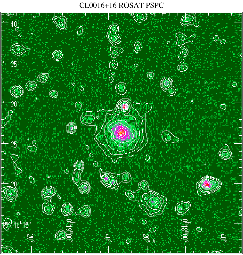
Figure 2: The central region of the ROSAT PSPC X-ray image containing the distant cluster CL 0016+16 ($z=0.5455$), showing the extended X-rays produced by the thermal emission of gas in approximate hydrostatic equilibrium in the cluster’s potential well. The coordinates are in epoch J2000. The data, extracted from PI bins 0.4–2.4 keV, have been background subtracted, exposure corrected, and adaptively smoothed. The effective spatial resolution of this image is $\sim$30^′′ (half-power diameter). Contour levels start at a value of $1.8\times 10^{-4}$ counts s^-1 arcmin^-2 (75 per cent of the average background level) and increase by multiplicative factors of 1.94. The bright X-ray source immediately to the north of the cluster is an AGN, QSO 0015+162, at a redshift $z=0.554$. Note the extended source to the southwest which is a poor cluster, RX J0018.3+1618, at a redshift $z=0.5506$ (Hughes, Birkinshaw & Huchra 1995).

About a quarter of the mass of clusters of galaxies is in the form of distributed gas (e.g., White & Fabian 1995; Elbaz, Arnaud & Böhringer 1995; David et al. 1995; Dell’Antonio, Geller & Fabricant 1995). The density of the gas is sufficiently high that clusters of galaxies are luminous X-ray sources (e.g., Figure 2; see the reviews of Forman & Jones 1982; Sarazin 1988), with the bulk of the X-rays being produced as bremsstrahlung rather than line radiation. Electrons in the intracluster gas are not only scattered by ions, but can themselves scatter photons of the CMBR: for these low-energy scatterings the cross-section is the Thomson scattering cross-section, $\sigma_{\rm T}$, so that the scattering optical depth $\tau_{\rm e}\approx n_{\rm e}\,\sigma_{\rm T}\,R_{\rm eff}\sim 10^{-2}$. In any one scattering the frequency of the photon will be shifted slightly, and up-scattering is more likely. On average a scattering produces a slight mean change of photon energy $(\Delta\nu/\nu)\approx({k_{\rm B}}{T_{\rm e}}/m_{\rm e}c^{2})\sim 10^{-2}$. The overall change in brightness of the microwave background radiation from inverse Compton (Thomson) scattering is therefore about 1 part in $10^{4}$, a signal which is about ten times larger than the cosmological signal in the microwave background radiation detected by COBE.

The primordial and Sunyaev-Zel’dovich effects are both detectable, and can be distinguished by their different spatial distributions. Sunyaev-Zel’dovich effects are localized: they are seen towards clusters of galaxies, which are large-scale structures visible to redshifts $>0.5$ in the optical and X-ray bands. Furthermore, the amplitude of the signal should be related to other observable properties of the clusters. Primordial structures in the CMBR are non-localized: they are not associated with structures seen at other wavebands, and are distributed at random over the entire sky, with almost constant correlation amplitude in different patches of sky.

It is on the Sunyaev-Zel’dovich effects that the present review concentrates. Although the original discussion and detection of the effects were driven by the question of whether cluster X-ray emission arose from the hot gas in cluster potential wells or from non-thermal electrons interacting with magnetic fields or the cosmic background radiation (Sunyaev & Zel’dovich 1972), more recently the effects have been studied for the information that they can provide on cluster structures, on the motions of clusters of galaxies relative to the Hubble flow, and on the Hubble flow itself (and the cosmological constants that characterize it). The last few years have seen many new detections of Sunyaev-Zel’dovich effects from clusters with strong X-ray emission — and the special peculiarity of the Sunyaev-Zel’dovich effects, that they are redshift-independent, and therefore almost as easy to observe at high as at low redshift, has been illustrated by detecting clusters as distant as CL 0016+16, at $z=0.5455$, or at even higher redshift.

2 Radiation basics

Although the CMBR is close to being an isotropic and thermal radiation background with simple spectral and angular distributions, it is useful to recall the formalism needed to deal with a general radiation field, since the details of the small perturbations have great physical significance. The notation used here is similar to that of Shu (1991), which may be consulted for more detailed descriptions of the quantities employed.

The state of a radiation field can be described by distribution functions $f_{\alpha}({\bf r},{\bf p},t)$, such that the number of photons in real space volume $d^{3}r$ about $\bf r$ and momentum space volume $d^{3}p$ about $\bf p$ at time $t$ with polarization $\alpha$ ($=1$ or $2$) is $f_{\alpha}\,d^{3}r\,d^{3}p$. This distribution function is related to the photon occupation number in polarization state $\alpha$, $n_{\alpha}({\bf r},{\bf p},t)$, by

$$f_{\alpha}({\bf r},{\bf p},t)=h^{-3}\,n_{\alpha}({\bf r},{\bf p},t)$$ (13)

and to the specific intensity in the radiation, $I_{\nu}({\bf\hat{k}},{\bf r},t)$, by

$$I_{\nu}({\bf\hat{k}},{\bf r},t)=\sum_{\alpha=1}^{2}\,\left({h^{4}\,\nu^{3}\over c^{2}}\right)\,f_{\alpha}({\bf r},{\bf p},t)$$ (14)

where ${\bf\hat{k}}$ is a unit vector in the direction of the radiation wavevector, $\nu$ is the photon frequency, and $h$ and $c$ are Planck’s constant and the speed of light. The meaning of the specific intensity is that the energy crossing area element $\bf dS$ in time $dt$ from within solid angle $d\Omega$ about $\bf\hat{k}$ and with frequency in the range $\nu$ to $\nu+d\nu$ is $I_{\nu}\,({\bf\hat{k}.dS})\,d\Omega\,d\nu\,dt$.

If the occupation number is of Planck form

$$n_{\alpha}=\left(e^{h\nu/{k_{\rm B}}{T_{\rm rad}}}-1\right)^{-1}\quad\rm for\ \alpha=1,2$$ (15)

then the radiation field has the form of (1). The number density of photons in the Universe is then

$$n_{\gamma} = \sum_{\alpha}\int f_{\alpha}({\bf p})\,d^{3}p$$ (16)

$$= 16\,\pi\,\zeta(3)\,\left({{k_{\rm B}}{T_{\rm rad}}\over hc}\right)^{3}$$

$$= (4.12\pm 0.01)\times 10^{8}\quad\rm photons\,m^{-3}\qquad if\ {T_{\rm rad}}=2.728\pm 0.002\ \rm K$$

from which can be calculated the baryon to photon number ratio, $\eta={n_{\rm B}/n_{\gamma}}=2.7\times 10^{-8}\Omega_{\rm B}h_{100}^{2}$. In (16) $\zeta(x)$ is the Riemann zeta function ($\zeta(3)\approx 1.202$) and the value of ${T_{\rm rad}}$ is taken from a recent analysis of COBE data on the CMBR spectrum (Fixsen et al. 1996).

Similarly, the energy density of the radiation field is

$$u_{\gamma} = \sum_{\alpha}\int h\nu\,f_{\alpha}({\bf p})\,d^{3}p$$ (17)

$$= {8\,\pi^{5}\,h\,c\over 15}\,\left({{k_{\rm B}}{T_{\rm rad}}\over h\,c}\right)^{4}$$

$$= (4.19\pm 0.01)\times 10^{-14}\quad\rm J\,m^{-3}\qquad if\ {T_{\rm rad}}=2.728\pm 0.002\ \rm K.$$

It is apparent that the errors on $u_{\gamma}$ and $n_{\gamma}$ in (16) and (17) are so small as to have no significant astrophysical impact, and may safely be dropped.

It is common for the specific intensity of a radiation field to be described by radio-astronomers in units of brightness temperature, $T_{\rm RJ}$. This is defined as the temperature of a thermal radiation field which in the Rayleigh-Jeans limit of low frequency would have the same brightness as the radiation that is being described. In the limit of low frequency (1) reduces to $I_{\nu}=2{k_{\rm B}}{T_{\rm rad}}\nu^{2}/c^{2}$, so that

$$T_{\rm RJ}(\nu)={c^{2}I_{\nu}\over 2{k_{\rm B}}\nu^{2}}\quad.$$ (18)

Thus the brightness temperature of a thermal spectrum as described by (1) is frequency-dependent, with a peak value equal to the radiation temperature at low frequencies, and tending to zero in the Wien tail.

In the presence of absorption, emission and scattering processes, and in a flat spacetime, $I_{\nu}$ obeys a transport equation

$${1\over c}\,{\partial I_{\nu}\over\partial t}+{\bf\hat{k}}.{\bf\nabla}I_{\nu}=j_{\nu}-\alpha_{\nu,\rm abs}I_{\nu}-\alpha_{\nu,\rm sca}I_{\nu}+\alpha_{\nu,\rm sca}\int\phi_{\nu}({\bf\hat{k}},{\bf\hat{k}^{\prime}})\,I_{\nu}({\bf k^{\prime}})d\Omega^{\prime}$$ (19)

where $j_{\nu}$ is the emissivity along the path (the energy emitted per unit time per unit frequency per unit volume per unit solid angle), $\alpha_{\nu,\rm abs}$ is the absorption coefficient (the fractional loss of intensity of the radiation per unit length of propagation because of absorption by material in the beam), $\alpha_{\nu,\rm sca}$ is the scattering coefficient (the fractional loss of intensity of the radiation per unit length of propagation because of scattering by material in the beam), and $\phi_{\nu}({\bf\hat{k}},{\bf\hat{k}^{\prime}})$ is the scattering redistribution function — the probability of a scattering from direction $\bf\hat{k}^{\prime}$ to $\bf\hat{k}$. The absorption coefficient is regarded as containing both true absorption and simulated emission. While this is important in astrophysical masers, where $\alpha_{\nu,\rm abs}$ is negative, this subtlety will not affect the discussions in the present review. An important property of $I_{\nu}$ that follows from its definition (or equation 19) is that it is conserved in flat spacetimes in the absence of radiation sources or absorbers.

The specific intensity of a radiation field may be changed in several ways. One is to make the photon distribution function anisotropic, for example by the Doppler effect due to the peculiar motion of the Earth relative to the sphere of last scattering, which causes the radiation temperature becomes angle-dependent

$$T^{\prime}_{\rm rad}(\theta)={{T_{\rm rad}}\over\gamma\left(1-{v\over c}\cos\theta\right)},$$ (20)

but otherwise leaves the form of (15) unchanged. $\gamma=\left(1-{v^{2}\over c^{2}}\right)^{-1/2}$ and $\theta$ is the angle between the line of sight and the observer’s velocity vector (Peebles & Wilkinson 1968). The specific intensity may also be changed by redistributing photons to different directions and frequencies (e.g., by scattering processes), or by absorbing or emitting radiation (e.g., by thermal bremsstrahlung). The choice of whether to describe these effects in the photon distribution function, or in the specific intensity, is made for reasons of convenience. Although the statistical mechanics of photon scattering is often related to the occupation numbers, $n_{\alpha}$, most astrophysical work is done in the context of the specific intensity, $I_{\nu}$.

3 Inverse-Compton Scattering

The theoretical foundation of the Sunyaev-Zel’dovich effect was laid in the early 1970s (Sunyaev & Zel’dovich 1970), but is based on earlier work on the interactions of photons and free electrons (Kompaneets 1956; Dreicer 1964; Weymann 1965). Excellent recent reviews of the physics of the Sunyaev-Zel’dovich effect have been given by Bernstein & Dodelson (1990) and Rephaeli (1995b), while discussions of the more general problem of comptonization of a radiation field by passage through an ionized gas have been given by Blumenthal & Gould (1970), Sunyaev & Zel’dovich (1980a), Pozdnyakov, Sobol’ & Sunyaev (1983), and Nagirner & Poutanen (1994). Comptonization is also an essential ingredient in the discussion of the X-ray and gamma-ray emission of active galactic nuclei (see, for example, Zbyszewska & Zdziarski 1991; Zdziarski et al. 1993; Skibo et al. 1995). The present section relies heavily on this work, and on the material on inverse-Compton scatterings in Rybicki & Lightman (1980), and the papers by Wright (1979) and Taylor & Wright (1989).

3.1 Single photon-electron scattering

When a photon is scattered by an electron, the energy and direction of motion of both the photon and the electron are usually altered. The change in properties of the photon is described by the usual Compton scattering formula

$$\epsilon^{\prime}={\epsilon\over 1+{\epsilon\over m_{\rm e}c^{2}}\,(1-\cos\phi_{12})}$$ (21)

where the electron is assumed to be at rest before the interaction, $\epsilon$ and $\epsilon^{\prime}$ are the photon energies before and after the interaction, and $\phi_{12}$ is the angle by which the photon in deflected in the encounter (see Fig. 3).

For low-energy photons and mildly relativistic or non-relativistic electrons, $\epsilon\ll m_{\rm e}c^{2}$ and the scattering is almost elastic ($\epsilon^{\prime}=\epsilon$). This limit is appropriate for the scatterings in clusters of galaxies that cause the Sunyaev-Zel’dovich effect, and causes a considerable simplification in the physics. Although the scatterings are usually still referred to as inverse-Compton processes, they might better be described as Thomson scatterings in this limit.

Scatterings of this type will also cause Sunyaev-Zel’dovich effects from the relativistic plasma of radio galaxies. The lobes of radio galaxies emit strong synchrotron radiation, and must contain electrons with Lorentz factors $\gamma_{\rm e}\gtrsim 10^{8}$. In the rest frames of such electrons the microwave background radiation appears to have a peak at photon energies $\sim 0.1m_{\rm e}c^{2}$, and the assumption of elastic scattering will be inappropriate. Little theoretical work has been done on the spectrum of the scattered radiation in this limit, but see Section 5.

In this thermal scattering limit, the interaction cross-section for a microwave background photon with an electron need not be described using the Klein-Nishina formula,

$${d\sigma\over d\Omega}={r_{\rm e}^{2}\over 2}\,\left({\epsilon^{\prime}\over\epsilon}\right)^{2}\left({\epsilon\over\epsilon^{\prime}}+{\epsilon^{\prime}\over\epsilon}-\sin^{2}\phi_{12}\right)$$ (22)

but rather the classical Thomson cross-section formula which results in the limit $\epsilon^{\prime}\rightarrow\epsilon$. Then if the geometry of the collision process in the electron rest frame is as shown in Fig. 3, the probability of a scattering with angle $\theta$ is

$$p(\theta)\,d\theta = p(\mu)\,d\mu$$ (23)

$$= \left(2\gamma^{4}(1-\beta\mu)^{3}\right)^{-1}\,d\mu$$

where the electron velocity $v_{\rm e}=\beta c$, and $\mu=\cos\theta$. The probability of a scattering to angle $\theta^{\prime}$ is

$$\phi(\mu^{\prime};\mu)d\mu^{\prime}={3\over 8}\left(1+\mu^{2}{\mu^{\prime}}^{2}+{1\over 2}(1-\mu^{2})(1-{\mu^{\prime}}^{2})\right)\,d\mu^{\prime}$$ (24)

(Chandrasekhar 1950; Wright 1979), and the change of photon direction causes the scattered photon to appear at frequency

$$\nu^{\prime\prime}=\nu\,(1+\beta\mu^{\prime})\,(1-\beta\mu)^{-1}$$ (25)

with $\mu^{\prime}=\cos\theta^{\prime}$.

It is conventional (Wright 1979; Sunyaev 1980; Rephaeli 1995b) to express the resulting scattering in terms of the logarithmic frequency shift caused by a scattering, $s$ (Sunyaev uses $u$ for a related quantity),

$$s=\log(\nu^{\prime\prime}/\nu)$$ (26)

when the probability that a single scattering of the photon causes a frequency shift $s$ from an electron with speed $\beta c$ is

$$P(s;\beta)\,ds=\int p(\mu)\,d\mu\,\phi(\mu^{\prime};\mu)\,\left({d\mu^{\prime}\over ds}\right)\,ds.$$ (27)

Using (23–25), this becomes

$$P(s;\beta)={3\over 16\gamma^{4}\beta}\,\int_{\mu_{1}}^{\mu_{2}}\,(1+\beta\mu^{\prime})\,\left(1+\mu^{2}{\mu^{\prime}}^{2}+{1\over 2}(1-\mu^{2})(1-{\mu^{\prime}}^{2})\right)(1-\beta\mu)^{-3}\,d\mu$$ (28)

where $\mu^{\prime}$ can be expressed in terms of $\mu$ and $s$ as

$$\mu^{\prime}={e^{s}(1-\beta\mu)-1\over\beta}$$ (29)

(from equations 25 and 26), and the integral is performed only over real angles, so that

$$\mu_{1} = \cases{-1&$s\leq 0$\cr{1-e^{-s}(1+\beta)\over\beta}&$s\geq 0$\cr}$$ (30)

$$\mu_{2} = \cases{{1-e^{-s}(1-\beta)\over\beta}&$s\leq 0$\cr 1&$s\geq 0$\cr}$$ (31)

in (28). The integration can be done easily, and Fig. 4 shows the resulting function for several values of $\beta$. The increasing asymmetry of $P(s;\beta)$ as $\beta$ increases is caused by relativistic beaming, and the width of the function to zero intensity in $s$,

$$\Delta s_{0}=2\log\left({1+\beta\over 1-\beta}\right),$$ (32)

increases because increasing $\beta$ causes the frequency shift related to a given photon angular deflection to increase.

3.2 Scattering of photons by an electron population

The distribution of photon frequency shifts caused by scattering by a population of electrons is calculated from $P(s;\beta)$ by averaging over the electron $\beta$ distribution. Thus for photons that have been scattered once, the probability distribution of $s$, $P_{1}(s)$, is given by

$$P_{1}(s)=\int_{\beta_{\rm lim}}^{1}\,p_{\rm e}(\beta)\,d\beta\,P(s;\beta)$$ (33)

where $\beta_{\rm lim}$ is the minimum value of $\beta$ capable of causing a frequency shift $s$,

$$\beta_{\rm lim}={e^{|s|}-1\over e^{|s|}+1}.$$ (34)

The limitations of equation (33) are evident from the assumptions made to derive equation (28). That is, the electron distribution $p_{\rm e}(\beta)$ must not extend to sufficiently large Lorentz factors, $\gamma$, that the assumptions of elastic scattering with the Thomson scattering cross-section are violated. For photons of the microwave background radiation these assumptions are amply satisfied provided that $\gamma\lesssim 2\times 10^{9}$. In clusters of galaxies the typical electron temperatures may be as much as 15 keV ($1.8\times 10^{8}\ {\rm K}$), but the corresponding Lorentz factors are still small, so that we may ignore relativistic corrections to the scattering cross-section.

If the electron velocities are assumed to follow a relativistic Maxwellian distribution,

$$p_{\rm e}(\beta)\,d\beta={\gamma^{5}\,\beta^{2}\,\exp\left(-{\gamma\over\Theta}\right)\,d\beta\over\Theta\,K_{2}({1\over\Theta})},$$ (35)

where $\Theta$ is the dimensionless electron temperature

$$\Theta=\left({k_{\rm B}\,T_{\rm e}\over m_{\rm e}\,c^{2}}\right)$$ (36)

and $K_{2}(z)$ is a modified Bessel function of the second kind and second order, then the resulting distribution of photon frequency shift factors can be calculated by a numerical integration of equation (33).

The result of performing this calculation for $k_{\rm B}T_{\rm e}=5.1$ and 15.3 keV is shown in Fig. 5, where it is compared with the result given by Sunyaev (1980). It can be seen that the distribution of scattered photon frequencies is significantly asymmetric, with a stronger upscattering ($s>1$) tail than a downscattering tail. This is the origin of the mean frequency increase caused by scatterings. As the temperature of the electron distribution increases, this upscattering tail increases in strength and extent. Sunyaev’s (1980) distribution function tends to have a stronger tail at large values of $s$ and a larger amplitude near $s=0$ than does the form derived using (33).

It is also of interest to calculate the form of $P_{1}(s)$ for a power-law distribution of electron energies in some range of Lorentz factors $\gamma_{1}$ to $\gamma_{2}$

$$p_{\rm e}(\gamma)d\gamma=\cases{A\,\gamma^{-\alpha}\,d\gamma&$\gamma_{1}\leq\gamma\leq\gamma_{2}$\cr 0&otherwise\cr}$$ (37)

with normalizing constant

$$A=\cases{\log\gamma_{2}-\log\gamma_{1}&$\alpha=1$\cr(1-\alpha)\,\left(\gamma_{2}^{1-\alpha}-\gamma_{1}^{1-\alpha}\right)^{-1}&$\alpha\neq 1$\cr}$$ (38)

since such a population, which might be found in a radio galaxy lobe, can also produce a Sunyaev-Zel’dovich effect. Synchrotron emission from radio galaxies has a range of spectral indices, but values of $\alpha\approx 2.5$ are common. Thus Fig. 6 shows the result of a calculation for an electron population with $\alpha=2.5$. As might be expected, the upscattering tail is much more prominent in Fig. 6 than in Fig. 5, since there are more electrons with $\gamma\gg 1$ in distribution (37) than in distribution (35) for the values of $\Theta$ and $\alpha$ chosen.

3.3 Effect on spectrum of radiation

Finally it is necessary to use the result for the frequency shift in a single scattering to calculate the form of the scattered spectrum of the CMBR. If every photon in the incident spectrum,

$$I_{0}(\nu)={2\,h\,\nu^{3}\over c^{2}}\,\left(e^{h\nu/k_{\rm B}{T_{\rm rad}}}-1\right)^{-1},$$ (39)

is scattered once, then the resulting spectrum is given by

$${I(\nu)\over\nu}=\int_{0}^{\infty}d\nu_{0}\,P_{1}(\nu,\nu_{0})\,{I_{0}(\nu_{0})\over\nu_{0}}$$ (40)

where $P_{1}(\nu,\nu_{0})$ is the probability that a scattering occurs from frequency $\nu_{0}$ to $\nu$, and $I(\nu)/h\nu$ is the spectrum in photon number terms. Since $P_{1}(\nu,\nu_{0})=P_{1}(s)/\nu$, where $P_{1}(s)$ is the frequency shift function in (33), this can be rewritten as a convolution in $s=\ln(\nu/\nu_{0})$,

$$I(\nu)=\int\limits_{-\infty}^{\infty}P_{1}(s)\,I_{0}(\nu_{0})\,ds\quad.$$ (41)

The change in the radiation spectrum at frequency $\nu$ is then

$$\Delta I(\nu) \equiv I(\nu)-I_{0}(\nu)$$ (42)

$$= {2h\over c^{2}}\,\int\limits_{-\infty}^{\infty}P_{1}(s)\,ds\,\left({\nu_{0}^{3}\over e^{h\nu_{0}/{k_{\rm B}}{T_{\rm rad}}}-1}-{\nu^{3}\over e^{h\nu/{k_{\rm B}}{T_{\rm rad}}}-1}\right)$$

where the normalization of $P_{1}(s)$ has allowed the (trivial) integral over $I_{0}(\nu)$ to be included in (42) to give a form that is convenient for numerical calculation.

The integrations in (41) or (42) are performed using the $P_{1}(s)$ function appropriate for the spectrum of the scattering electrons. The results are shown in Fig. 7 and 8 for two temperatures of the electron gas and for the power-law electron distribution. In these figures, $x=h\nu/{k_{\rm B}}{T_{\rm rad}}$ is a dimensionless frequency. The functions $\Delta I(x)$ show broadly similar features for thermal or non-thermal electron distributions: a decrease in intensity at low frequency (where the mean upward shift of the photon frequencies caused by scattering causes the Rayleigh-Jeans part of the spectrum to shift to higher frequency, and hence to show an intensity decrease: see Fig. 1) and an increase in intensity in the Wien part of the spectrum. The detailed shapes of the spectra differ because of the different shapes of the scattering functions $P_{1}(s)$ (Figs. 5 and 6).

More generally, a photon entering the electron distribution may be scattered 0, 1, 2, or more times by encounters with the electrons. If the optical depth to scattering through the electron cloud is $\tau_{\rm e}$, then the probability that a photon penetrates the cloud unscattered is $e^{-\tau_{\rm e}}$, the probability that it is once scattered is $\tau_{\rm e}e^{-\tau_{\rm e}}$, and in general the probability of N scatterings is

$$p_{\rm N}={\tau_{\rm e}^{N}e^{-\tau_{\rm e}}\over N!}$$ (43)

and the full frequency redistribution function from scattering is

$$P(s)=e^{-\tau_{\rm e}}\left(\delta(s)+\tau_{\rm e}\,P_{1}(s)+{1\over 2!}\tau_{\rm e}^{2}P_{2}(s)+\ldots\right).$$ (44)

The redistribution function $P_{\rm n}(s)$ after $n$ scatterings is given by a repeated convolution

$$P_{\rm 2}(s) = \int dt_{1}P_{1}(t_{1})P_{1}(s-t_{1})$$

$$P_{\rm 3}(s) = \int dt_{1}dt_{2}P_{1}(t_{1})P_{1}(t_{2})P_{1}(s-t_{1}-t_{2})$$ (45)

$$\vdots$$

but as pointed out by Taylor & Wright (1989), the expression for $P(s)$ can be written in much simpler form using Fourier transforms, with $P(s)$ obtained by the back transform

$$P(s)={1\over\sqrt{2\pi}}\,\int_{-\infty}^{\infty}\tilde{P}(k)\,e^{iks}\,ds$$ (46)

of

$$\tilde{P}(k)=e^{-\tau_{\rm e}(\tilde{P}_{1}(k)-1)}$$ (47)

where the Fourier transform of $P_{1}(s)$ is

$$\tilde{P}_{1}(k)={1\over\sqrt{2\pi}}\,\int_{-\infty}^{\infty}P_{1}(s)\,e^{-iks}\,ds\quad.$$ (48)

The generalization of (41) for an arbitrary optical depth is then

$$I(\nu)=\int\limits_{-\infty}^{\infty}P(s)\,I_{0}(\nu_{0})\,ds$$ (49)

but this full formalism will rarely be of interest, since in most situations the electron scattering medium is optically thin, with $\tau_{\rm e}\ll 1$, so that the approximation

$$P(s)=(1-\tau_{\rm e})\,\delta(s)+\tau_{\rm e}\,P_{1}(s)$$ (50)

will be sufficient (but see Molnar & Birkinshaw 1998b). The resulting intensity change has the form shown in Fig. 7 or 8, but with an amplitude reduced by a factor $\tau_{\rm e}$. This is given explicitly as

$$\Delta I(\nu)={2h\over c^{2}}\,\tau_{\rm e}\,\int\limits_{-\infty}^{\infty}P_{1}(s)\,ds\,\left({\nu_{0}^{3}\over e^{h\nu_{0}/{k_{\rm B}}{T_{\rm rad}}}-1}-{\nu^{3}\over e^{h\nu/{k_{\rm B}}{T_{\rm rad}}}-1}\right).$$ (51)

and this form of $\Delta I(\nu)$ will be used extensively later. One important result is already clear from (51): the intensity change caused by the Sunyaev-Zel’dovich effect is redshift-independent, depending only on intrinsic properties of the scattering medium (through the $\tau_{\rm e}$ factor and $P_{1}(s)$), and the Sunyaev-Zel’dovich effect is therefore a remarkably robust indicator of gas properties at a wide range of redshifts.

3.4 The Kompaneets approximation

The calculations that led to equation (51) are accurate to the appropriate order in photon frequency and electron energy for our purposes, and take account of the relativistic kinematics and statistics of the scattering process. In the non-relativistic limit the scattering process simplifies substantially, and may be described by the Kompaneets (1956) equation

$${\partial n\over\partial y}={1\over x_{\rm e}^{2}}\,{\partial\over\partial x_{\rm e}}\,x_{\rm e}^{4}\,\left({\partial n\over\partial x_{\rm e}}+n+n^{2}\right)$$ (52)

which describes the change in the occupation number, $n({\nu})$ by a diffusion process. In (52), $x_{\rm e}={h\nu/{k_{\rm B}}{T_{\rm e}}}$, which should not be confused with $x={h\nu/{k_{\rm B}}{T_{\rm rad}}}$ used previously, and

$$y={{k_{\rm B}}{T_{\rm e}}\over m_{\rm e}c^{2}}\,{c\,t\over\lambda_{\rm e}}$$ (53)

is a dimensionless measure of time spent in the electron distribution. $\lambda_{\rm e}$ is the “Compton range”, or the scattering mean free path, $(n_{\rm e}\sigma_{\rm T})^{-1}$. For a radiation field passing though an electron cloud, $y$, which is usually known as the Comptonization parameter, can be rewritten in the more usual form

$$y=\int\,n_{\rm e}\,\sigma_{\rm T}\,dl\,{{k_{\rm B}}{T_{\rm e}}\over m_{\rm e}c^{2}}\quad.$$ (54)

Note that a time- (or $y$-) independent solution of (52) is given when the electrons and photons are in thermal equilibrium, so that $n=(e^{x_{\rm e}}-1)^{-1}$, as expected, and that the more general Bose-Einstein distributions $n=(e^{x_{\rm e}+\alpha}-1)^{-1}$ are also solutions. A derivation of equation (52) from the Boltzmann equation is given by Bernstein & Dodelson (1990).

In the limit of small $x_{\rm e}$, which is certainly appropriate for the CMBR and hot electrons, ${\partial n\over\partial x_{\rm e}}\gg n$, $n^{2}$, and (52) becomes

$${\partial n\over\partial y}={1\over x_{\rm e}^{2}}\,{\partial\over\partial x_{\rm e}}\,x_{\rm e}^{4}\,{\partial n\over\partial x_{\rm e}}.$$ (55)

The homogeneity of the right hand side of this equation allows us to replace $x_{\rm e}$ by $x$, and a change of variables from $x,y$ to $\xi,y$, where $\xi=3y+\ln x_{\rm e}$, reduces (55) to the canonical form of the diffusion equation,

$$\left({\partial n\over\partial y}\right)={\partial^{2}n\over\partial\xi^{2}}.$$ (56)

In the format of equation (49), this indicates that the solution of the Kompaneets equation can be written

$$I(\nu)=\int\limits_{-\infty}^{\infty}P_{\rm K}(s)\,I_{0}(\nu_{0})\,ds$$ (57)

where the Kompaneets scattering kernel is of Gaussian form

$$P_{\rm K}(s)={1\over\sqrt{4\pi y}}\,\exp\left(-{(s+3y)^{2}\over 4y}\right)$$ (58)

(Sunyaev 1980; Bernstein & Dodelson 1990). The difference between the scattering kernels (33) and (58) is small but significant for the mildly relativistic electrons that are important in most cases, and can become large where the electron distribution becomes more relativistic (compare the solid and dashed lines in Fig. 5). These shape changes lead to spectral differences in the predicted $\Delta I(\nu)$, which for thermal electrons can be characterized by the changing positions of the minimum, zero, and maximum of the spectrum of the Sunyaev-Zel’dovich effect with changing electron temperature. This is illustrated in Fig. 9 for a range of temperatures that is of most interest for the clusters of galaxies (Section 4).

Most work on the Sunyaev-Zel’dovich effect has used the Kompaneets equation, and implicitly the Kompaneets scattering kernel, rather than the more precise relativistic kernel (44) advocated by Rephaeli (1995a). The two kernels are the same at small ${T_{\rm e}}$, as expected since the Kompaneets equation is correct in the low-energy limit. At low optical depth and low temperatures, where the Comptonization parameter $y$ is small, and for an incident photon spectrum of the form of equation (15), the approximation ${\partial n\over\partial y}={\Delta n\over y}$ may be used in (55) to obtain a simple form for the spectral change caused by scattering

$$\Delta n=x\,y\,{e^{x}\over(e^{x}-1)^{2}}\,\left(x\,\coth(x/2)-4\right)$$ (59)

with a corresponding $\Delta I(x)=x^{3}\Delta n(x)I_{0}$, where $I_{0}={2h\over c^{2}}\left({{k_{\rm B}}{T_{\rm rad}}\over h}\right)^{3}$ again. This result can also be obtained directly from the integral (57) for $I(x)$ in the limit of small $y$. Fig. 7 compares the Kompaneets approximation for $\Delta I(x)$ with the full relativistic results.

There are three principal simplifications gained by using (59), rather than the relativistic results.

1. The spectrum of the effect is given by a simple analytical function (59).

2. The location of the spectral maxima, minima, and zeros are independent of ${T_{\rm e}}$ in the Kompaneets approximation, but vary with ${T_{\rm e}}$ in the relativistic expressions. To first order in $\Theta$, which is adequate for temperatures ${k_{\rm B}}{T_{\rm e}}<20$ keV ($\Theta<0.04$),

   $$x_{\rm min} = 2.26$$

   $$x_{\rm zero} = 3.83\,(1+1.13\Theta)$$ (60)

   $$x_{\rm max} = 6.51\,(1+2.15\Theta)$$

   as seen in Fig. 9. Earlier approximations for $x_{\rm zero}(\Theta)$ are given by Fabbri (1981) and Rephaeli (1995a).

3. The amplitude of the intensity (or brightness temperature) change depends only on $y$ ($\propto{T_{\rm e}}\tau_{\rm e}$) in the Kompaneets approximation, but in the relativistic expression the amplitude is proportional to $\tau_{\rm e}$ (for small $\tau_{\rm e}$) and also depends on a complicated function of ${T_{\rm e}}$.

It is possible to improve on the Kompaneets result (59) by working to higher order in $\Theta$ from (51) or the Boltzmann equation. The resulting expressions for $\Delta n$ or $\Delta I$ are usually written as a series in increasing powers of $\Theta$ (Challinor & Lasenby 1998; Itoh, Kohyama & Nozawa 1998; Stebbins 1998). Taken to four or five terms these series provide a useful analytical expression for the Sunyaev-Zel’dovich effect for hot clusters for a wide range of $x$. However, the expressions cannot be used blindly since they are asymptotic approximations, and are still of poor accuracy for some $(x,\Theta)$ values. The approximations also rely on the assumptions that the cluster is optically thin and that the electron distribution function is that of a single-temperature gas (35). Both assumptions are questionable when precise results (to better than 1 per cent) are needed, and so the utility of the idealized multi-term expressions is limited. For the most precise work, especially work on the kinematic Sunyaev-Zel’dovich effect (Section 6), the relativistic expressions with suitable forms for the distribution functions, and proper treatment of the cluster optical depth, must be used if accurate spectra for the effect, and hence estimates for the cluster velocities, are to be obtained (Molnar & Birkinshaw 1998b).

4 The thermal Sunyaev-Zel’dovich effect

The results in Section 3 indicate that passage of radiation through an electron population with significant energy content will produce a distortion of the radiation’s spectrum. In the present section the question of the effect of thermal electrons on the CMBR is addressed in terms of the three likely sites for such a distortion to occur:

1. the atmospheres of clusters of galaxies

2. the ionized content of the Universe as a whole, and

3. ionized gas close to us.

4.1 The Sunyaev-Zel’dovich effect from clusters of galaxies

By far the commonest references to the Sunyaev-Zel’dovich effect in the literature are to the effect that the atmosphere of a cluster of galaxies has on the CMBR. Cluster atmospheres are usually detected through their X-ray emission, as in the example shown in Fig. 2, although the existence of such gas can also be inferred from its effects on radio source morphologies (e.g., Burns & Balonek 1982) — ‘disturbed’ lobe shapes and head-tail sources being typical indicators of the presence of cluster gas.

If a cluster atmosphere contains gas with electron concentration $n_{\rm e}({\bf r})$, then the scattering optical depth, Comptonization parameter, and X-ray spectral surface brightness along a particular line of sight are

$$\tau_{\rm e} = \int n_{\rm e}({\bf r})\,\sigma_{\rm T}\,dl$$ (61)

$$y = \int n_{\rm e}({\bf r})\,\sigma_{\rm T}\,{{k_{\rm B}}{T_{\rm e}}({\bf r})\over m_{\rm e}c^{2}}\,dl$$ (62)

$$b_{\rm X}(E) = {1\over 4\pi(1+z)^{3}}\,\int n_{\rm e}({\bf r})^{2}\,\Lambda(E,T_{\rm e})\,dl$$ (63)

where $z$ is the redshift of the cluster, and $\Lambda$ is the spectral emissivity of the gas at observed X-ray energy $E$ or into some bandpass centered on energy $E$ (including both line and continuum processes). The factor of $4\pi$ in the expression for $b_{\rm X}$ arises from the assumption that this emissivity is isotropic, while the $(1+z)^{3}$ factor takes account of the cosmological transformations of spectral surface brightness and energy.

By far the most detailed information on the structures of cluster atmospheres is obtained from X-ray astronomy satellites, such as ROSAT and ASCA. Even though these satellites also provide some information about the spectrum of $b_{\rm X}$ (and hence an emission-weighted measure of the average gas temperature along the line of sight) there is no unique inversion of (63) to $n_{\rm e}({\bf r})$ and $T_{\rm e}({\bf r})$. Thus it is not possible to predict accurately the distribution of $y$ on the sky, and hence the shape of the Sunyaev-Zel’dovich effect (which we will, in the current section, take to be close to the shape of $y$, although Sec. 3.3 indicates that an accurate prediction of the Sunyaev-Zel’dovich effect requires a more complicated calculation which includes both the electron scattering optical depth and the gas temperature).

In many cases it is then convenient to introduce a parameterized model for the properties of the scattering gas in the cluster, and to fit the the values of these parameters to the X-ray data. The integral (62) can then be performed to predict the appearance of the cluster in the Sunyaev-Zel’dovich effect. A form that is convenient, simple, and popular is the isothermal $\beta$ model, where it is assumed that the electron temperature ${T_{\rm e}}$ is constant and that the electron number density follows the spherical distribution

$$n_{\rm e}({\bf r})=n_{\rm e0}\,\left(1+{r^{2}\over{r_{\rm c}}^{2}}\right)^{-{3\over 2}\beta}$$ (64)

(Cavaliere & Fusco-Femiano 1976, 1978: the so-called ‘isothermal beta model’). This has been much used to fit the X-ray structures of clusters of galaxies and individual galaxies (see the review of Sarazin 1988). Under these assumptions the cluster will produce circularly-symmetrical patterns of scattering optical depth, Comptonization parameter and X-ray emission, with

$$\tau_{\rm e}(\theta) = \tau_{\rm e0}\left(1+{\theta^{2}\over{\theta_{\rm c}}^{2}}\right)^{{1\over 2}-{3\over 2}\beta}$$ (65)

$$y(\theta) = y_{0}\left(1+{\theta^{2}\over{\theta_{\rm c}}^{2}}\right)^{{1\over 2}-{3\over 2}\beta}$$ (66)

$$b_{\rm X}(\theta) = b_{\rm X0}\left(1+{\theta^{2}\over{\theta_{\rm c}}^{2}}\right)^{{1\over 2}-3\beta}$$ (67)

where the central values are

$$\tau_{\rm e0} = n_{\rm e0}\,\sigma_{\rm T}\,r_{\rm c}\,\sqrt{\pi}\,{\Gamma({3\over 2}\beta-{1\over 2})\over\Gamma({3\over 2}\beta)}\quad,$$ (68)

$$y_{0} = \tau_{\rm e0}\,{{k_{\rm B}}{T_{\rm e}}\over m_{\rm e}c^{2}}\quad,$$ (69)

$$b_{\rm X0} = {1\over 4\pi(1+z)^{3}}\,n_{\rm e0}^{2}\,\Lambda(E,{T_{\rm e}})\,r_{\rm c}\,\sqrt{\pi}\,{\Gamma(3\beta-{1\over 2})\over\Gamma(3\beta)}\quad.$$ (70)

$\theta$ is the angle between the center of the cluster and the direction of interest and ${\theta_{\rm c}}={r_{\rm c}}/D_{\rm A}$ is the angular core radius of the cluster as deduced from the X-ray data. $D_{\rm A}$ is the angular diameter distance of the cluster, given in terms of redshift, deceleration parameter $q_{0}$, and Hubble constant by

$$D_{\rm A}={c\over H_{0}q_{0}^{2}}\,{\left(q_{0}z+(q_{0}-1)(\sqrt{1+2q_{0}z}-1)\right)\over(1+z)^{2}}$$ (71)

if the cosmological constant is taken to be zero (as it is throughout this review).

A useful variation on this model was introduced by Hughes et al. (1988) on the basis of observations of the Coma cluster. Here the divergence in gas mass which arises for typical values of $\beta$ that fit X-ray images is eliminated by truncating the electron density distribution. A model structure of similar form describes the decrease of gas temperature at large radius. The density and temperature functions used are

$$n_{\rm e}(r) = \cases{n_{\rm e0}\left(1+{r^{2}\over r_{\rm c}^{2}}\right)^{\!-{3\over 2}\beta}&$r\leq r_{\rm lim}$\cr\cr 0&$r>r_{\rm lim}$\cr}$$ (72)

$$T_{\rm e}(r) = \cases{T_{\rm e0}&$r\leq r_{\rm iso}$\cr\cr T_{\rm e0}\left(1+{r^{2}\over r_{\rm iso}^{2}}\right)^{-\gamma}&$r>r_{\rm iso}$\cr}$$ (73)

where $r_{\rm lim}$ is the limiting gas radius, $r_{\rm iso}$ is the isothermal radius, and $\gamma$ is some index. Not all choices of these parameters are physically reasonable, but the forms above provide an adequate description of at least some cluster structures. Further modifications of models (72 – 73) are required in cases where the cluster displays a cooling flow (Fabian, Nulsen & Canizares 1984), but this will be important only in Sec. 11.1 in the present review.

For cluster CL 0016+16 shown in Fig. 2, the redshift of $0.5455$ implies an angular diameter distance $D_{\rm A}=760h_{100}^{-1}$ Mpc (for $q_{0}=0.5$). The X-ray emission mapped with the ROSAT PSPC best matches a circular distribution of form (67) with structural parameters $\beta=0.73\pm 0.02$ and ${\theta_{\rm c}}=0.69\pm 0.04$ arcmin, so that $r_{\rm c}=(150\pm 10)h_{100}^{-1}$ kpc. The corresponding cluster central X-ray brightness, $b_{0}=0.047\pm 0.002\ \rm counts\,s^{-1}\,arcmin^{-2}$ (Hughes & Birkinshaw 1998). X-ray spectroscopy of the cluster using data from the GIS on the ASCA satellite and the ROSAT PSPC led to a gas temperature ${k_{\rm B}}{T_{\rm e}}=7.6\pm 0.6$ keV and a metal abundance in the cluster that is only $0.07$ solar. The X-ray spectrum is absorbed by a line-of-sight column with equivalent neutral hydrogen column density $N_{\rm H}=(5.6\pm 0.4)\times 10^{20}\ \rm cm^{-2}$. These spectral parameters are consistent with the results obtained by Yamashita (1994) using the ASCA data alone.

Using the known response of the ROSAT PSPC and the spectral parameters of the X-ray emission found from the ASCA data, the emissivity of the intracluster gas in CL 0016+16 is $\Lambda_{\rm e0}=(2.70\pm 0.06)\times 10^{-13}\ \rm counts\,s^{-1}\,cm^{-5}$. The central electron number density can then be found from (70) to be about $1.2\times 10^{-2}h_{100}^{1/2}\ \rm electrons\,cm^{-3}$. The corresponding central optical depth through the cluster is $\tau_{\rm e0}=0.01h_{100}^{-1/2}$, which corresponds to a central Comptonization parameter $y_{0}=1.5\times 10^{-4}h_{100}^{-1/2}$. At such a small optical depth, the Sunyaev-Zel’dovich effect through the cluster should be well described by (51), so that the brightness change through the cluster center should be ${\Delta T}_{0}=-2y_{0}{T_{\rm rad}}\approx-0.82h_{100}^{-1/2}\ {\rm mK}$ at low frequency.

More complicated models of the cluster density and temperature can be handled either analytically, or by numerical integrations. For example, Fig. 2 clearly shows a non-circular structure for CL 0016+16: a better representation of the structure of the atmosphere may then be to replace (64) by an ellipsoidal model, with

$$n_{\rm e}({\bf r})=n_{\rm e0}\,\left(1+{{\bf r}^{\rm T}.{\bf M}.{\bf r}\over r_{\rm c}^{2}}\right)^{-{3\over 2}\beta}.$$ (74)

where the matrix ${\bf M}$ encodes the orientation and relative sizes of the semi-major axes of the cluster. If CL 0016+16 is assumed to be intrinsically oblate, with its symmetry axis in the plane of the sky (at position angle $\approx-40^{\circ}$) and with structural parameters that match the X-ray image, then the intrinsic axial ratio is $1.17\pm 0.03$, with best-fitting values for $\beta$ and the major axis core radius of $0.751\pm 0.025$ and $0.763\pm 0.045$ arcmin (Hughes & Birkinshaw 1998). The central X-ray surface brightness is almost unchanged, reflecting the good degree of resolution of the cluster structure effected by the ROSAT PSPC. With these structural parameters, the predicted Sunyaev-Zel’dovich effect map of the cluster is as shown in Fig. 10. The predicted central Sunyaev-Zel’dovich effect is now ${\Delta T}_{0}\approx-0.84h_{100}^{-1/2}\ {\rm mK}$ at low frequency, very little changed from the prediction of the circular model.

Whether (64) or (74) is used to describe the density structure of a cluster, it is important to be aware that these representations are not directly tied to physical descriptions of the gas physics and mass distribution in real clusters, but simply choices of convenience. In principle a comparison of the Sunyaev-Zel’dovich effect map and X-ray image of a cluster could be used to derive interesting information about the structure of the gas, particularly when combined with other information on cluster structure, such as weak lensing maps of the cluster mass distribution, velocity dispersion measurements, and data on the locations of cluster galaxies. Even based on the X-ray and Sunyaev-Zel’dovich effect data alone there are several possibilities for finding out more about cluster structures.

1. A comparison of the Sunyaev-Zel’dovich and X-ray images might be used to determine the intrinsic three-dimensional shape of the cluster. However, the leverage that the data have on the three-dimensional projection is poor. Changing the model for CL 0016+16 from oblate to prolate only results in a change of about $9$ per cent in the central predicted Sunyaev-Zel’dovich effect. Thus this is unlikely to be a useful tool, at least for simple X-ray structures.

2. Since the X-ray emission depends on some average of $n_{\rm e}^{2}$ along the line of sight, while the Sunyaev-Zel’dovich effect depends on an average of $n_{\rm e}$, the shape of the Sunyaev-Zel’dovich effect image that is predicted is sensitive to variations of the clumping factor $C_{\rm n}=\langle n_{\rm e}^{2}\rangle/\langle n_{\rm e}\rangle^{2}$ on the different lines of sight through the cluster if clumping occurs at constant gas temperature. The amplitude of the Sunyaev-Zel’dovich effect, indeed, scales as $\sqrt{C}_{\rm n}$. Thus it might be possible to measure the sub-beam scale clumping in the cluster gas. However, if the clumping occurs with a compensating temperature change then the effect may be reduced. For example, if the X-ray emissivity is proportional to ${T_{\rm e}}^{-1/2}$ and the clumping is adiabatic, then changes in the X-ray emissivity are matched by equal changes in the Comptonization parameter and no difference will be seen in the Sunyaev-Zel’dovich effect image predicted based on the X-ray data.

3. Probably the most useful astrophysical result that can be extracted from the comparison is information on thermal structure in the intracluster gas. The X-ray and Sunyaev-Zel’dovich effect images depend on $T_{\rm e}$ in different ways, with the X-ray image from a particular satellite being a complicated function of temperature, while the Sunyaev-Zel’dovich effect image is close to being an image of the electron pressure. A comparison of the two images therefore gives information about thermal structure — particularly the thermal structure of the outer part of the cluster, which has a greater fractional contribution to the Sunyaev-Zel’dovich effect than to the X-ray emission (since the X-ray emission depends on $n_{\rm e}^{2}$ while the Sunyaev-Zel’dovich effect depends on $n_{\rm e}$). However, it is likely that this information will be more easily gained using spatially-resolved spectroscopy on the next generation of X-ray satellites.

4. Finally, as has been emphasized by Myers et al. (1997), the Sunyaev-Zel’dovich effect is a direct measure of the projected mass of gas in the cluster on the line of sight if the temperature structure of the cluster is simple. This implies that the baryonic surface mass density in the cluster can be measured directly, and compared with other measurements of the mass density, for example from gravitational lensing. A discussion of this in relation to the cluster baryon problem appears in Section 10.

However, most of the recent interest in the Sunyaev-Zel’dovich effects of clusters has not been because of their use as diagnostics of the cluster atmospheres, but rather because the effects can be used as cosmological probes. A detailed explanation of the method and its limitations is given in Section 11, but the essence of the method is a comparison of the Sunyaev-Zel’dovich effect predicted from the X-ray data with the measured effect. Since the predicted effect is proportional to $h_{100}^{-1/2}$ via the dependence on the angular diameter distance (equation 68 with ${r_{\rm c}}=D_{\rm A}{\theta_{\rm c}}$; see also the discussion of CL 0016+16 above), this comparison measures the value of the Hubble constant, and potentially other cosmological parameters.

It should be emphasized that the Sunyaev-Zel’dovich effect has the unusual property of being redshift independent: the effect of a cluster is to cause some fractional change in the brightness of the CMBR, and this fractional change is then seen at all positions on the line of sight through the cluster, at whatever redshift. Thus the central Sunyaev-Zel’dovich effect through a cluster with the properties of CL 0016+16 will have the same value whether the cluster is at redshift $0.55$, $0.055$, or $5.5$. This makes the Sunyaev-Zel’dovich effect exceptionally valuable as a cosmological probe of hot electrons, since it should be detectable at any redshift for which regions with large electron pressures exist.

There have now been a number of detections of the Sunyaev-Zel’dovich effects of clusters, and recent improvements in the sensitivities of interferometers with modest baselines have led to many maps of the effects. A discussion of the detection strategies, and the difficulties involved in comparing the results from different instruments, is given in Section 8.

4.2 Superclusters of galaxies

While the discussion in Sec. 4.1 has concentrated on clusters of galaxies, other objects also contain extended atmospheres of hot gas and may be sources of detectable Sunyaev-Zel’dovich effects. One possibility is in superclusters, large-scale groups of clusters, where small enhancements of the baryon density over the mean cosmological baryon density (which is well constrained by nucleosynthesis arguments; Walker et al. 1991; Smith, Kawano & Malaney 1993) are expected, but where the path lengths may be long so that a significant Sunyaev-Zel’dovich effect builds up. Supercluster atmospheres may originate in left-over baryonic matter that did not collapse into clusters of galaxies after a phase of inefficient cluster formation, and could be partially enriched with heavy metals through mass loss associated with early massive star formation or stripping from merging clusters and protoclusters. A measurement of the mass and extent of supercluster gas would be a useful indication of the processes involved in structure formation.

Most work on supercluster gas has been conducted through X-ray searches. Persic et al. (1988, 1990) searched for X-ray emission from superclusters in the HEAO-1 A2 data, finding no evidence for emission from the gas. Day et al. (1991) searched for intra-supercluster gas in the Shapley supercluster using GINGA scans, and were able to set strong limits on the X-ray emission. More recently, Bardelli et al. (1996) have used ROSAT PSPC data to claim that there is some diffuse X-ray emission in the Shapley supercluster between two of its component clusters.

The thermal Sunyaev-Zel’dovich effect provides another potential probe for intrasupercluster gas. Since this effect is proportional to the line of sight integral of $n_{\rm e}$, it should be a more sensitive probe than the X-ray emission for studying the diffuse gas expected in superclusters. The angular scales of the well-known superclusters are large (degrees), so that the COBE DMR database is the best source of information on their Sunyaev-Zel’dovich effects: ground-based work is always on too small an angular scale, and the balloon searches do not cover such a large fraction of the sky at present.

Indeed, Hogan (1992) suggested that much of the anisotropy in the CMBR detected by the COBE DMR might be produced by local superclusters. This has been tested by Boughn & Jahoda (1993), who found no sign of the anticorrelation of the HEAO-1 A2 and COBE DMR sky maps that would be expected from such a mechanism and concluded that the COBE DMR signal was not produced by supercluster Sunyaev-Zel’dovich effects.

Limits to the average Sunyaev-Zel’dovich effects from clusters of galaxies (and their associated superclusters) were derived by Banday et al. (1996) through a cross-correlation analysis of the COBE DMR 4-year data with catalogues of clusters of galaxies. The result, that the average Sunyaev-Zel’dovich effect is less than $8\ {\rm\mu K}$ (95 per cent confidence limit at $7^{\circ}$ angular scale), suggests that these Sunyaev-Zel’dovich effects are not strong. However, although population studies of this type show that average superclusters do not contain atmospheres with significant gas pressures, the COBE DMR database can also be searched for indications of a non-cosmological signal towards particular superclusters of galaxies.

Banday et al. (1996) were able to set limits ${\Delta T_{\rm RJ}}(7^{\circ})\lesssim 50\ {\rm\mu K}$ for the Sunyaev-Zel’dovich effects towards the well-known Virgo, Coma, Hercules, and Hydra clusters. Since the largest (in angular-size) of these clusters have low X-ray luminosity, and the highest X-ray luminosity object (Coma) is strongly beam diluted, it is not surprising that no signals were found. However, equivalent results for superclusters should set interesting new limits on their gas contents.

The most prominent supercluster near us (at $z<0.1$) is the Shapley supercluster, which consists of many Abell and other clusters centered on Abell 3558, lies at a distance $140h_{100}^{-1}$ Mpc, and has a core radius of about $20h_{100}^{-1}$ Mpc. The estimated overdensity of the Shapley supercluster is the largest known on such a scale, and this supercluster may be the largest gravitationally-bound structure in the observable Universe (Raychaudhury et al. 1991; Fabian 1991). Searches for gas in the supercluster, conducted by Day et al. (1991) and others, have not led to any convincing detection of such gas. A rough scaling argument suggests that the peak Sunyaev-Zel’dovich effect to be expected from a supercluster of scale $R$ is about

$${\Delta T}_{\rm th}\approx-6\,(L_{\rm X}/10^{37}\,{\rm W})^{1/2}\,(T_{\rm e}/{\rm keV})^{3/4}\,(R/10\,{\rm Mpc})^{-1/2}\quad{\rm\mu K}.$$ (75)

For the Shapley supercluster, and a gas temperature of a few keV, the Day et al. (1991) limit on the X-ray surface brightness corresponds to an Sunyaev-Zel’dovich effect of about $-20\ {\rm\mu K}$. Molnar & Birkinshaw (1998a) have used the COBE DMR 4-year database to set a limit of about $-100\ {\rm\mu K}$ on the thermal Sunyaev-Zel’dovich effect. This result is an improvement on the constraint of Day et al. only if the atmosphere is hot, with ${k_{\rm B}}{T_{\rm e}}\gtrsim 15\ {\rm keV}$. However, improvements in the microwave background data from the next generation of satellites will achieve a factor $10$ or more improvement in sensitivity to the Sunyaev-Zel’dovich effect, and will strengthen the limits on the mass of gas in the supercluster at all likely gas temperatures.

Superclusters are sufficiently massive objects that they also produce CMBR anisotropies through their distortion of the Hubble flow (Rees & Sciama 1968; Dyer 1976; Nottale 1984) as well as any Sunyaev-Zel’dovich effects that they produce. A supercluster of mass $M$ and radius $R$ will cause a Rees-Sciama effect of order

$${\Delta T}_{\rm RS}\approx-2\,(M/10^{16}\,{M_{\odot}})^{3/2}\,(R/10\,{\rm Mpc})^{-3/2}\quad{\rm\mu K}$$ (76)

which is of the same order as the Sunyaev-Zel’dovich effect (75), but with a different spectrum (that of primordial anisotropies) and angular structure. Since the intrinsic anisotropies in the CMBR are expected to be larger than these supercluster-generated effects, it is unlikely that even statistical information about ${\Delta T}_{\rm RS}$ can be obtained, but the next generation of microwave background satellites should be able to use Sunyaev-Zel’dovich effect data to constrain supercluster properties. No useful limits on the mass of superclusters (or the Shapley supercluster in particular) are obtained using the COBE DMR 4-year data to search for Rees-Sciama effects (Molnar & Birkinshaw 1998a).

4.3 Local Sunyaev-Zel’dovich effects

While the above discussions have concentrated on distant clusters of galaxies and on the integrated Sunyaev-Zel’dovich effects of clusters and the diffuse intergalactic medium, it is also interesting to consider the possibility of distortions of the microwave background radiation induced by gas in the local group.

Suto et al. (1996) have proposed that gas in the local group may contribute to the apparent large-scale anisotropy of the CMBR (specifically, the quadrupolar anisotropy) through the Sunyaev-Zel’dovich effect. If the local group contains a spherical gas halo, described by an isothermal $\beta$ model (equation 64) and with the Galaxy offset a distance $x_{0}$ from its center, then the limit on the value of $y$ from the COBE FIRAS data implies that

$$(n_{\rm e0}/{\rm cm}^{-3})\,({k_{\rm B}}T_{\rm e}/{\rm keV})\,(r_{\rm c}/100\ {\rm kpc})\lesssim 0.03$$ (77)

if $x_{0}\ll r_{\rm c}$. Electron concentrations this small cause a dipole anisotropy of the CMBR that is much smaller than the observed dipole anisotropy, but may produce a significant quadrupole. Suto et al. suggest that this quadrupole may be as large as $40\ {\rm\mu K}$ without violating either the X-ray background limits or the COBE FIRAS limits. Since the observed COBE quadrupole is only $Q_{\rm rms}=6\pm 3\ {\rm\mu K}$ (Bennett et al. 1994), significantly less than $Q_{\rm rms-PS}$ derived from the overall spectrum of fluctuations, a local Sunyaev-Zel’dovich effect may help to explain why we observe an anomalously small quadrupole moment in the CMBR.

This ingenious explanation of the COBE quadrupole in terms of a local Sunyaev-Zel’dovich effect has been criticized by Pildis & McGaugh (1996), who note that to produce a significant quadrupole the electron density in the local group needs to exceed the value typical of distant groups of galaxies by a factor $\gtrsim 10$. Thus gas in the local group is unlikely to produce a significant contribution to the COBE quadrupole. Furthermore, Banday & Gorski (1996) found that the full model Sunyaev-Zel’dovich effect predicted by Suto et al., when fitted to the COBE dataset, cannot produce a large enough quadrupolar term to be interesting. Nevertheless, it is clear that local gas may cause some small contributions to microwave background anisotropies on angular scales normally thought to be “cosmological”, and care will be needed in interpreting signals at levels $\approx 0.1\ {\rm\mu K}$.

5 The non-thermal Sunyaev-Zel’dovich effect

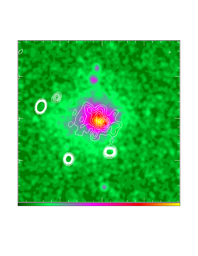
Figure 11: 1400-MHz radio contours superimposed on a soft X-ray image of Abell 2163 (Herbig & Birkinshaw 1995). Note the close resemblance of the radio and X-ray structures, and the diffuseness of the radio source. This is a particularly luminous example of a cluster radio halo source, with a radio luminosity $L_{\rm radio}\approx 10^{35}\,h_{100}^{-2}\ \rm W$.

As was noted in Sec. 3.3, a non-thermal population of electrons must also scatter microwave background photons, and it might be expected that a sufficiently dense relativistic electron cloud would also produce a Sunyaev-Zel’dovich effect. Fig. 11, which shows a radio map of Abell 2163 superimposed on a soft X-ray image, indicates that in some clusters there are populations of highly relativistic electrons (in cluster radio halo sources) that have similar angular distributions to the populations of thermal electrons which are more conventionally thought of as producing Sunyaev-Zel’dovich effects. Indeed, in many of the clusters in which Sunyaev-Zel’dovich effects have been detected there is also evidence for radio halo sources, so it is of interest to assess whether the detected effects are in fact from the thermal or the non-thermal electron populations.

Quick calculations based on the Kompaneets approximation (for example, equation 59), suggest that at low frequencies the amplitude of the Sunyaev-Zel’dovich effect should be

$${\Delta T_{\rm RJ}} = -2\,y\,{T_{\rm rad}}$$ (78)

$$= -2\,{T_{\rm rad}}\,\int{{k_{\rm B}}{T_{\rm e}}\over m_{\rm e}c^{2}}\,n_{\rm e}\,\sigma_{\rm T}\,dl$$

$$= -2\,{\sigma_{\rm T}\over m_{\rm e}c^{2}}\,\int p_{\rm e}dl$$

so that the effect depends on the line-of-sight integral of the electron pressure alone. If a radio halo source, such as is seen in Fig. 11, and the cluster gas which (presumably) confines it are in approximate pressure balance, then this argument would suggest that the thermal and non-thermal contributions to the overall Sunyaev-Zel’dovich effect should be of similar amplitude if the angular sizes of the radio source and the cluster gas are similar. Since the spectra of the thermal and non-thermal effects are distinctly different (compare Fig. 7 and 8), the spectrum of the overall Sunyaev-Zel’dovich effect measures the energy densities in the thermal gas and in the radio halo source separately. This would remove the need to use the minimum energy argument (Burbidge 1956) to deduce the energetics of the source.

Matters are significantly more complicated if the full relativistic formalism of Sec. 3 is used. But this is necessary, since the electrons which emit radio radiation by the synchrotron process are certainly highly relativistic and the use of the Kompaneets approximation is invalid. Thus we must distinguish between the effects of the electron spectrum and those of the electron scattering optical depth, but the results of Sec. 3.3 can be used to predict the expected Sunyaev-Zel’dovich effect intensity and spectrum from any particular radio source.

Consider, for example the Abell 2163 radio halo, for which we assume a spectral index $\alpha=-1.5$ (there is no information on the spectral index, since the halo has been detected only at 1400 MHz: $\alpha=-1.5$ is typical of radio halo sources). The diameter of the halo is about $1.2\,h_{100}^{-1}$ Mpc, and the radio luminosity (in an assumed frequency range from 10 MHz to 10 GHz) is $10^{35}\,h_{100}^{-2}\ \rm W$. Using the minimum energy argument in its traditional form (see the review by Leahy 1990), the equipartition magnetic field is about $0.06h_{100}^{2/7}\ \rm nT$ and the energy density in relativistic electrons is about $10^{-15}h_{100}^{4/7}\ \rm W\,m^{-3}$. This estimate assumes that all the particle energy resides in the electrons, and that the source is completely filled by the emitting plasma. The equivalent electron density in the source is $n_{\rm e}=2\times 10^{-3}\,h_{\rm 100}^{6/7}\ \rm m^{-3}$, which is a factor $\sim 10^{6}$ less than the electron density in the embedding thermal medium and corresponds to a scattering optical depth of only $6\times 10^{-9}\,h_{100}^{-1/7}$, which is certainly much less than the optical depth of the thermal atmosphere in which the radio source resides. Although the power-law electron distribution is more effective at scattering the microwave background radiation than the intracluster gas, at low frequencies it is found that the predicted Sunyaev-Zel’dovich effect from the halo radio source electron distribution is ${\Delta T_{\rm RJ}}=-5\ \rm nK$. This is about $10^{5}$ times smaller than the Sunyaev-Zel’dovich effect from the thermal gas.

The dominance of the thermal over the non-thermal effect from the cluster arises principally from the lower density of relativistic than non-relativistic electrons. Only a low relativistic electron density is inferred because of the high efficiency of the synchrotron process if only a small range of electron energies is present. If the frequency range of the synchrotron radiation is extended beyond the 10 MHz to 10 GHz range previously assumed, then the optical depth to inverse-Compton scattering depends on the lower frequency limit as $\tau_{\rm e}\approx 10^{-12}\,h^{-1/7}\,(\nu_{\rm min}/{\rm GHz})^{-13/7}$ (which would be $\gg 1$ if the electron spectrum extends down to thermal energies). A reduction in the lower cutoff frequency of the spectrum by a factor $\sim 10^{3}$ then increases the estimated relativistic electron density to the point that the non-thermal Sunyaev-Zel’dovich effect makes a significant contribution. Indeed, this strong dependence of $\tau_{\rm e}$ on $\nu_{\rm min}$ or, equivalently, on the minimum electron energy, suggests that the non-thermal Sunyaev-Zel’dovich effect is a potential test for the low-end cutoff energy of the relativistic electron spectrum.

Thus although the original purpose of searching for the non-thermal Sunyaev-Zel’dovich effect (as was done by McKinnon, Owen & Eilek 1990) was to check on the applicability of the minimum energy formula, it is more appropriate to think of it as a measurement of the minimum energy of the electrons that produce the radio radiation. Although limits on this minimum energy can be deduced from the polarization properties of radio sources, these limits are model-dependent (e.g., Leahy 1990), and an independent check from the non-thermal Sunyaev-Zel’dovich effect would be useful.

The problem of detecting the Sunyaev-Zel’dovich effect from non-thermal electron populations is likely to be severe because of the associated synchrotron radio emission. At low radio frequencies, that synchrotron emission will easily dominate over the small negative signal of the Sunyaev-Zel’dovich effect. At high radio frequencies, or in the mm-wave bands, there is more chance that the Sunyaev-Zel’dovich effect could be detectable, but even here there are likely to be difficulties separating the Sunyaev-Zel’dovich effects from the flattest-spectrum component of the synchrotron emission.

Several inadvertent limits to the non-thermal Sunyaev-Zel’dovich effect are available in the literature, from observations of clusters of galaxies which contain powerful radio halo sources (such as Abell 2163) or radio galaxies (such as Abell 426), but few detailed analyses of the results in terms of the non-thermal effect have been possible, and a treatment of the interpretation of the Abell 2163 data is deferred until later (Sec. 9.2).

Only a single intentional search for the Sunyaev-Zel’dovich effect from a relativistic electron population has been attempted to date (McKinnon et al. 1990), and that searched for the Sunyaev-Zel’dovich effect in the lobes of several bright radio sources. No signals were seen, but a detailed spectral fit of the data to separate residual synchrotron and Sunyaev-Zel’dovich effect signals was not done, and the limits on the Sunyaev-Zel’dovich effects (of $y\lesssim 2\times 10^{-3}$ for the best two sources) do not constrain the electron populations in the radio lobes strongly: the lobes could be far from equipartition without violating the Sunyaev-Zel’dovich effect constraint.

One difficulty with the analysis given above, and the discussion of the testing of minimum electron energy or the minimum energy formalism, is that radio sources are expected to be strongly inhomogeneous, so single-dish Sunyaev-Zel’dovich effect observations are averaging over a wide variety of different radio source structures (such as lobes and hot spots). This would mean, for example, that the spectral curvature that might be predicted by a superposition of the source spectrum and the Sunyaev-Zel’dovich effect might be also be produced by small variations in the electron energy distribution function from place to place within the radio source. If strong tests of the electron energy distribution are to be made, the observations must be made with angular resolution comparable with the scale of structures within the radio sources. For all but the largest radio sources (such as the lobes of Cen A), this means that interferometers (or bolometer arrays on large mm-wave telescopes) must be used. No work of such a type has yet been attempted, and the sensitivity requirements for a successful detection are formidable.

6 The kinematic Sunyaev-Zel’dovich effect

Although early work on the Sunyaev-Zel’dovich effects concentrated on the thermal effect, a second effect must also occur when the thermal (or non-thermal) Sunyaev-Zel’dovich effect is present. This is the velocity (or kinematic) Sunyaev-Zel’dovich effect, which arises if the scattering medium causing the thermal (or non-thermal) Sunyaev-Zel’dovich effect is moving relative to the Hubble flow. In the reference frame of the scattering gas the microwave background radiation appears anisotropic, and the effect of the inverse-Compton scattering is to re-isotropize the radiation slightly. Back in the rest frame of the observer the radiation field is no longer isotropic, but shows a structure towards the scattering atmosphere with amplitude proportional to $\tau_{\rm e}{v_{\rm z}\over c}$, where $v_{\rm z}$ is the component of peculiar velocity of the scattering atmosphere along the line of sight (Sunyaev & Zel’dovich 1972; Rephaeli & Lahav 1991).

The most interesting aspect of the kinematic effect is that it provides a method for measuring one component of the peculiar velocity of an object at large distance, provided that the velocity and thermal effects can be separated, as they can using their different spectral properties. Since there is evidence for large-scale motions of clusters of galaxies in the local Universe, both from COBE (Fixsen et al. 1996) and from direct observations of galaxies (e.g., Dressler et al. 1987; Lynden-Bell et al. 1988), and these motions place strong constraints on the dynamics of structure formation (see the review of Davis et al. 1992), other examples of large-scale flows would be of considerable interest. This is particularly true if those flows can be measured over a range of redshifts, so that the development of the peculiar velocity field can be studied. At present this is beyond the capability of the measurements (Sec. 8), but rapid progress is being made in this area.

Even larger velocities are possible for scattering gas: radio source lobes may be moving at speeds that approach the speed of light, and expanding at hundreds or thousands of ${\rm km\,s^{-1}}$. Although this will boost the kinematic effect, the optical depths of these lobes are probably too small to make the effect observable at present (Sec. 5; Molnar 1998).

Although Sunyaev & Zel’dovich (1972) quoted the result that the radiation temperature decrease in the kinematic effect is

$${\Delta{T_{\rm rad}}\over{T_{\rm rad}}}\approx-\tau_{\rm e}{v_{\rm z}\over c}$$ (79)

and the spectrum of the kinematic effect has often been quoted (e.g., by Rephaeli 1995b), the first published derivation of the size and spectrum of the kinematic effect was given by Phillips (1995). The version of the derivation given here is similar to Phillips’ argument, but uses different conventions and the radiative transfer equation (19) rather than the Boltzmann equation.

For the sake of simplicity, it is assumed that the kinematic and the thermal effects are both small, and that only single scatterings are important. Then the thermal effect, which depends on random motions of the scattering electrons, and the kinematic effect, which depends on their systematic motion, will decouple and we can derive the kinematic effect by taking the electrons to be at rest in the frame of the scattering medium. This approximation will ignore quantities which involve cross-products $\left({{k_{\rm B}}{T_{\rm e}}\over{m_{\rm e}}c^{2}}\right)\left({v_{\rm z}\over c}\right)$ relative to terms of order $\left({{k_{\rm B}}{T_{\rm e}}\over{m_{\rm e}}c^{2}}\right)$ and $\left({v_{\rm z}\over c}\right)$. Since the peculiar velocities and electron temperatures are small for the thermal Sunyaev-Zel’dovich effect, this will not be a significant limitation on the result for clusters of galaxies. However, this approximation is not valid for the non-thermal effect, where electron energies $\gg m_{\rm e}c^{2}$ are likely, and an alternative analysis is necessary (Molnar 1998; Nozawa et al. 1998).

In the rest frame of the CMBR, the spectrum of the radiation follows (1), and the occupation number has the form (15). The occupation number in mode $\alpha$ in a frame moving at speed $v_{\rm z}$ along the $z$ axis away from the observer is then

$$n_{\alpha}=\left(\exp{\left(x_{1}\gamma_{\rm z}(1-\beta_{\rm z}\mu_{1})\right)}-1\right)^{-1}$$ (80)

where $x_{1}={h\nu_{1}\over{k_{\rm B}}T_{1}}$ is the dimensionless frequency of photons in the frame of the scattering medium, the radiation temperature of the CMBR as seen by an observer at rest in the Hubble flow near the scattering gas is $T_{1}={T_{\rm rad}}(1+z_{\rm H})$, $z_{\rm H}$ is the Hubble flow redshift, and $\beta_{\rm z}=v_{\rm z}/c$ measures the peculiar velocity. $\gamma_{\rm z}$ is the corresponding Lorentz factor. $\mu_{1}=\cos\theta_{1}$ is the direction cosine of photons arriving at a scattering electron, relative to the $z$ axis and measured in the frame of the moving scattering medium (Fig. 12). The relativistic transformation of frequency relates $\nu_{1}$ to $\nu$ in the frame at rest relative to the CMBR by $\nu_{1}=\gamma_{\rm z}(1+\beta_{\rm z})\nu$, since the observer at rest sees the scattered photons along the $z$ axis, where $\mu=\cos\theta=1$.

We may apply the Boltzmann equation (e.g., as in Peebles 1993, Sec. 24 and Phillips 1995), or the radiative transfer equation (19), to derive an equation for the scattered radiation intensity. Using (19), and the form (24) for the scattering redistribution function, the specific intensity is given by

$${dI_{\nu_{1}}(\mu)\over d\tau_{\rm e}}=\int_{-1}^{+1}d\mu_{1}\,\phi(\mu,\mu_{1})\,\biggl{(}I_{\nu_{1}}(\mu_{1})-I_{\nu_{1}}(\mu)\biggr{)}\quad.$$ (81)

The optical depth, $\tau_{\rm e}$, enters from (19) as $\tau_{\rm e}=\int\alpha_{\nu,\rm sca}dz$. For small optical depth, so that photons are scattered only once, this can be simplified to

$${I_{\nu_{1}}(\tau_{\rm e};\mu)-I_{\nu_{1}}(0;\mu)\over\tau_{\rm e}}=\int_{-1}^{+1}d\mu_{1}\,\phi(\mu,\mu_{1})\,\biggl{(}I_{\nu_{1}}(0;\mu_{1})-I_{\nu_{1}}(0;\mu)\biggr{)}.$$ (82)

where the optical depth is now inserted as an explicit argument of $I$. For $\mu=1$, the scattering redistribution function takes a particularly simple form, and we can write the fractional change in the specific intensity in the frame of the scattering gas as

$${\Delta I_{\nu_{1}}\over I_{\nu_{1}}}=\tau_{\rm e}\,\int_{-1}^{+1}d\mu_{1}{3\over 8}(1+\mu_{1}^{2})\left({I_{\nu_{1}}(0;\mu_{1})\over I_{\nu_{1}}(0;1)}-1\right).$$ (83)

The expression on the left-hand side of this equation is a relativistic invariant: the same fractional intensity change would seen by an observer in the rest frame of the CMBR at frequency $\nu$, where $\nu$ is related to $\nu_{1}$ by a Lorentz transform. Furthermore, this is also the fractional intensity change seen by a distant observer, for whom the scattering medium lies at redshift $z_{\rm H}$, after allowance is made for the redshifting of frequency and radiation temperature. Using the expression for $n_{\alpha}$ in (80), and working in terms of the frequency seen at redshift zero, $\nu$, (83) becomes

$${\Delta I_{\nu}\over I_{\nu}}=\tau_{\rm e}\,\int_{-1}^{+1}d\mu_{1}\,{3\over 8}(1+\mu_{1}^{2})\,\left({e^{x}-1\over e^{x_{2}}-1}-1\right).$$ (84)

where $x_{2}=x\gamma_{\rm z}^{2}(1+\beta_{\rm z})(1-\beta_{\rm z}\mu_{1})$ and $x={h\nu\over{k_{\rm B}}{T_{\rm rad}}}$ as usual.

For small $\beta_{\rm z}$, the integral can be expanded in powers of $\beta_{\rm z}$, and the symmetry of the integrand ensures that only terms in the expansion which are even powers of $\mu_{1}$ will appear in the result. This enables the integral to be performed easily, giving the result

$${\Delta I_{\nu}\over I_{\nu}}=-\tau_{\rm e}\,\beta_{\rm z}\,{x\,e^{x}\over e^{x}-1}$$ (85)

so that the changes in specific intensity and brightness temperature are given by

$$\Delta I = -\beta\,\tau_{\rm e}\,I_{0}\,{x^{4}e^{x}\over\left(e^{x}-1\right)^{2}}$$ (86)

$${\Delta T_{\rm RJ}} = -\beta\,\tau_{\rm e}\,{T_{\rm rad}}\,{x^{2}e^{x}\over\left(e^{x}-1\right)^{2}}\quad.$$ (87)

This spectral form corresponds to a simple decrease in the radiation temperature (79), as stated by Sunyaev & Zel’dovich (1972).

For the cluster CL 0016+16 discussed in Sec. 4, the X-ray data imply a central scattering optical depth $\tau_{e0}=0.01h_{100}^{-1/2}$. At low frequency the brightness temperature change through the cluster center caused by the kinematic effect is $-\tau_{\rm e0}\,(v_{\rm z}/c)\,{T_{\rm rad}}=-0.1\,(v_{\rm z}/1000\ {\rm km\,s^{-1}})\,h_{100}^{-1/2}\ {\rm mK}$, significantly less than the central thermal Sunyaev-Zel’dovich effect of $-0.82h_{100}^{-1/2}\ {\rm mK}$ for all likely $v_{\rm z}$.

It would be very difficult to locate the kinematic Sunyaev-Zel’dovich effect in the presence of the thermal Sunyaev-Zel’dovich effect at low frequency. The ratio of the brightness temperature changes caused by the effects is

$${\Delta T_{\rm kinematic}\over\Delta T_{\rm thermal}} = {1\over 2}\,{v_{\rm z}\over c}\,\left({{k_{\rm B}}{T_{\rm e}}\over{m_{\rm e}}c^{2}}\right)^{-1}$$ (88)

$$= 0.085\,(v_{\rm z}/1000\ {\rm km\,s^{-1}})\,({k_{\rm B}}{T_{\rm e}}/10\ {\rm keV})^{-1}$$

which is small for the expected velocities of a few hundred ${\rm km\,s^{-1}}$ or less, and typical cluster temperatures of a few ${\rm keV}$. However, the thermal and kinematic effects may be separated using their different spectra: indeed, in the Kompaneets approximation it is easy to show that the kinematic effect produces its maximum intensity change at the frequency at which the thermal effect is zero.

Thus observations near $x=3.83$ ($218\ {\rm GHz}$) are sensitive mostly to the kinematic effect, but in interpreting such observations it is necessary to take careful account of the temperature-dependence of the shape of the thermal Sunyaev-Zel’dovich effect’s spectrum, and of the frequency of the null of the thermal effect (Equation 60; Fig. 9), as emphasized by Rephaeli (1995a). The first strong limits on the peculiar velocities of clusters of galaxies derived using this technique are now becoming available (e.g., Holzapfel et al. 1997b; see Sec. 10.2).

Although this technique measures only the peculiar radial velocity of a cluster of galaxies, the other velocity components may be measured using the specific intensity changes caused by gravitational lensing (e.g., Birkinshaw & Gull 1983a, corrected by Gurvits & Mitrofanov 1986; Pyne & Birkinshaw 1993). These fractional intensity changes are small, of order $\theta_{\rm grav}\,(v_{\rm xy}/c)$, where $\theta_{\rm grav}$ is the gravitational lensing angle, and $v_{\rm xy}$ is the velocity of the cluster across the observer’s line of sight. For typical cluster masses and sizes, the gravitational lensing angle is less than about 1 arcmin, so that $(\Delta I/I)\lesssim 10^{-6}\,(v_{\rm xy}/1000\ {\rm km\,s^{-1}})$, whereas the kinematic Sunyaev-Zel’dovich effect may be an order of magnitude stronger. The possibility of measuring $v_{\rm z}$ and $v_{\rm xy}$ separately then depends on the different angular patterns of the effects on the sky: the transverse motion produces a characteristic dipole-like effect near the moving cluster, with an angular structure which indicates the direction of motion on the plane of the sky. Nevertheless, substantial improvements in techniques are going to be required to measure these other velocity terms in this way.

Clusters of galaxies produce further microwave background anisotropies through the same spacetime effect, if they are expanding or contracting (Nottale 1984; Pyne & Birkinshaw 1993). A contaminating Sunyaev-Zel’dovich effect must also appear at the same time if an expanding or collapsing cluster contains associated gas because of the anisotropy of inverse-Compton scattering (Molnar & Birkinshaw 1998b), but the sizes of these effects are too small to be detectable in the near future.

An interesting extension of this work would be to use the kinematic Sunyaev-Zel’dovich effect from a radio source to measure the speed of the radio-emitting plasma. Just as for a cluster of galaxies, the presence of a scattering medium which is moving relative to the CMBR will produce a kinematic Sunyaev-Zel’dovich effect which is proportional to $\tau_{\rm e}\,(v_{\rm z}/c)$, but whereas $v_{\rm z}$ should be small for a cluster relative to the Hubble flow, the velocity of the radio-emitting plasma in a radio galaxy may be a substantial fraction of the speed of light, and a large kinematic Sunyaev-Zel’dovich effect will be seen if the optical depth of the radio-emitting plasma is sufficient. A complication here is that the location of the null of the non-thermal Sunyaev-Zel’dovich effect depends on the spectrum of the electrons, and that the cross-terms between the electron energy and the plasma velocity are no longer small. Thus the approximation of a cold plasma that was made in the derivation above, to calculate the spectrum of the kinematic Sunyaev-Zel’dovich effect, is no longer valid and a more complete calculation must be performed using proper angular averages over the (anisotropic) electron distribution function (see Molnar 1998).

7 Polarization and the Sunyaev-Zel’dovich effect

In the previous sections of this review I have concentrated on the Sunyaev-Zel’dovich effects in the specific intensity, the Stokes $I$ parameter. Any effects in the polarized intensity, the Stokes $Q$, $U$, and $V$ terms, will be of smaller order by factors $\tau_{\rm e}$, or $v/c$. An early reference was made to polarization terms in the paper by Sunyaev & Zel’dovich (1980b), with particular reference to their use to measure the velocities of clusters of galaxies across the line of sight. A more thorough discussion of polarization effects in inverse-Compton scattering is given by Nagirner & Poutanen (1994). All the polarization terms depend on higher powers of $\tau_{\rm e}$, $v_{\rm xy}$, or $v_{\rm z}$ than the thermal (or non-thermal) and kinematic effects discussed earlier, and therefore are not detectable with the current generation of experiments, although they may be measured in the future.

The simplest polarization term arises from multiple scatterings of photons within a scattering atmosphere. If a plasma distribution lies in front of a radio source, then the scattering of unpolarized radiation from that source by the surrounding atmosphere will produce a polarized halo, with the fractional polarization proportional to $\tau_{\rm e}$ but depending on the detailed geometry of the scattering process. For a radio source located centrally behind a spherical atmosphere, the pattern of polarization is circumferential. Similarly, scattering of the thermal (or non-thermal) Sunyaev-Zel’dovich effect by the same plasma producing the effect will produce a polarization, which may be circumferential (at high frequencies, where the Sunyaev-Zel’dovich effect appears as a source) or radial (at low frequencies, where it appears as a “hole”). The peak polarization in this case will be less than a fraction $\tau_{\rm e}$ of the Sunyaev-Zel’dovich effect itself, or less than $\tau_{\rm e}y$ relative to the overall CMBR. For the particularly prominent cluster CL 0016+16 (Sec. 4), this factor is $\approx 2\times 10^{-6}h_{100}^{-1}$, so that polarized signals of order $1\ {\rm\mu K}$ are the most that might be expected.

The motion of the plasma cloud across the line of sight also introduces polarization effects, from the Thomson scattering of the anisotropic radiation field in the frame of the moving cluster. The two largest contributions to the polarized intensity in this case were identified by Sunyaev & Zel’dovich (1980b) as a component of about $0.1\,\tau_{\rm e}\,(v_{\rm xy}/c)^{2}$ of the CMBR intensity, due to single scatterings of the quadrupolar term in the anisotropic radiation field seen in the frame of the moving cluster, and a component of about $0.025\,\tau_{\rm e}^{2}\,(v_{\rm xy}/c)$ from repeated scatterings of the dipolar term in the radiation field. Taking CL 0016+16 as an example again, the first of these polarizations is roughly a fraction $3\times 10^{-9}\,h_{100}^{-1/2}\,(v_{\rm xy}/1000\ {\rm km\,s^{-1}})^{2}$ of the intensity of the CMBR, while the second is of order $3\times 10^{-8}\,h_{100}^{-1}\,(v_{\rm xy}/1000\ {\rm km\,s^{-1}})$ of the CMBR intensity. Neither signal is likely to be measurable in the near future.

Similar effects will arise in the case of the non-thermal Sunyaev-Zel’dovich effect, but here the anisotropy of the electron distribution function is likely to be more significant. Polarized synchrotron radiation is also likely to be a bad contaminating signal for observational studies of the Sunyaev-Zel’dovich effect from relativistic populations of electrons.

No useful observational limits have yet been set on these polarization terms, and considerable development of observational techniques would be needed to make possible the measurement of even the largest of these effects.

8 Measurement techniques

Three distinct techniques for the measurement of the Sunyaev-Zel’dovich intensity effects in clusters of galaxies are now yielding reliable results. This section reviews single-dish radiometric observations, bolometric observations, and interferometric observations of the effects, emphasizing the weaknesses and strengths of each technique and the types of systematic error from which they suffer. A discussion of the constraints on observation of the non-thermal effect is contained in the discussion of bolometric techniques. No concerted efforts at measuring the polarization Sunyaev-Zel’dovich effects have yet been made, and so only intensity-measuring techniques will be addressed here.

8.1 Single-dish radiometer measurements

The original technique used to detect the Sunyaev-Zel’dovich effects made use of existing radio telescopes on which large tranches of observing time could be obtained. This always meant the older single-dish telescopes, so that the measurements were made using traditional radiometric methods. This is exemplified by the early work of Gull & Northover (1976) using the Chilbolton 25-m telescope, or the more recent work of Uson (1986) on the NRAO 140-foot telescope. These telescopes tend to have beam-sizes of a few arcminutes at microwave frequencies, which is a fairly good match to the angular sizes of the moderately distant clusters of galaxies which X-ray astronomy was then beginning to study. With such large and general-purpose telescopes, it was impossible to make major modifications that would optimize them for observations of the microwave background radiation, and much early work had to cope with difficulties caused by the characteristics of the telescopes through minor changes to the receiver package or careful design of the observing strategy.

The closest clusters of galaxies (at redshifts less than about $0.05$) have larger angular sizes, and it is possible to observe the Sunyaev-Zel’dovich effects using smaller telescopes. In such cases is has been possible to rework existing antennas to optimize them for microwave background observations — both of the Sunyaev-Zel’dovich effects and primordial structures (for example, using the OVRO 5.5-m telescope; Myers et al. 1997). This is now leading to a generation of custom-designed telescopes for sensitive measurements of the CMBR: some ground-based and some balloon-based systems should be in use in the near future.

A simple estimate of the sensitivity of a single-dish observation is of interest. A good system might have a noise temperature of about $40$ K (including noise from the atmosphere) and a bandwidth of $1$ GHz. Then in 1 second, the radiometric accuracy of a simple measurement will be $0.9$ mK, and a differenced measurement, between the center of a cluster of galaxies and some reference region of blank sky, would have an error of $1.3$ mK. Thus if problems with variations in the atmosphere are ignored, it would appear that a measurement with an accuracy of $10\ {\rm\mu K}$ could be made in 4.4 hours.

This observing time estimate is highly optimistic, principally because of emission from the Earth’s atmosphere. Sensitive observations with large or small single dishes always use some differencing scheme in order to reduce unwanted signals from the atmosphere (or from the ground, appearing in the sidelobes of the telescope) to below the level of the astronomical signal that is being searched for. Consider, for example, observations at 20 GHz, for which the atmospheric optical depth may be $\sim 0.01$ in good conditions at a good site. The atmospheric signal will then be of order $3\ {\rm K}$, several thousand times larger than the Sunyaev-Zel’dovich effects, and atmospheric signals must be removed to a part in $10^{5}$ if precise measurements of the Sunyaev-Zel’dovich effects are to be made.

The simplest scheme for removing the atmospheric signal is simply to position-switch the beam of an antenna between the direction of interest (for example the center of some cluster) and a reference direction well away from the cluster. The radiometric signals measured in these two directions are then subtracted. If the atmospheric signal has the same brightness at the cluster center as at the reference position, then it is removed, and the difference signal contains only the astronomical brightness difference between the two positions. Thus the reference position is usually chosen to be offset in azimuth, so that the elevations and atmospheric path lengths of the two beams are as similar as possible.

Of course, the sky in the target and reference directions will be different because of variations in the properties of the atmosphere with position and time, and because of the varying elevation of the target as it is tracked across the sky. Nevertheless, if the target and reference positions are relatively close together, the switching is relatively fast, and many observations are made, it might be expected that sky brightness differences between the target and reference positions would average out with time. The choice of switching angle and speed is made to try to optimize this process, while not spending so much time moving the beams that the efficiency of observation is compromised.

An alternative strategy is to allow the sky to drift through the beam of the telescope or to drive the telescope so that the beam is moved across the position of the target. The time sequence of sky brightnesses produced by such a drift or driven scan is then converted to a scan in position, and fitted as the sum of of a baseline signal (usually taken to be a low-order polynomial function of position) and the Sunyaev-Zel’dovich effect signal associated with the target. Clearly, structures in the atmosphere will cause the baseline shape to vary, but provided that these structures lie on scales larger than the angular scale of the cluster, they can be removed well by this technique. Many scans are needed to average out the atmospheric noise, and this technique is often fairly inefficient, because the telescope observes baseline regions far from the cluster for much of the time.

In practice these techniques are unlikely to be adequate, because of the amplitude of the variations in brightness of the atmosphere with position and time: at most sites the sky noise is a large contribution to the overall effective noise of the observation. Nevertheless, the first reported detection of a Sunyaev-Zel’dovich effect (towards the Coma cluster, by Parijskij 1972) used a simple drift-scanning technique, with a scan length of about $290$ arcmin and claimed to have measured an effect of $-1.0\pm 0.5$ mK.

More usually a higher-order scheme has been employed. At cm wavelengths, it is common for the telescope to be equipped with multiple feeds so that two or more directions on the sky can be observed without moving the telescope. The difference between the signals entering through these two feeds is measured many times per second, to yield an “instantaneous” beam-switched sky signal. On a slower timescale the telescope is position-switched, so that the sky patch being observed is moved between one beam and the other. At mm wavelengths it is common for the beam switching to be provided not by two feeds, but by moving the secondary reflector, so that a single beam is moved rapidly between two positions on the sky. This technique would allow complicated differencing strategies, if the position of the secondary could be controlled precisely, but at present only simple schemes are being used. Arrays of feeds and detectors are now in use on some telescopes, and differencing between signals from different elements of these feed arrays also provide the opportunity for new switching strategies (some of which are already being used in bolometer work, see Sec. 8.2).

Table 1, which reports the critical observing parameters used in all published radiometric observations of the Sunyaev-Zel’dovich effects, indicates the switching scheme that was used. Most measurements have been made using a combination of beam-switching (BS) and position-switching (PS), because this is relatively efficient, with about half the observing time being spent on target. Some observations, including all observations by the Effelsberg group, have used a combination of beam-switching and drift or driven scanning (DS). The critical parameters of these techniques are the telescope beamwidth (the full width to half maximum, FWHM), $\theta_{\rm h}$, the beam-switching angle, $\theta_{\rm b}$, and the angular length of the drift or driven scan, $\theta_{\rm s}$. Some of the papers in Table 1 have been partially or fully superseded by later papers, and are marked $\ast$.

In techniques that use a combination of beam-switching and position switching, the beam and position switching directions need not be the same, and need bear no fixed relationship to any astronomical axes. However, the commonest form of this technique (illustrated in Fig. 13) has the telescope equipped with a twin-beam receiver with the two beams offset in azimuth. Since large antennas are usually altazimuth mounted, it is convenient also to switch in azimuth (and so keep the columns of atmosphere roughly matched between the beams). In any one integration interval (typically some fraction of a second) the output of the differential radiometer is proportional to the brightness differences seen by the two beams (possibly with some offset because of differences in the beam gains, losses, etc.). The configuration used by Readhead et al. (1989) in their observations of primordial anisotropies in the microwave background radiation is typical. In the simplest arrangement, where the two beams (A and B) are pointed towards sky positions $1$ and $2$, and the signals from the feeds enter a Dicke switch, followed by a low-noise front-end receiver, and then are synchronously detected by a differencing backend, the instantaneous output of the radiometer, $\Delta P$, was written by Readhead et al. as

$$\Delta P = \phantom{+}G\biggl{(}g_{\rm A}(1-l_{\rm A})T_{\rm sky1}-g_{\rm B}(1-l_{\rm B})T_{\rm sky2}\biggr{)}$$ (89)

$$+G\biggl{(}g_{\rm A}(1-l_{\rm A})(T_{\rm atm1}+T_{\rm gndA})-g_{\rm B}(1-l_{\rm B})(T_{\rm atm2}+T_{\rm gndB})\biggr{)}$$

$$+G\biggl{(}g_{\rm A}\int\Theta_{\rm A}dl_{\rm A}-g_{\rm B}\int\Theta_{\rm B}dl_{\rm B}\biggr{)}$$

$$+G\biggl{(}(g_{\rm A}-g_{\rm B})T_{\rm maser}\biggr{)}\quad.$$

Here $G$ is the gain of the front-end system (a maser in the OVRO 40-m telescope configuration used by Readhead et al.), with an equivalent noise temperature of $T_{\rm maser}$. $g_{\rm A}$ and $g_{\rm B}$ are the back-end gains corresponding to the A and B (main and reference) feeds, and $l_{\rm A}$ and $l_{\rm B}$ are the losses in the feeds, waveguides, and Dicke switch associated with the two channels. These losses are distributed over a number of components, with temperatures $\Theta_{\rm A}$ and $\Theta_{\rm B}$ which range from the cryogenic temperatures of the front-end system to the ambient temperatures of the front of the feeds.

It is clear that the instantaneous difference power between channels A and B may arise from a number of causes other than the sky temperature difference $(T_{\rm sky1}-T_{\rm sky2})$ which it is desired to measure. In general, the atmospheric signal greatly exceeds the astronomical signal towards any one position on the sky ($T_{\rm atm1}\gg T_{\rm sky1}$) so that small imbalances in the atmospheric signal between the two beams dominate over the astronomical signals that are to be measured. Over long averaging times, and with the same zenith angle coverage in the two beams, it is expected that $\langle T_{\rm atm1}-T_{\rm atm2}\rangle\approx 0$. The accuracy with which this is true will depend on the weather patterns at the telescope, the orientation of the beams relative to one another, and so on.

The ground pickup signals through the two beams are likely to be different, since the detailed shapes of the telescope beams are also different. This leads to an imbalance $T_{\rm gndA}-T_{\rm gndB}$, and an offset signal in the radiometer. The amplitude of this signal is reduced to a minimum by tapering the illumination of the primary antenna, so that as little power as possible arrives at the feed from the ground. Some protection against ground signals is also achieved by operating at elevations for which the expected spillover signal is smallest. However, since the ground covers a large solid angle there are inevitably reflection and diffraction effects that cause offsets from differential ground spillover.

The losses $l_{\rm A}$ and $l_{\rm B}$ in the two channels of the radiometer are reduced to a minimum by keeping the waveguide lengths to a minimum and using the best possible microwave components, but it is impossible to ensure that the losses are equal. Furthermore, the temperatures of the components in which these losses occur depend critically on where they are in the radiometer housing, so that the radiated signals from the components, $\int\Theta_{\rm A}dl_{\rm A}$ and $\int\Theta_{\rm B}dl_{\rm B}$ are likely to be significantly different. Once again, this produces an offset signal between the two sides of the radiometer.

These problems are exacerbated by their time variations. It is likely that the gains and temperatures will drift with time. The receiver parameters are stabilized as well as possible, but are still seen to change slowly. The atmosphere and ground pickup temperatures change more significantly, with varying weather conditions and varying elevations of the observation. Thus simple beam-switched measurements of the Sunyaev-Zel’dovich effect are unlikely to be successful, even after filtering out periods of bad weather and rapid temperature change when the atmospheric signal is unstable.

The level of differencing introduced by position-switching removes many of these effects to first order in time and position on the sky. The standard position-switching technique points one beam (A, the “main beam”) at the target position for time $\tau$, with the second beam (B, the “reference beam”) offset in azimuth to some reference position, then switches the reference beam onto the target for time $2\tau$, with the main beam offset to a reference position on the opposite side of the target, then switches back for a final time $\tau$ with the original beam on the target. If the total cycle time ($4\tau+s_{1}+s_{2}$, where $s_{1}$ and $s_{2}$ are the times spent moving) is small, then the reference positions observed by beams A and B do not change appreciably during a cycle, and the combination

$$S={1\over\tau}\int_{0}^{\tau}\Delta Pdt-{2\over\tau}\int_{\tau+s_{1}}^{3\tau+s_{1}}\Delta Pdt+{1\over\tau}\int_{3\tau+s_{1}+s_{2}}^{4\tau+s_{1}+s_{2}}\Delta Pdt$$ (90)

is a much better measurement of the sky temperature difference between the target and the average of two points to either side of it (offset in azimuth by the beam-switching angle, $\theta_{\rm b}$) than the estimate in (89). This is so even when the move and dwell times in the different pointing directions change slightly, for example because of variations in windage on the telescope. If $\tau$ is chosen to be small, then quadratic terms in the time and position variations of contaminating effects in (89) can be made very small, but at the cost of much reduced efficiency $4\tau/(4\tau+s_{1}+s_{2})$ in the switching cycle. For observations with the OVRO 40-m telescope made by Readhead et al. (1989) and Birkinshaw et al. (1998), $\tau$ was chosen to be about 20 sec, and even large non-linear terms in the telescope properties are expected to be subtracted to an accuracy of a few $\mu\rm K$.

Even at this degree of differencing, it is important to check that the scheme is functioning properly. For this reason, the best work has included either a check of regions of nominally blank sky near the target point, or a further level of differencing involving the subtraction of data from fields leading and following the target field by some interval. A representative method (Herbig et al. 1995) consists of making a few ($\sim 10$) observations using the beam-switching plus position switching technique described above at the target field, referenced to the same number of observations on offset regions before and after the target field, with the time interval arranged so that the telescope moves over the same azimuth and elevation track as the target source. The off-target data may be treated as controls, or may be directly subtracted from the on-target data to provide another level of switching which is likely to reduce the level of differential ground spillover. In either case, rigorous controls of this type necessarily reduce the efficiency of the observations by a factor 2 or 3. Alternatively, observations can be made of closer positions (perhaps even overlapping with the reference fields of the target point), without attempting an exact reproduction of the azimuth and elevation track on any one day, but allowing an equal coverage to build up over a number of days. This was the approach used by Birkinshaw et al. (1998).

The various beam switching schemes that have been used are described in detail in the papers in Table 1 that discuss substantial blocks of measurements. Quantitative estimates of their systematic errors from differential ground spillover, residual atmospheric effects, or receiver drifts, are also usually given. Whichever beam-switching technique is used, it is advisable to use the same technique to observe control fields, far from known X-ray clusters, where the expected measurement is zero. Systematic errors in the technique are then apparent, as is the extra noise in the data caused by primordial structures in the CMBR. It is important to realize that the Sunyaev-Zel’dovich effect plus primordial signal at some point can be measured to more precision than the systematic error on the Sunyaev-Zel’dovich effect that is set by the underlying spectrum of primordial fluctuations. That is, the measurement error is a representation of the reproducibility of the measurement, which is the difference between the brightness of some point relative to a weighted average of adjacent points. Noise from the spectrum of primordial fluctuations must be taken into account if realistic errors on physical parameters of a cluster are to be deduced from measured Sunyaev-Zel’dovich effect data.

A further difficulty encountered with single-dish observations is that of relating the measured signal from the radiometer (in volts, or some equivalent unit) to the brightness temperature of a Sunyaev-Zel’dovich effect on the sky. The opacity of the atmosphere can be corrected using tip measurements, and generally varies little during periods of good weather, so that the principal problem is not one of unknown propagation loss but rather one of calibration. Generally the absolute calibration of a single-dish system is tied to observations of planets, with an internal reference load in the radiometer being related to the signal obtained from a planet. If that planet has solid brightness temperature $T_{\rm p}$, then the output signal is proportional to $T_{\rm p}$, with a constant of proportionality which depends on the solid angle of the planet, the telescope beam pattern, etc. Thus by measuring the telescope beam pattern and the signal from planets, it is possible to calibrate the internal load. The accuracy of this calibration is only modest because of

1. measurement errors in the planetary signal, from opacity errors in the measurement of the transparency of the atmosphere, pointing errors in the telescope, etc.,

2. uncertainties in the brightness temperature scale of the planets, and in the pattern of brightness across their disks, and

3. variations in the shape of the telescope beam (and hence the gain) over the sky.

Thus, for example, the recent measurements of Myers et al. (1997) are tied to a brightness temperature scale using the measurement of the brightness temperature of Jupiter at 18.5 GHz (Wrixson, Wright & Thornton 1971). This measurement may itself be in error by up to 6 per cent. Difficulties may also arise from changes in the internal reference load, which will cause the calibration to drift with time. Relating this load back to sky temperatures at a later date will introduce another set of “transfer errors”. Even if these are well controlled, it is clear that radiometric Sunyaev-Zel’dovich effect data contain systematic uncertainties in the brightness scale at the 8 per cent level or worse. This calibration error has a significant effect on the interpretation of the results.

It is important to mention, at this stage, that the differencing schemes described here have the effect of restricting the range of redshifts for which the telescope is useful. If observations are to be made of a cluster of galaxies at low redshift, then the angular size of the cluster’s Sunyaev-Zel’dovich effects (which are several times larger than of the cluster’s X-ray surface brightness) may be comparable to the beam-switching angle, $\theta_{\rm b}$, and beam-switching reduces the observable signal. Alternatively, if the cluster is at high redshift, then its angular size in the Sunyaev-Zel’dovich effects may be smaller than the telescope FWHM, $\theta_{\rm h}$, and beam dilution will reduce the observable signal. The two effects compete, so that for any telescope and switching scheme, there is some optimum redshift band for observation, and this band depends on the structures of cluster atmospheres and the cosmological model. An example of a calculation of this efficiency factor, defined as the fraction of the central Sunyaev-Zel’dovich effect from a cluster that can be observed with the telescope, is shown in Fig. 14 for the OVRO 40-m telescope. The steep cutoff at small redshift represents the effect of the differencing scheme, while the decrease of the efficiency factor at large $z$ arises from the slow variation of angular size with redshift at $z\gtrsim 0.5$.

In dealing with the variations of signal during a tracked observation of a cluster, it is convenient to introduce the concept of parallactic angle, the angle between the vertical circle and the declination axis. An observation at hour angle $H$ of a source at declination $\delta$ from a telescope at latitude $\lambda$ will occur at parallactic angle

$$p=\tan^{-1}\left({\sin H/\cos\delta\over\tan\lambda-\tan\delta\cos H}\right)$$ (91)

where the parallactic angle increases from negative values to positive values as time increases (with the parallactic angle being zero at transit; Fig. 13) for sources south of the telescope, and decreases from positive values to negative values for sources north of the telescope. For a symmetrical beam-switching experiment, like that depicted in Fig. 13, the parallactic angle may be taken to lie in $-90^{\circ}$ to $+90^{\circ}$. With more complicated beam-switching schemes, which may be asymmetrical to eliminate higher-order terms in the time or position dependence (e.g., Birkinshaw & Gull 1984), the full range of $p$ may be needed.

The conversion between time and parallactic angle is particularly convenient when it is necessary to keep track of the radio source contamination. Many of the observations listed in Table 1 were made at cm wavelengths, where the atmosphere is relatively benign and large antennas are available for long periods. However, the radio sky is then contaminated by non-thermal sources associated with galaxies (in the target cluster, the foreground, or the background) and quasars, and the effects of these radio sources must be subtracted if the Sunyaev-Zel’dovich effects are to be seen cleanly.

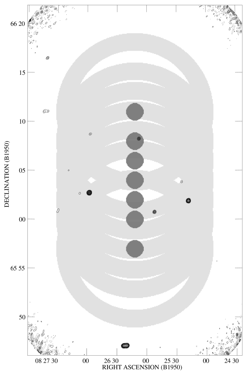
Figure 15: Observing positions and radio sources in the cluster Abell 665. The dark-grey circles represent the FWHMs of the primary pointing positions of the Birkinshaw et al. (1998) Sunyaev-Zel’dovich effect observations in the cluster, while the light-grey areas are the reference arcs traced out by the off-position beams. A VLA 6-cm radio mosaic of the cluster field is shown by contours. Note the appearance of a significant radio source under the pointing position 4 arcmin north of the cluster center. This source appears to be variable, causing significant problems in correcting the data at that location. Other radio sources appear near or within the reference arcs, and cause contamination of some parts of the data.

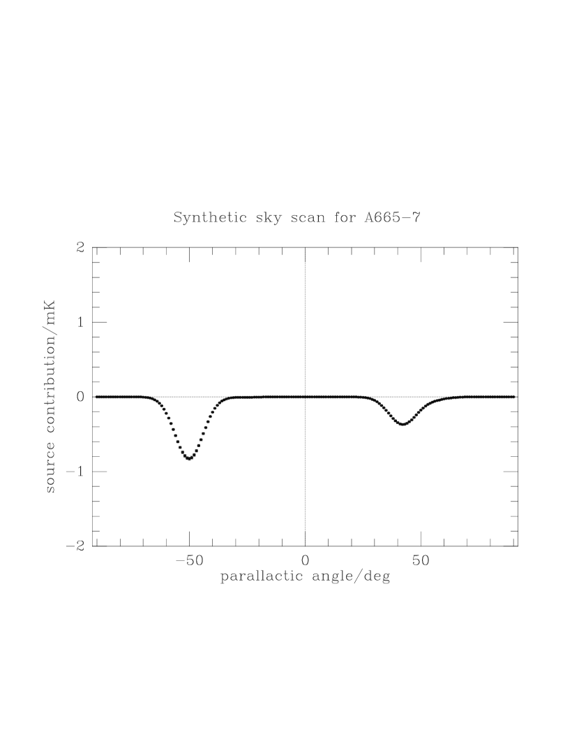
Figure 16: A comparison of the observed and modeled parallactic angle scans for OVRO 40-m data at a point 7 arcmin south of the nominal center of Abell 665. Two features are seen in the observed data (left). These correspond to bright radio sources which are seen in the reference arcs at parallactic angles near $-50^{\circ}$ and $40^{\circ}$ (position angles $+40^{\circ}$ and $-50^{\circ}$ on Figs 13 and 15). The model of the expected signal based on VLA surveys of the cluster (Moffet & Birkinshaw 1989) shows features of similar amplitude at these parallactic angles, so that moderately good corrections can be made for the sources. The accuracy of these source corrections is questionable because of the extrapolation of the source flux densities to the higher frequency of the Sunyaev-Zel’dovich effect data and the possibility that the sources are variable.

Figure 15 shows a map of the radio sky near Abell 665. Significant radio source emission can be found in the reference arcs of the observations at many parallactic angles. Such emission causes the measured brightness temperature difference between the center and edge of the cluster to be negative: a fake Sunyaev-Zel’dovich effect is generated. Protection against such fake effects is implicit in the differencing scheme. Sources in the reference arcs affect the Sunyaev-Zel’dovich effect measurements only for the range of parallactic angles that the switching scheme places them in the reference beam. A plot of observational data arranged by parallactic angle therefore shows negative features at parallactic angles corresponding to radio source contamination (e.g., Fig. 16), and data near these parallactic angles can be corrected for the contamination using radio flux density measurements from the VLA, for example.

This procedure is further complicated by issues of source variability. At frequencies above 10 GHz where most radiometric observations are made (Table 1), many of the brightest radio sources are variable with timescales of months being typical. Source subtraction based on archival data is therefore unlikely to be good enough for full radiometric accuracy to be recovered. Simultaneous, or near-simultaneous, monitoring of variable sources may then be necessary if accurate source subtraction is to be attempted, and this will always be necessary for variable sources lying in the target locations. Variable sources lying in the reference arcs may also be simply eliminated from consideration by removing data taken at the appropriate parallactic angles: thus in Fig. 16, parallactic angle ranges near $-50^{\circ}$ and $+40^{\circ}$ might be eliminated on the basis of variability or of an imprecise knowledge of the contaminating sources. However, sources which are so strongly variable that they appear from below the flux density limit of a radio survey will remain a problem without adequate monitoring of the field.

Despite difficulties with radio source contamination, calibration, and systematic errors introduced by the radiometer or spillover, recent observations of the Sunyaev-Zel’dovich effects using radiometric techniques are yielding significant and highly reliable measurements. The detailed results and critical discussion appear in Sec. 9, but a good example is the measurement of the Sunyaev-Zel’dovich effect of the Coma cluster by Herbig et al. (1995), using the OVRO 5.5-m telescope at 32 GHz. Their result, an antenna temperature effect of $-175\pm 21\ \rm\mu K$, corresponds to a central Sunyaev-Zel’dovich effect $\Delta T_{\rm T0}+\Delta T_{\rm K0}=-510\pm 110\ \rm\mu K$, and is a convincing measurement of the Sunyaev-Zel’dovich effect from a nearby cluster of galaxies for which particularly good X-ray and optical data exist (e.g., White, Briel & Henry 1993).

For a few clusters, single-dish measurements have been used not only to detect the central decrements, but also to measure the angular sizes of the effects. This is illustrated in Fig. 17 which, for the three clusters CL 0016+16, Abell 665, and Abell 2218 shows the Sunyaev-Zel’dovich effect results of Birkinshaw et al. (1998). The close agreement between the centers of the Sunyaev-Zel’dovich effects and the X-ray images of the clusters is a good indication that the systematic problems of single-dish measurements have been solved, although observing time limitations and the need to check for systematic errors restricts this work to a relatively coarse measurement of the cluster angular structure. Much better results should be obtained using two-dimensional arrays of detectors, as should be available on the Green Bank Telescope when it is completed.

8.2 Bolometric methods

The principal advantage of a bolometric system is the high sensitivity that is achieved, but these devices are also of interest because of their frequency range: at present they provide the best sensitivity for observing the microwave background outside the Rayleigh-Jeans part of the spectrum, and hence for separating the thermal and kinematic components of the Sunyaev-Zel’dovich effect using their different spectral shapes. Furthermore, the best systems consist of several detectors arranged in an array, and some provide simultaneous operation in several bands. A suitable choice of differencing between elements of the array reproduces many of the sky-noise subtraction properties of radiometric observing, and the multiband capability holds out the hope of rapid spectral measurements. Bolometric measurements of the Sunyaev-Zel’dovich effects are now becoming more common, as reliable technology becomes more widely available (Table2).

A bolometer such as SCUBA on the James Clerk Maxwell Telescope (JCMT) at a wavelength of $850\ \rm\mu m$ (near the peak of the thermal effect in intensity terms) has a sensitivity of $80\ \rm mJy\,Hz^{-1/2}$, with a 13-arcsec pixel size. The equivalent sensitivity in the Rayleigh-Jeans brightness temperature change of the thermal Sunyaev-Zel’dovich effect, ${\Delta T_{\rm RJ}}$, is about $60$ mK in one second in each pixel, or about 13 mK in a 1 arcmin beam created by averaging over detector elements (compare the radiometric sensitivity of a typical radio telescope in Sec. 8.1). A few hours of observation should then suffice to detect the thermal Sunyaev-Zel’dovich effect at high sensitivity, and by using several bands (perhaps simultaneously), a coarse spectrum of the effect could be measured. Deviations from the spectrum of the thermal effect could then set limits to the velocities of clusters of galaxies — if the sensitivity of the bolometer is similar at frequencies near the zero of the thermal effect, then a velocity accuracy of about $6\times 10^{4}\ {\rm km\,s^{-1}}$ can be achieved in an hour of observation in any one 13-arcsec pixel. This can be reduced to $10^{3}\ {\rm km\,s^{-1}}$ or less with modern bolometers if the measurements are averaged over the entire face of a cluster (as, for example, in Holzapfel et al. 1997b). The fundamental limit of this technique for measuring cluster peculiar velocities may be set not by sensitivity, but rather by the background fluctuations in the CMBR which arise from primordial anisotropies. This depends on the angular spectrum of anisotropies (see Sec. 1.3).

Although the raw sensitivity of bolometer systems is high because of the large bandpasses and sensitive detector elements, a problem with the technique is the extremely high sky brightness against which observations must be made. Coupled with the varying opacity of the sky, this implies that telescopes on high, dry, sites are essential for efficient observing — balloon operations are possible, and the CalTech Submillimeter Observatory (CSO) on Mauna Kea has been used successfully. Antarctic operations are also an interesting future possibility, as is space operation with bolometer arrays. At present, the best results are obtained by differencing out atmospheric signals using bolometer arrays. This involves the use of small differencing angles, and introduces limitations on the selection of clusters that are similar to those that apply to radiometric work (Sec. 8.1). The small angular separations of the beams often causes the minimum redshift cutoff to be rather high, and the peak observing efficiency to be low (as in Chase et al. 1987, for which the fraction of the central decrement that was observable was only 0.38 for cluster CL 0016+16).

This technique is exemplified by the recent work of Wilbanks et al. (1994), who used the Caltech Submillimeter Observatory (CSO) on Mauna Kea with a three-element array to detect the Sunyaev-Zel’dovich effect from Abell 2163, a cluster of galaxies with an exceptionally hot atmosphere (Arnaud et al. 1992) and a bright radio halo source (Herbig & Birkinshaw 1998). The combination of drift-scanning and element-to-element differencing used by Wilbanks et al. achieved an excellent separation of the atmospheric signal from the Sunyaev-Zel’dovich effect and provided a measurement of the angular structure of the effect. At the wavelength of operation ($\lambda=2.2$ mm) radio source confusion is not a problem. This is not the case at microwave frequencies, where observations of the Sunyaev-Zel’dovich effect in Abell 2163 are severely affected by the radio environment near the cluster center, which includes a variable and inverted-spectrum radio source as well as the radio halo (Herbig & Birkinshaw 1998). Nevertheless, recent observations at 18 GHz with the OVRO 40-m telescope have succeeded in detecting the effect near the cluster center, at about the level seen by Wilbanks et al. (1994).

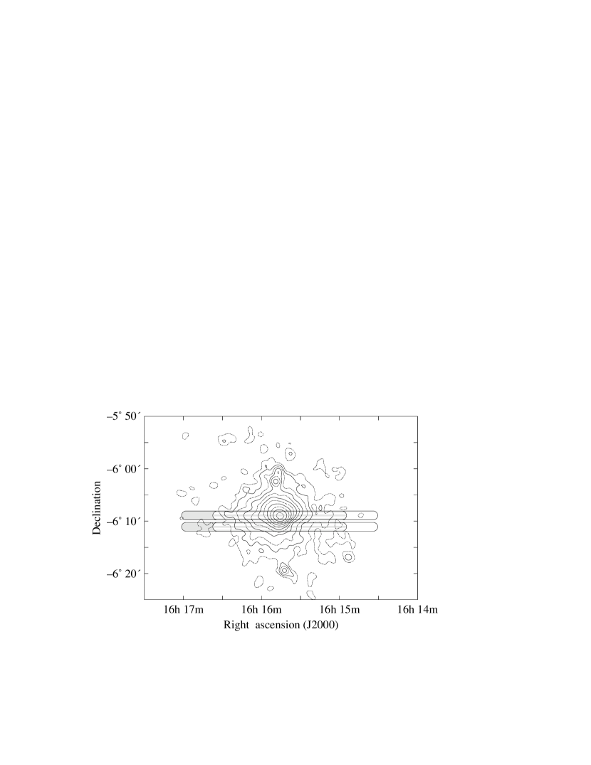
Figure 18: Sample SuZIE drift scans across Abell 2163 superimposed on an X-ray contour map of the cluster (Holzapfel et al. 1997a). The two rows of SuZIE detectors are separated by 2.2 arcmin, so that when the upper detectors pass over the X-ray center, the lower detectors pass south of the center. Two sets of scans are shown for each row of detectors, since the observations were alternately begun 12 and 18 arcmin ahead of the cluster center.

The most sensitive observations with bolometers (with SuZIE, the Sunyaev-Zel’dovich Infrared Experiment on the CSO) have been made using a drift-scan mode (Holzapfel et al. 1997a), as illustrated in Fig. 18, in order to reduce microphonic and sidelobe spillover effects to the minimum possible level. The SuZIE array consists of two rows of three elements, with the rows separated by 2.2 arcmin and the elements in each array separated by 2.3 arcmin. Array elements within a row are electronically differenced to produce continuous measurements of the brightness differences that they see. During a drift-scan each difference voltage is then proportional to the brightness difference on the sky between two locations which vary as the sky rotates past the detectors. The array is oriented with the long axis parallel to right ascension, so that the time series can be interpreted as a right ascension scan (as in Fig. 19). Repeated drift-scans, with the angle of the array changed from scan to scan, then allow repeated measurements of brightness differences at the same points on the sky.

A simple isothermal model of Abell 2163 (Holzapfel et al. 1997a) has $\beta=0.62\pm 0.03$ and ${\theta_{\rm c}}=1.2\pm 0.1$ arcmin (in equation 64). The 2.3 and 4.6-arcmin difference signals that SuZIE produces then correspond to peak observing efficiencies (fractions of the central Sunyaev-Zel’dovich effect seen by each 1.75-arcmin FWHM array element) of 0.31 and 0.51, respectively. With this type of observing, the signals returned by SuZIE are close to being measurements of the gradient of the Sunyaev-Zel’dovich effect on the sky, as can be seen in the data shown in Fig. 19.

Just as for radiometric work, it is important to check that the observing technique being used does not suffer from baseline effects from parasitic signals from the sky, the telescope, or the electronics. Control observations of regions of blank sky are used to provide such checks, as in the example of Fig. 19. In all plots in this figure, a best-fitting linear baseline has been removed, and then the data have been fitted using a model of the cluster Abell 2163: only small residual baseline effects remain, and the fits are of reasonable quality.

As with the radiometer data, it is important to remove from the data periods when the sky is opaque, or has rapidly-varying opacity, and the data must also be corrected for the line-of-sight opacity through the atmosphere. At the best millimetric wavelengths these corrections are small, just as they are for most cm-wave observations. Also, as radiometer data must be cleaned of radio interference, so bolometer data must be cleaned of cosmic ray hits. In both cases, this does not create additional difficulties because the effects are generally large and obvious.

A final similarity with radiometric work is the problem of calibrating the data into absolute temperature (or intensity) units. Again, the calibration is usually made by reference to the brightness of planets, and again the difficulty is that the planetary temperature scale is good to 6 per cent at best. Additional errors from the beam-pattern of the detectors, the bandpasses of the detector elements, and the opacity of the atmosphere add to this error, so that the intensity scale of any measurement is not known to better than about 8 per cent. The effect of this on the interpretation of the data will become apparent later.

No radio source or Galactic contamination signals are thought to be significant at the frequencies and angular resolutions at which bolometric data are taken on clusters (Fischer & Lange 1993), and dusty galaxies within the clusters should also be weak. Nevertheless, such signals are present (Smail, Ivison & Blain 1997), and may be enhanced by emission from distant (background) dusty, star-forming galaxies gravitationally lensed by clusters — especially by the massive clusters which produce the strongest Sunyaev-Zel’dovich effects (Blain 1998). If the bolometer array that is used has sufficient angular resolution, it should be possible to reduce this contamination by removing the individual pixels in the map that are affected, but at present only low-resolution bolometric observations of the Sunyaev-Zel’dovich effect exist (e.g., from SuZIE, with 1.7 arcmin resolution, Table 2). Higher-resolution observations of clusters (e.g., with SCUBA on the JCMT) are now possible and should allow checks for the presence of confusing sources, and then their subtraction from the lower-resolution data.

Since differencing in bolometric work usually involves switching over angles which are only a small multiple of the FWHM of the array elements, the observing efficiencies are low. This has led to the results from these experiments usually being quoted in terms of fitted central Sunyaev-Zel’dovich effects (or, equivalently, the $y$ parameter) rather than the beam-averaged central Sunyaev-Zel’dovich effect that is usually quoted in radiometric measurements. Quoting the results as central $y$ values has the virtue of encapsulating the combined statistics of the observational errors and the angular structure data (Fig. 19) into a single number, but it also has the drawback of not allowing the data to be re-interpreted later, as improved structural information becomes available. From the data in Fig. 19, Holzapfel et al. (1997a) find that Abell 2163 has a central Comptonization parameter $y=(3.7\pm 0.4)\times 10^{-4}$ if the cluster gas follows a simple isothermal model. The corresponding central Rayleigh-Jeans brightness temperature change is $-1.6\pm 0.2$ mK: a remarkably large Sunyaev-Zel’dovich effect, presumably because of the high temperature of the atmosphere in this cluster, although uncertainties in the model, which is based on X-ray data, cause additional $\sim 10$ per cent uncertainties in the values of $y$ and the central Sunyaev-Zel’dovich effect that are derived.

An interesting recent result on the spectrum of the Sunyaev-Zel’dovich effect from Abell 2163 is shown in Fig. 20 (Lamarre et al. 1998). Lamarre et al. combined data taken using several instruments into a single spectrum which shows the relative sizes of the Sunyaev-Zel’dovich effect and far-IR dust-like emission (which dominates from $100-1000\ \mu\rm m$). This shorter-wavelength emission may arise from the lensed population of background starburst galaxies, from Galactic dust which happens to be brighter near the centre of the cluster, or from dust in Abell 2163 itself. If the spectrum in Fig. 20 is characteristic of other clusters of galaxies, then the interpretation of sub-mm data will need to take careful account of such contamination. This might particularly affect the measurement of the kinematic Sunyaev-Zel’dovich effect.

8.3 Interferometric methods

The two techniques discussed provided most of the existing data on the Sunyaev-Zel’dovich effect until very recently. Both techniques are excellent for large-scale surveys of clusters of galaxies which are well matched to the beam-switching technique being used, but provide only modest angular resolutions on the sky (although higher-resolution and two-dimensional bolometer arrays are now becoming available) and hence are suitable only for simple mapping (as in Figs 17 and 19). Radio interferometry is a powerful method for making detailed images of Sunyaev-Zel’dovich effects. Such images are valuable for making detailed comparisons with X-ray images, and can also measure accurate Sunyaev-Zel’dovich effects while avoiding some of the systematic difficulties of the other techniques. Perhaps for these reasons, interferometry is the most rapidly-growing area for observation of the Sunyaev-Zel’dovich effects (Table 3).

The extra resolution that is available using interferometers is also a handicap. Interferometers work by measuring some range of Fourier components of the brightness distribution on the sky: the correlation of signals from a pair of antennas produces a response which is (roughly) proportional to a single Fourier component of the brightness of the source. For “small” sources, observed with narrow bandwidths and short time constants, the measured source visibility is

$${\cal V}(u,v)\propto\int_{-\infty}^{\infty}\,d\xi\,\int_{-\infty}^{\infty}\,d\zeta\,B(\xi,\zeta)\,G(\xi,\zeta)\,e^{-2\pi i(u\xi+v\zeta)}$$ (92)

where $B(\xi,\zeta)$ is the brightness distribution of the sky, $G(\xi,\zeta)$ represents the polar diagram of the antennas of the interferometer, $(u,v)$ are the separations of the antennas, measured in wavelengths, $(\xi,\zeta)$ are direction cosines relative to the center of the field of view, and the constant of proportionality depends on the detailed properties of the interferometer (see Thompson, Moran & Swenson (1986) for a detailed explanation of the meaning of this expression and the assumptions that go into it). An image of the sky brightness distribution, $B(\xi,\zeta)$, can be recovered from the measurements ${\cal V}(u,v)$, by a back Fourier transform and division by the polar diagram function: alternatively, estimation techniques can be used to measure $B(\xi,\zeta)$ directly from the ${\cal V}(u,v)$.

Most interferometers were originally designed to achieve high angular resolution. The finiteness of interferometer measurements means that not all $(u,v)$ values are sampled: in particular, the design for high resolution means that the antennas are usually placed so that their minimum separation is many wavelengths (and always exceeds the antenna diameter by a significant factor). The Fourier relationship (92) means that the short baselines contain information about the large angular scale structure of the source, and so there is some maximum angular scale of structure that is sampled and imaged by interferometers. The Sunyaev-Zel’dovich effects of clusters of galaxies have angular sizes of several arcminutes — most interferometers lose (“resolve out”) signals on these or larger angular scales, and hence would find extreme difficulty in detecting Sunyaev-Zel’dovich effects.

Figure 21 illustrates this effect for model Very Large Array (VLA) observations of cluster CL 0016+16 at $\lambda=6$ cm. Since the VLA antennas shadow one another at baselines less than the antenna diameter (of 25 m), no information about the amplitude or shape of the visibility curve can be recovered at baselines less than $420\lambda$. Most of the VLA baselines are much larger than the minimum baseline, even in the most compact configuration (D array). Hence the VLA’s effective sensitivity to the Sunyaev-Zel’dovich effect in CL 0016+16 is low. But CL 0016+16 is a cluster at redshift $0.5455$, has a small angular size, and so represents one of the best candidate clusters for observation with the VLA — the VLA is therefore not a useful instrument for measuring the Sunyaev-Zel’dovich effects of any clusters unless those clusters contain significant small-scale substructure in the Sunyaev-Zel’dovich effect, or the clusters can have significantly smaller angular sizes and substantial Sunyaev-Zel’dovich effects. Thus, for example, the VLA observations of Partridge et al. (1987) suffered from this effect: in their data the Sunyaev-Zel’dovich effect signal from Abell 2218 was strongly suppressed because of the excessive size of the array.

Smaller interferometers would allow the Sunyaev-Zel’dovich effects to be measured. What is needed is an array of antennas whose individual beam-sizes are significantly larger than the angular sizes of the cluster Sunyaev-Zel’dovich effects, so that many antenna-antenna baselines can be arranged to be sensitive to the effects. A first attempt to customize a telescope for this experiment was the upgrade of the 5-km telescope at Cambridge, UK into the Ryle telescope (Birkinshaw & Gull 1983b; Saunders 1995). In its new configuration, the five central 12.8-m diameter antennas can occupy a number of parking points which provide baselines from 18 m to 288 m. At the prime operating wavelength of 2 cm, the maximum detectable Sunyaev-Zel’dovich effect signal is about $-1.3\ {\rm mJy}$, and several baselines should see effects in excess of $-0.1$ mJy.

The choice of operating wavelength for mapping the Sunyaev-Zel’dovich effect is constrained to some extent by confusion, in the same way that the radiometric observations are affected. Some clusters of galaxies (particularly clusters of galaxies with strong Sunyaev-Zel’dovich effects; Moffet & Birkinshaw 1989) contain cluster halo sources, with similar angular size to the cluster as a whole and whose non-thermal radio emission can swamp the Sunyaev-Zel’dovich effects at low frequencies (although their non-thermal Sunyaev-Zel’dovich effects are probably small; Sec. 5). Such sources have steep spectra, and so are avoided by working at higher frequencies. Clusters of galaxies also contain a population of radio sources, many of which are extended (the wide angle tail sources, narrow angle tail sources, etc.). These extended sources are also avoided by working at high frequency, where their extended emission is minimized and where the small-scale emission can be recognized by its different range of Fourier components. Background, flat-spectrum, radio sources can also affect the data, but can be recognized by their small angular size.

Interferometers with a wide range of baselines are useful in this respect: the longer baselines are sensitive to the small-angular scale radio sources which dominate the radio confusion signal (and which affect the radiometric data: see Fig. 15), while the shorter baselines contain both the radio source signal and the Sunyaev-Zel’dovich effect signal. Thus the longer-baseline data can be analysed first to locate the confusing radio sources, and then these sources can be subtracted from the short-baseline data, so that a source-free map of the sky can be constructed and searched for the Sunyaev-Zel’dovich effect. Furthermore, by tuning the range of baselines that are included in the final map, or by appropriately weighting these baselines, a range of image resolutions can be produced to emphasize any of a range of angular structures.

Of course, this technique depends on there being a good separation of angular scales between the radio sources and the Sunyaev-Zel’dovich effects in the clusters: extended, cluster-based, radio sources cannot be removed reliably using this technique, and there are a number of clusters in which no good measurements of (or limits to) the Sunyaev-Zel’dovich effects can be obtained without working at a higher frequency with a smaller interferometer (to avoid resolving out the Sunyaev-Zel’dovich effect). A good choice of operating frequency might be 90 GHz, with antenna baselines of a few metres: a design which also commends itself for imaging primordial fluctuations in the background radiation.

Since many of the brightest radio sources at the frequencies for which interferometers are used are variable (with timescales of months being typical), the subtraction technique must sometimes be applied to individual observing runs on a cluster, rather than to all the data taken together. The brightest sources may also subtract imperfectly because of dynamic range problems in the mapping and analysis of the data: generally interferometric or radiometric observations of clusters are only attempted if the radio source environment is relatively benign. Any source contamination at a level $\gtrsim 10$ mJy is likely to be excessive, and to cause difficulties in detecting the Sunyaev-Zel’dovich effects, let alone mapping them reliably. Nevertheless, interferometric work has the advantage over radiometric work that the sources (in particular the variable, and hence small angular size sources) are monitored simultaneously with the Sunyaev-Zel’dovich effect, and so interferometer maps should show much better source subtraction.

Although the interferometric technique is extremely powerful, in taking account of much of the radio source confusion, and in allowing a map of the Sunyaev-Zel’dovich effect to be constructed, it does suffer from some new difficulties of its own. First, the range of baselines over which the Sunyaev-Zel’dovich effect is detected may be highly restricted, so that the “map” is little more than an indication of the location of the most compact component of the Sunyaev-Zel’dovich effects. This problem can only be solved by obtaining more short baselines, which may not be possible because of excessive antenna size (as with the VLA, for example).

The source subtraction may also cause problems, since strong sources outside the target clusters often lie towards the edges of the primary beam of the antennas of the interferometer. Small pointing errors in the antennas can then cause the amplitude of these sources to modulate significantly, adding to the noise in the map and reducing the accuracy with which the contaminating source signal can be removed from the Sunyaev-Zel’dovich effect. The problem is worst for sources lying near the half-power point of the primary beam, but significant difficulties can be caused by sources lying even in distant sidelobes, although this extra noise does not usually add to produce a coherent contaminating signal at the map center, where the Sunyaev-Zel’dovich effect is normally expected.

Careful attention must also be paid to the question of correlator errors, which can produce large and spurious signals near the phase-stopping center (see Partridge et al. 1987). In order to avoid excessive bandwidth smearing for contaminating sources which must be identified and removed successfully, it is also normal to observe using bandwidth synthesis methods (which split the continuum bandpass of the interferometer into a number of channels). The combination of these individual channel datasets back into a continuum map of the Sunyaev-Zel’dovich effect may sometimes be complicated by steep (or strongly-inverted) sources on the image which have different fluxes in the different channels.

One major advantage of using an interferometer is that the effects of structures in the atmosphere are significantly reduced. Emission from the atmosphere is important only in its contribution to the total noise power entering the antennas, since this emission is uncorrelated over baselines longer than a few metres and does not enter into the (correlated) visibility data. Furthermore, there are no background level problems: an interferometer does not respond to a constant background level, and so a well-designed interferometer will not respond to constant atmospheric signals, the uniform component of the microwave background radiation, large-scale gradients in galactic continuum emission, or ground emission entering through the telescope sidelobes.

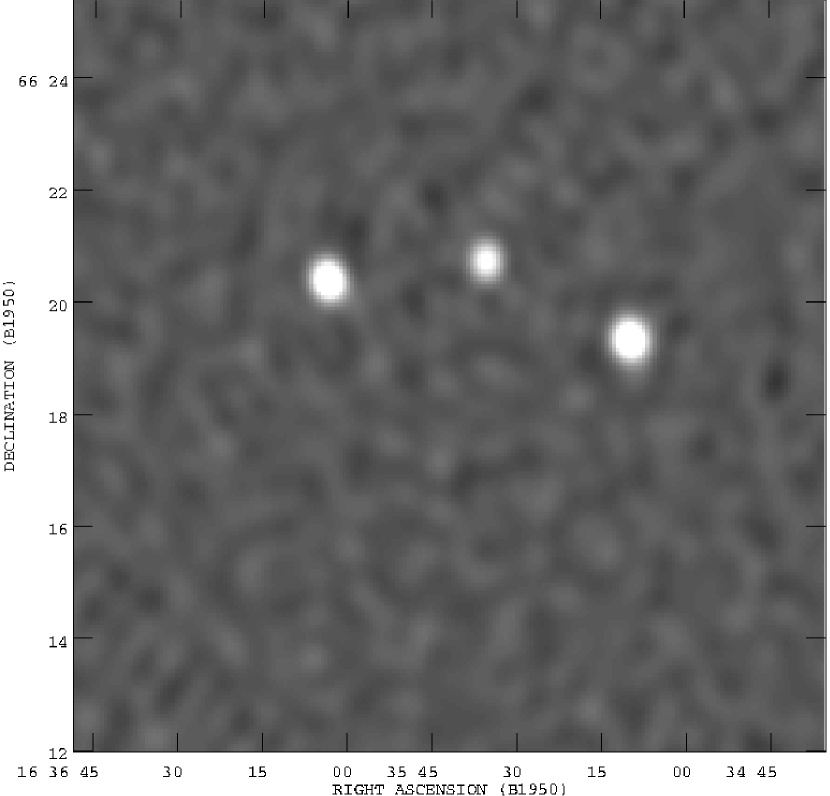
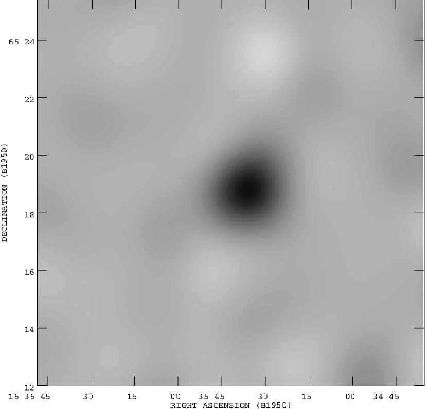
Figure 22: Interferometric maps of Abell 2218, made with the Ryle telescope of the Mullard Radio Astronomy Observatory (Jones et al. 1993). Left: an image made with the longer-baseline data, which is sensitive chiefly to small angular scales. Three faint radio sources dominate the image. Right: an image made with the short-baseline data, after subtraction of the sources detected on the long-baseline image. Here the image is dominated by the Sunyaev-Zel’dovich effect from the cluster.

The first cluster for which interferometric techniques were used successfully is Abell 2218, which had been shown to have a strong Sunyaev-Zel’dovich effect with a small angular size using single-dish measurements (Birkinshaw, Gull & Hardebeck 1984). Jones et al. (1993) used the Ryle interferometer at 15 GHz, with baselines from 18 to 108 m, to locate sources and to map the diffuse Sunyaev-Zel’dovich effect. The images that they obtained are shown in Fig. 22. Using baselines from 36 to 108 m, and 27 12-hour runs, a high signal/noise map of the cluster radio sources was made (Fig. 22, left). Using only the 18-m baseline, and subtracting the signals from these sources, a map with effective angular resolution about 2 arcmin was then made (Fig. 22, right). This clearly shows a significant negative signal, of $-580\pm 110\ \rm\mu Jy$, centered at $\rm 16^{h}35^{m}47^{s}$ $+66^{\circ}12^{\prime}50^{\prime\prime}$ (J2000). The corresponding value for the central Sunyaev-Zel’dovich effect in the cluster cannot be determined without knowing the shape of the efficiency curve (e.g., Fig. 21, which is effectively a visibility curve) on baselines less than those that were observed. The Ryle interferometer data could be fitted with models of the form (66), with a parameter space extending from $\beta\simeq 0.6$, ${\theta_{\rm c}}\simeq 0.9$ arcmin, $\Delta T_{0}\simeq-1.1$ mK, to $\beta\simeq 1.5$, ${\theta_{\rm c}}\simeq 2.0$ arcmin, $\Delta T_{0}\simeq-0.6$ mK. The random error on the detection of an Sunyaev-Zel’dovich effect is, therefore, much smaller than the systematic error in the central measurement of the effect — a better range of baselines, and a detection of the Sunyaev-Zel’dovich effect on more than a single baseline, would be needed to improve this situation.

Much analysis of the Sunyaev-Zel’dovich effect can usefully be carried out in the data, rather than the map, plane — by fitting the model ${\cal V}(u,v)$ to the measured visibilities. Indeed, the most reliable indication of the reality of a Sunyaev-Zel’dovich effect may be its presence first in visibility plots (like Fig. 21), and such plots are invaluable for assessing the extent of the missing visibility data in $(u,v)$, and hence the fraction of the full Sunyaev-Zel’dovich effect of a cluster that is being detected by the interferometer. Of course, similar calculations are needed for radiometric and bolometric observations of the Sunyaev-Zel’dovich effects, but the efficiency factors $\eta(b)$ are often lower in interferometric work, and so the sampling of the full Sunyaev-Zel’dovich effect is more critical to its interpretation.

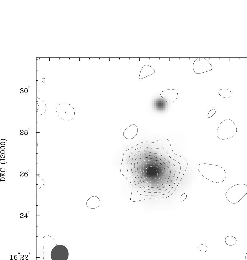
Figure 23: An interferometric map of CL 0016+16, from Carlstrom et al. (1996), superimposed on a grey-scale representation of the X-ray emission of the cluster (from the ROSAT PSPC). The radio data on which this image is based were taken with the Owens Valley Radio Observatory Millimeter Array operated at 1 cm, contain antenna baselines from 20 to 75 m, and have a synthesized beam of about $55$ arcsec (as shown in the lower left corner).

More recently, excellent imaging data on the clusters CL 0016+16 and Abell 773 has been published by Carlstrom, Joy & Grego (1996). These authors used the Owens Valley Millimeter Array (OVMMA) at 1 cm: by equipping an array designed for operation at 3 mm and shorter wavelengths with cm-wave receivers, they were assured of accurate pointing and a relatively large primary beam, so that the interferometer should not over-resolve the Sunyaev-Zel’dovich effects on short baselines. The total negative flux density of CL 0016+16 in this operating configuration is near $-13$ mJy if the cluster has a central decrement of $-1$ mK, so that the cluster should be relatively strong (negative) source. With the OVMMA, Carlstrom et al. (1996) detected a total negative flux density of $-3.0$ mJy after 13 days of observation: their map of the cluster is shown in Fig. 23.

The power of radio interferometric mapping of a cluster is apparent in Carlstrom et al.’s map of the Sunyaev-Zel’dovich effect from CL 0016+16. The Sunyaev-Zel’dovich decrement is extended in the same position angle as the X-ray emission (Fig. 2) and the distribution of optical galaxies (and close to the position angle from the cluster to a companion cluster; Hughes et al. 1995). The small-scale structure seen in this image is close to that predicted from the X-ray image, and corresponds closely with the predicted amplitude based on earlier radiometric detections of the Sunyaev-Zel’dovich effect of the cluster (Uson 1986; Birkinshaw 1991).

The success of recent interferometric mapping campaigns, which have produced results such as Fig. 24 has amply justified demonstrated the potential of this technique to improve on single-dish observations of the Sunyaev-Zel’dovich effect. The critical elements of this breakthrough have been the development of small interferometers dedicated to Sunyaev-Zel’dovich effect mapping over long intervals, and the existence of stable, low-noise receivers with exceptionally wide passbands.

9 Sunyaev-Zel’dovich effect data

The techniques discussed in Section 8 have been used to search for the thermal and kinematic Sunyaev-Zel’dovich effects towards a large number of clusters, and the non-thermal Sunyaev-Zel’dovich effects towards a few radio galaxies. Over the past few years this work has been increasingly successful, because of the high sensitivity that is now being achieved, and the careful controls on systematic errors that are used by all groups. The most impressive results are those obtained from radio interferometers, which are producing images of the cluster Sunyaev-Zel’dovich effects that can be compared directly with images of cluster X-ray structures. In the present section I collect all published results on Sunyaev-Zel’dovich effects of which I am aware, and review the reliability of the measurements.

9.1 Cluster data

Table 4 contains the final result measured in each series of observations for each of the clusters that has been observed in the Sunyaev-Zel’dovich effect. Not all papers in Tables 1, 2, and 3 are represented in Table 4, since I have excluded interim reports where they have been superseded by later work (which often involves improved calibrations and assessments of systematic errors). The column marked “O/C” reports whether the quoted value of ${\Delta T_{\rm RJ}}$ is as observed or as deconvolved, by the observers, into some central estimated Sunyaev-Zel’dovich effect. As explained in Secs 8.2 and 8.3, model-fitting to produce a central decrement is commonly used when only a small fraction of the central decrement can be recorded by the telescope.

The overall set of clusters for which Sunyaev-Zel’dovich effects have been sought does not constitute a well-defined sample in any sense. Early work on the Sunyaev-Zel’dovich effects concentrated on clusters with strong X-ray sources, or for which the radio source contamination was known to be small. Abell 426 (the Perseus cluster) is an example of a cluster observed for the first reason, despite its strong radio sources (Lake & Partridge 1980). Abell 665, on the other hand, was observed principally because it was known to be largely free of strong radio sources, but also because it is the richest cluster in the Abell catalogue (Birkinshaw et al. 1978a). With more sensitive X-ray surveys, X-ray images, and X-ray spectroscopy, several clusters with exceptional X-ray properties have also been observed. Examples are the high-luminosity cluster CL 0016+16 (Birkinshaw et al. 1981a), and the high-temperature cluster Abell 2163 (Holzapfel et al. 1997b).

More recently, there has been some effort to observe complete samples of clusters of galaxies selected on the basis of their X-ray or optical properties, since the interpretation of cluster Sunyaev-Zel’dovich effects in cosmological terms may be biased by the use of the ad hoc samples that have been assembled to date. Initial steps in these directions have been taken by, for example, Myers et al. (1997). At present, though, it is not possible to use the sample of clusters contained in Table 4 to make reliable statistical statements about the effects of clusters on the CMBR. Attempts to normalize a Sunyaev-Zel’dovich effect cluster luminosity function (e.g., Bartlett & Silk 1994a) based on these clusters may not be safe.

Extreme care is needed in interpreting the results given in this table. First, the datum that is recorded, ${\Delta T_{\rm RJ}}$, is the measured Sunyaev-Zel’dovich effect from the cited paper at the most significant level observed (code O), or the central Sunyaev-Zel’dovich effect in the cluster, as fitted based on some model of the cluster gas (code C), and which would be seen in the Rayleigh-Jeans limit if the cluster were observed with infinitely good angular resolution. That is, for C codes,

$${\Delta T_{\rm RJ}}=-2\,{T_{\rm rad}}\,y_{0}\quad.$$ (93)

It is not simple to convert from the measured effects to the central effects, since proper account must be taken of the method used to observe the cluster and the efficiency factor $\eta$ (see Fig. 14, for example). For some observations, for example with multichannel bolometer systems, it may have been necessary for the observers to undertake a significant fitting exercise to extract the central ${\Delta T_{\rm RJ}}$, ${\Delta T_{\rm RJ0}}$, with the result depending on the model of the cluster gas adopted (Sec. 8.2). Clusters with only poor X-ray images are therefore difficult to assess, but in cases in which there is good X-ray data this fitting step is relatively reliable. Thus it can be shown, for example, that recent results for Abell 2218 are in much better agreement than is apparent from Table 4 (see later).

Many of the observations made with bolometers express their results in terms of $y_{0}$, the central value of $y$ through the target cluster. In those cases (e.g., Holzapfel et al. 1997b), I have converted the results to central decrements using (93). In cases where the peak beam-averaged value of ${\Delta T_{\rm RJ}}$ is stated (e.g., Chase et al. 1987), that value is preferred in the table.

For the interferometric data, the measured flux densities on the most appropriate (usually lowest-resolution) maps have been converted into measured brightness temperatures using the synthesized beamsize quoted. That is, it is assumed that the synthesized beam is an elliptical Gaussian, with solid angle $\Omega_{\rm ab}$ (calculated from the full widths to half-maximum in two directions, $h_{\rm a}\times h_{\rm b}$), and the brightness temperature is obtained from

$$\Delta S_{\nu}=2\,{k_{\rm B}}\,{\Delta T_{\rm RJ}}\,\left({\Omega_{\rm ab}\over\lambda^{2}}\right)$$ (94)

which in convenient units, becomes

$$({\Delta T_{\rm RJ}}/{\rm\mu K})=340\,(\Delta S/{\rm\mu Jy}\ {\rm beam^{-1}})\,(\nu/{\rm GHz})^{-2}\,(h_{\rm a}/{\rm arcmin})^{-1}\,(h_{\rm b}/{\rm arcmin})^{-1}.$$ (95)

In the case of the Partridge et al. (1987) data, I have estimated the error on the central Sunyaev-Zel’dovich effect from their visibility curves, taking rough account of the systematic errors in the data caused by correlator offsets.

For the radiometric results, which are the bulk of the entries in Table 4, the values of ${\Delta T_{\rm RJ}}$ are taken directly from the papers. The results from Rudnick (1978) are given for a 2-arcmin FWHM structure at the cluster center, since this is the closest match to the resolution of the telescope used. Rudnick also quotes more sensitive results for ${\Delta T_{\rm RJ}}$ at a number of larger angular scales by convolving the data. These larger scales may be more appropriate for some clusters.

In many cases the radiometric data have been adjusted for the effects of cluster and background radio sources. These adjustments are not necessarily consistent between the different papers: as further radio work has been done on the clusters, some have shown that substantial radio source corrections are needed (see, for example, Abell 2507). Sometimes the detections of these radio sources led to the cluster observations being abandoned (e.g., for Abell 426). For other clusters, later work may have used better source corrections and is often more reliable on these grounds alone. Many of the clusters with radiometric Sunyaev-Zel’dovich results reported here have had little supporting work on the radio source environment. This makes it difficult to assess the extent to which the results are affected by radio source contamination.

A number of trends are clear in Table 4. Early observations were dominated by single-dish radiometers (e.g., Birkinshaw et al. 1981b). More recently, the bolometric technique has been used, specially because of the interest in detecting the effect near 190 GHz, where the kinematic effect is more obvious (e.g., Holzapfel et al. 1997b). Finally, the completion of the Ryle array and the use of the OVMMA and BIMA for Sunyaev-Zel’dovich effect measurements has produced a series of sensitive maps of clusters (e.g., Jones et al. 1993; Carlstrom et al. 1996), where some evidence of the cluster structure is seen (e.g., for CL 0016+16; Carlstrom et al. 1996; Sec. 8.3).

Despite the increasing use of these new techniques, single-dish radiometry is still used — principally for survey work, to locate target clusters with significant Sunyaev-Zel’dovich effects that might be the subjects of detailed mapping later. Thus observations at OVRO with the 40-m telescope at present are concentrating on a sample of clusters selected because of their excellent exposures by the ROSAT PSPC. Myers et al. (1997) are making a survey of another sample of clusters with the OVRO 5.5-m telescope.

The results in Table 4 span more than 20 years of work on the Sunyaev-Zel’dovich effect, and involve a number of different techniques with different observing characteristics. Thus it is difficult to compare the results of different groups for any one cluster without taking detailed account of the structure of the cluster and the details of the method used. This causes the apparent disagreements between different groups’ results to be accentuated. Nevertheless, there are clusters for which the data (particularly the more recent data) are largely in agreement, and clusters for which the situation is less clear.

Consider, for example, the cluster Abell 2218, for which a particularly large number of measurements are available. First, consider the history of results for Abell 2218 obtained by the group with which I have been working. The published results from 1976 to 1996 are given in Table 5. These results are not independent: later results from the Chilbolton 25-m telescope included the data used in earlier papers, and the OVRO 40-m results also changed as more data were accumulated, and as the radio source corrections and data calibrations were better understood.

The internal consistency of the early data is clearly poor. The final result based on the Chilbolton data is only marginally consistent with the first published result, suggesting that the later data were quite inconsistent with the earlier data. Since a number of changes in the configuration of the Chilbolton system occurred during the period that data were taken, it is likely that this inconsistency arose from unrecognized systematic errors, possibly involving strong ground signals entering through distant sidelobes.

Later data, from the OVRO 40-m telescope, appear more consistent — the 10.7-GHz result and the 20.3-GHz results seem to be indicating that the value of ${\Delta T_{\rm RJ}}$ towards the center of the cluster is about $-0.35$ mK. However, the observing characteristics of these observations was very different, and the low-significant detection at 10.7 GHz is due almost completely to a correction for contaminating radio sources near the center of the cluster.

If it is assumed that the atmosphere of Abell 2218 follows the model (64), and is isothermal, then the structural parameters $\beta=0.65\pm 0.05$ and ${\theta_{\rm c}}=1.0\pm 0.1$ arcmin derived from X-ray observations (Birkinshaw & Hughes 1994) may be used to calculate the efficiencies with which the cluster was observed by any telescope. For observations of the Sunyaev-Zel’dovich effect of Abell 2218 with the Chilbolton 25-m telescope, the OVRO 40-m telescope at 10.7 GHz, and the OVRO 40-m telescope at 20.3 GHz, these efficiencies are about $0.35$, $0.49$, and $0.60$, respectively. The inferred central Sunyaev-Zel’dovich effects from the cluster according to the final results from these three telescope configurations are therefore $-3.0\pm 0.6$, $-0.77\pm 0.38$, and $-0.67\pm 0.08$ mK. The result from the Chilbolton 25-m telescope is clearly inconsistent with the other two measurements. Only a very contrived structure for the cluster atmosphere could cause such differences and be consistent with the other Sunyaev-Zel’dovich effect data and the X-ray image and spectrum. Thus an economical assumption is that the early data were badly contaminated by systematic errors, and should be discarded, and that the true central decrement from Abell 2218 is near $-0.7$ mK.

Another effect that can be seen in Table 5 is the strong variation in the errors quoted for the 20.3-GHz data as a function of time. The smallest error ($\pm 0.03$ mK, in Birkinshaw & Moffet 1986) represents the error on the data accumulated at that time if all the data are considered to be drawn from a single, static, Gaussian distribution. The largest error, $\pm 0.13$ mK, in Birkinshaw & Gull (1984), is based on the smallest amount of data, under the same assumptions. On the other hand, the entry for Birkinshaw (1986) is based on substantially more data than in Birkinshaw & Moffet (1986), but includes a generous allocation for possible systematic errors. Later entries in the Table include further data, and were derived with detailed analyses for systematic errors. It should be noted that the final result in the table, $-0.40\pm 0.05$ mK, contains no contribution from the background CMBR anisotropies, so that the error represents the reproducibility of the measurement rather than the external error that would be achieved if Abell 2218 could be observed against another patch of the background radiation.

Of course, Table 5 illustrates principally the difficulty in measuring the Sunyaev-Zel’dovich effect signals in the presence of systematic errors with unknown characteristics: reductions in the error are principally achieved by stronger controls against systematic errors (for example by observing multiple regions of blank sky, performing checks for radio source contamination, and so on). More rigorous controls against systematic error are obtained by comparing the results from different groups who observe the same cluster in different ways. The most frequently-observed cluster is Abell 2218, and Table 6 lists the central decrements for Abell 2218 deduced from 16 independent measurements using the same model atmosphere as in discussion of Table 5.

It is at once apparent from Table 6 that the individual results are inconsistent: the early data are often scattered with dispersion several times their nominal error about the later data. In some of the early papers, large parasitic signals from ground spillover have been removed (e.g., Perrenod & Lada 1979), but there remains a suspicion that residual systematic errors are present in the data. Overall, the later data are in much better agreement. A notable exception is the result of Klein et al. (1991), where the measured decrement is consistent with predictions based on other data, but its location on the sky is far from the X-ray center of the cluster so that the implied central decrement in Table 6 is unrealistically large. If an average is taken over these data, and the most obviously discordant results are excluded, then the central decrement in Abell 2218 is found to be $-0.74\pm 0.07$ mK. The error here has been increased to take some crude account of the remaining discordance in the data (the value of $\chi^{2}=15$ with 10 degrees of freedom).

The Sunyaev-Zel’dovich effect results for Abell 2218 are generally in better agreement now than they were for the first few years of reported measurements. This suggests that several groups are now able to measure reliable Sunyaev-Zel’dovich effects, and based on this conclusion, I have collected into Table 7 the set of all Sunyaev-Zel’dovich effects that I believe are both significant (at $>4\sigma$) and reliable. These objects constitute a set for which a simultaneous analysis of the Sunyaev-Zel’dovich effect data and the X-ray data may provide useful constraints on the cluster atmospheres (Sec. 10), and possibly a measurement of the Hubble constant (Sec. 11). Of the thirteen clusters in the table, seven were first detected using single-dish radiometers, two using bolometers, and four using interferometers. Only four of these detections have independent confirmations at significance $>4\sigma$. Much work remains to be done to measure the Sunyaev-Zel’dovich effects in these clusters, and all three measurement techniques still have their place in Sunyaev-Zel’dovich effect research, although bolometer measurements are becoming more important, and interferometric maps of the effect are probably the most reliable.

Detections at lower significance exist for more objects, including the lines of sight towards two high-redshift quasars (PHL 957, Andernach et al. 1986; PC 1643+4631, Jones et al. 1997). These detections may arise from distant clusters of galaxies along the lines of sight, or from the host clusters of the quasars themselves, or from some other cause. However, if the Sunyaev-Zel’dovich effects arise from line-of-sight objects, then observations towards “blank” sky regions should show Sunyaev-Zel’dovich effects as often as observations towards the quasars — it is not yet clear whether this is the case, so the interpretation of these Sunyaev-Zel’dovich effects and the limits from observations of other quasars (Jones et al. 1997) or blank fields (Richards et al. 1997) is at present obscure.

Further complications in the interpretation of these results have arisen as deep optical and X-ray followups have been made. Thus for the PC 1643+4631 field, Saunders et al. (1997) find no cluster that might be responsible for a Sunyaev-Zel’dovich effect in deep optical images, and Kneissl, Sunyaev & White (1998) find no X-ray emission associated with hot gas. The interpretation of the CMBR anisotropy as a Sunyaev-Zel’dovich effect has become difficult because of the high redshift needed for a relatively massive cluster that could hold a detectable amount of hot gas (Bartlett, Blanchard & Barbosa 1998). Alternative models involving kinematic effects from colliding QSO winds (Natarajan & Sigurdsson 1997), extreme Rees-Sciama effects, etc. are being considered, but seem implausible. Independent observational confirmation of the reality of these microwave background structures is therefore a priority: early results are yielding a mixed verdict.

9.2 Non-thermal Sunyaev-Zel’dovich effects

Only McKinnon et al. (1990) have yet made direct attempts to measure the non-thermal Sunyaev-Zel’dovich effect, and their results are reported in Table 8.

As explained in Sec. 5, the aim of observations of the non-thermal Sunyaev-Zel’dovich effect is to set limits on the electron population in radio source lobes. The constraints that McKinnon et al. (1990) derived based on the data in Table 8 are far (two orders of magnitude) from achieving this aim. With the best techniques available, it should be possible to improve the sensitivity by roughly a factor of 10 over McKinnon et al.’s results in a modest allocation of observing time: a further improvement would be gained by working on radio sources with steep spectra and for which the telescope beam is a small fraction of the radio source size.

Perhaps the best possibility of effecting these improvements is with modern bolometer arrays, observing radio sources with large lobes and sufficiently steep radio spectra that radio emission is not an issue. In view of the possible impact on radio source theory, such observations should certainly be attempted.

Beam-filling non-thermal Sunyaev-Zel’dovich effects may already have been observed, however, as part of the signals from some clusters of galaxies. In the Coma cluster, for example, Herbig et al. (1995) detected a strong Sunyaev-Zel’dovich effect, but a bright radio halo source is known to exist (Hanisch 1982; Kim et al. 1990), and it may be responsible for some part of the observed signal if the relativistic electron population has a significant lower-energy component. Another case where this is true is Abell 2163, where a strong Sunyaev-Zel’dovich effect has been measured (Holzapfel et al. 1997a), and a powerful radio halo source exists (Herbig & Birkinshaw 1998). However, if we attempt to interpret the results for Abell 2163 in terms of a contamination of the measured Sunyaev-Zel’dovich effect by a non-thermal component, we rapidly recognize that the non-thermal Sunyaev-Zel’dovich effect is principally a test of the lower energy cutoff of the power-law distribution of electrons responsible for the radio halo source’s synchrotron emission rather than of equipartition. Roughly,

$${\Delta T_{\rm RJ}}=-50(\gamma_{1}/100)^{-26/9}\quad{\rm\mu K}$$ (96)

which depends strongly on the lower Lorentz factor cutoff of the electron spectrum, $\gamma_{1}$ (and weakly on the value of the Hubble constant). If we assume that about half the central Sunyaev-Zel’dovich effect (of $-1.62\pm 0.22\ {\rm mK}$; Holzapfel et al. 1997b) is produced by this non-thermal process, then $\gamma_{1}\approx 30$. This corresponds to the radio-emitting plasma in the cluster contributing a small fraction of the gas pressure (if the radio source is close to equipartition). However, a non-thermal Sunyaev-Zel’dovich effect of this size would have a severe effect on the location of the zero of the spectrum of the combined thermal, kinematic, and non-thermal effects from the cluster, and Holzapfel et al. (1997b) find that the spectrum shows no signature of a cluster peculiar velocity, and hence no zero shift. Since $\gamma_{1}$ depends on ${\Delta T_{\rm RJ}}$ only weakly, changing the fraction of the central ${\Delta T_{\rm RJ}}$ to ensure consistency with Holzapfel et al. results in a limit $\gamma_{1}\gtrsim 50$ which is little changed from the value above. An even higher value for $\gamma_{1}$ is likely, since low-energy electrons suffer rapid ionization losses (Rephaeli & Silk 1995), and might not be expected to be present unless there is a fast local acceleration mechanism.

Thus although the sizes of the non-thermal effects from radio halo sources are likely to be a small fraction of the thermal effects, they may exert an interesting influence on the spectrum of the combined signal by shifting the location of the zero of the spectrum away from the location expected on the basis of the thermal and velocity effects alone, if the spectrum of relativistic electrons in the cluster extends down to moderate Lorentz factors. This non-thermal Sunyaev-Zel’dovich effect is a source of systematic error that should be considered when measuring cluster peculiar velocities, and argues that several spectral bands, and detailed spectral fitting, are required to set rigorous limits to cluster velocities.

10 The Sunyaev-Zel’dovich effects analysed in terms of cluster properties

The Sunyaev-Zel’dovich effects provide a window on cluster properties which differs significantly from that afforded by optical, X-ray, or conventional radio data. The present section of this review concentrates on these implications of the measurement of the effects for the understanding of cluster properties.

10.1 Cluster gas properties

The original purpose of measuring the Sunyaev-Zel’dovich effects of clusters was to test whether cluster X-ray emission was thermal in origin, or came from non-thermal processes such as inverse-Compton emission from relativistic electrons and the cosmic background radiation (e.g., Harris & Romanishin 1974). This use of the effects was rapidly made moot by the detection of line emission from clusters of galaxies (e.g., Serlemitsos et al. 1977).

Until recently there were few high-sensitivity measurements of the Sunyaev-Zel’dovich effects from clusters, so that little information could be obtained that was not already available from X-ray images and spectra. Thus, for example, the structural information from cluster Sunyaev-Zel’dovich effects based on radiometric data (e.g., Fig. 17) has much lower signal/noise than the X-ray images of those same clusters (e.g., Fig. 2). This is less true with imaging of the quality that should be available from interferometers, but at present interferometers measure only a fraction of the Fourier information needed for a full reconstruction of the microwave background structure generated by clusters of galaxies, and hence model-fitting to these interferometer images is usually based on existing X-ray data (see Sec. 8.3).

The Sunyaev-Zel’dovich effects do differ significantly from the X-ray data in their sensitivity to different properties of the atmospheres. If a cluster is at rest in the Hubble flow, then in the non-relativistic limit the low-frequency, thermal, Sunyaev-Zel’dovich effect from that cluster on a particular line of sight is

$${\Delta T_{\rm RJ0}}=-2y{T_{\rm rad}}$$ (97)

where $y$ is the Comptonization parameter, which depends on the line-of-sight electron density and temperature as

$$y=\int n_{\rm e}({\bf r})\,\sigma_{\rm T}\,{{k_{\rm B}}{T_{\rm e}}({\bf r})\over m_{\rm e}c^{2}}\,dl$$ (98)

(62), and is thus proportional to the line-of-sight integral of the electron pressure. By contrast, the X-ray surface brightness on that line of sight depends on these same quantities as

$$b_{\rm X}(E)={1\over 4\pi(1+z)^{3}}\,\int n_{\rm e}({\bf r})^{2}\,\Lambda(E,T_{\rm e})\,dl$$ (99)

(63), where $\Lambda(E,T_{\rm e})$ is the X-ray spectral emissivity, which is a function of the energy of the X-ray observation, $E$, the electron temperature of the gas, $T_{\rm e}$, the metallicity of the gas, and the redshift, $z$. The emissivity depends on temperature roughly as $\Lambda\propto T_{\rm e}^{1/2}$ if the X-ray pass-band is sufficiently broad, so that the X-ray surface brightness is proportional to the line-of-sight integral of $n_{\rm e}^{2}T_{\rm e}^{1/2}$ while the Sunyaev-Zel’dovich effect is proportional to the line-of-sight integral of $n_{\rm e}T_{\rm e}$. The Sunyaev-Zel’dovich effect and X-ray surface brightness of a cluster of galaxies are then likely to have different angular structures (if we rule out the possibility of coincidences in the density and temperature structures), and the difference between the X-ray and Sunyaev-Zel’dovich effect images should provide information on the runs of temperature and density in the cluster gas.

Once again, this has largely been superseded by improvements in X-ray technology. The newer generation of X-ray observatories provides some spatially-resolved X-ray spectra of clusters of galaxies and hence direct measurements of variations in the thermal structures of clusters. Sunyaev-Zel’dovich effect data could still be an important probe of structure in the outer parts of clusters, since at low densities the Sunyaev-Zel’dovich effect drops off less rapidly ($\propto n_{\rm e}$) than the X-ray surface brightness ($\propto n_{\rm e}^{2}$). This region of the gas distribution might be expected to show the clearest evidence of deviations from the remarkably successful isothermal-$\beta$ model, but the current sensitivity of Sunyaev-Zel’dovich effect measurements is too low, relative to the sensitivity of X-ray images and spectra, for useful comparisons to be made. Where the cluster contains a radio source (particularly a radio halo source), the thermal Sunyaev-Zel’dovich effect is of particular interest since it provides a direct measurement of the electron pressure near that radio source, and so can be used to test whether the dynamics of the radio emitting plasma are strongly affected by the external gas pressure.

The remaining area where information about the Sunyaev-Zel’dovich effect provides unique information about the structure of the cluster gas is on the smallest scales, where structures in the X-ray gas are unresolved by X-ray or radio telescopes. In this case, the structures are better described by a (possibly position-dependent) clumping of the gas, and unless the density and temperature changes in the clumps conspire, the Sunyaev-Zel’dovich effect and X-ray surface brightness scale differently. For example, if clumping is isobaric, with the pressure in clumps the same as outside, then the Sunyaev-Zel’dovich effect will show no variations in regions where the gas is strongly clumped, while the X-ray emissivity will increase as $n_{\rm e}^{3/2}$. No useful results on the clumping of cluster gas have been reported in the literature to date: it is more usual to see clumping referred to as one of the limiting factors in the use of the Sunyaev-Zel’dovich effects to measure the Hubble constant (Sec. 11.1), although clumping in the intracluster medium is also a biasing factor in the use of the X-ray data to determine gas densities and masses from X-ray images and spectra.

A direct use of the thermal Sunyaev-Zel’dovich effect is as a probe of the gas mass enclosed within the telescope beam (Myers et al. 1997). For an isothermal model of the form (64), the surface mass density in gas along a given line of sight is

$$\Sigma_{\rm g}=\int\,dl\,n_{\rm e}({\bf r})\,\mu_{\rm e}$$ (100)

where $\mu_{\rm e}$ is the mean mass of gas per electron, while the thermal Sunyaev-Zel’dovich effect at low frequency is proportional to the Comptonization parameter (eq. 98). Thus the surface mass density in gas can be related to the Sunyaev-Zel’dovich effect (as measured through the Comptonization parameter) as

$$\Sigma_{\rm g}=\mu_{\rm e}\,\left({m_{\rm e}c^{2}\over{k_{\rm B}}{T_{\rm e}}}\right)\,{y\over\sigma_{\rm T}}$$ (101)

if the electron temperature of the gas is constant.

For clusters such as Abell 2218 which have both a rich population of arcs (Sarantini, Petrosian & Lynds 1996) and a strong Sunyaev-Zel’dovich effect, the measure (101) of the gas surface density could be compared directly with mass estimates produced by the study of gravitational arcs to estimate the fraction of the lensing mass that is contained in gas. Although this study is possible using the X-ray emission from a cluster, X-rays provide a less direct measure of gas mass, being biased by uncertainties in the clumpiness of the gas. The Sunyaev-Zel’dovich effect should be less susceptible to errors of interpretation, and give a clean estimate of the ratio of baryonic and dark matter within the arcs, which relates to the baryon problem in clusters (White & Fabian 1995). To make the best use of this comparison, the Sunyaev-Zel’dovich effect data should be taken with resolutions better than the radii of the gravitational arcs. Unfortunately observations with high brightness temperature sensitivity and angular resolutions of 10 arcsec or better are very difficult, and this limits the utility of this comparison at present.

Myers et al. (1997) show that for three clusters of galaxies, the ratio of baryonic mass to total gravitating mass (here derived not from gravitational lensing, but rather from cluster dynamics) is in the range $0.06h_{100}^{-1}$ to $0.17h_{100}^{-1}$. These values are larger than the baryonic mass fraction $(0.013\pm 0.002)h_{100}^{-2}$ expected from calculations of big-bang nucleosynthesis if $\Omega_{0}=1$ (Smith et al. 1993). As a result, we can infer that the Universe is open, with $\Omega_{0}\approx 0.2h_{100}^{-1}$, or that clusters show a baryon segregation effect, with excess baryons in their X-ray luminous cores and excess dark matter further out.

10.2 Cluster velocities

Although the Sunyaev-Zel’dovich effects have not revealed much new information about the detailed structures of cluster atmospheres, the kinematic Sunyaev-Zel’dovich effect (Sec. 6) can provide a direct measurement of the peculiar velocity of a cluster of galaxies relative to the Hubble flow — a measurement that cannot be made with comparable accuracy by any other means, and which is of great importance in the study of the formation of structure. Here the Sunyaev-Zel’dovich effect is particularly good, since it could be measured at any redshift provided that the cluster to be observed has a significant electron scattering optical depth (i.e., a well-developed atmosphere), and that the telescope used has high observing efficiency.

The first application of this technique to set useful limits on cluster velocities was made by Holzapfel et al. (1997b), who measured the Sunyaev-Zel’dovich effects from Abell 1689 and 2163 using the SuZIE array detector on the Caltech Submillimeter Observatory. After decomposing the CMBR anisotropy into thermal and kinetic parts, and using an isothermal model for the cluster gas based on the X-ray image of the cluster from ROSAT, Holzapfel et al. find line-of-sight peculiar velocities for the clusters of

$$v_{\rm z}({\rm Abell\ 1689}) = +170^{+760}_{-570}\ {\rm km\,s^{-1}}$$ (102)

$$v_{\rm z}({\rm Abell\ 1689}) = +490^{+910}_{-730}\ {\rm km\,s^{-1}}$$ (103)

which only limits cluster peculiar velocities at $z\approx 0.2$ to less than about $2000\ {\rm km\,s^{-1}}$. However, this is not too far (in terms of required observational sensitivity) from the result of Lauer & Postman (1994) that clusters in the local Universe exhibit a bulk velocity of $730\pm 170\ {\rm km\,s^{-1}}$. Small improvements in the accuracy of the measurement of the Sunyaev-Zel’dovich effects should allow useful velocity measurements to be made, although uncertainties at the level of $200\ {\rm km\,s^{-1}}$ may be unavoidable because of the background of primordial anisotropies against which the clusters are observed. Since the kinematic Sunyaev-Zel’dovich effects and the primordial anisotropies have the same spectrum, they can be separated only through their different angular structures — but at present there is no direct evidence about the amplitude of the primordial anisotropies as observed with a cluster-shaped filter on these angular scales.

Transverse velocity components could be measured through higher-order Sunyaev-Zel’dovich effects (see Sec. 7), or through measurements of the Rees-Sciama terms (Birkinshaw 1989), although the latter are more subject to confusion with primordial anisotropies. Even the noisy measurements of the three-dimensional velocity field of clusters as a function of redshift which might be measured in this way are likely to be useful in studies of the formation of large-scale structure in the Universe, and observations of CMBR anisotropies induced by clusters, even though of limited power to measure individual cluster velocity vectors, are likely to prove important for this reason.

11 The Sunyaev-Zel’dovich effect interpreted in cosmological terms

The simplest cosmological use of the Sunyaev-Zel’dovich effect is to prove that the CMBR is genuinely a cosmological phenomenon: the appearance of an effect from a cluster of galaxies at $z=0.5455$ (CL 0016+16) proves that the CMBR originates at $z>0.54$, higher-redshift detections push this limit even further. However, it is as a probe of cosmological parameters, and as a distance-independent probe of earlier phases of the Universe that the Sunyaev-Zel’dovich effect has attracted most interest, and such uses of the effect are the focus of this section.

11.1 Cosmological parameters

The basis of the use of the Sunyaev-Zel’dovich effect as a tracer of cosmological parameters was given in Sec. 4.1. The essence of the idea is the same as for other distance-measuring techniques that depend on a comparison of the emission and absorption of radiation from gas: the surface brightness of the gas in emission is proportional to the line-of-sight integral of some density squared,

$$E\propto\int n_{\rm e}^{2}dl$$ (104)

while the absorption of some background source of radiation is proportional to the optical depth

$$A\propto\int n_{\rm e}dl\quad.$$ (105)

Thus if both the emission from the gas, $E$, and its absorption, $A$, can be measured, the quantity $A^{2}/E$ is a density-weighted measure of the path-length through the gas. If the structure of the gas is known, and its angular size, $\theta$, can be measured, then the angular diameter distance of the gas can be estimated from $A^{2}/(E\theta)$.

Although this technique may eventually be applied using only X-ray data (Krolik & Raymond 1988), it is currently used for the measurement of distances using a combination of X-ray and the Sunyaev-Zel’dovich effect data (Gunn 1978; Silk & White 1978; Birkinshaw 1979; Cavaliere, Danese & De Zotti 1979). The emission of gas in a cluster of galaxies is measured by its X-ray surface brightness,

$$b_{X}={1\over 4\pi(1+z)^{3}}\,\int n_{\rm e}^{2}\,\Lambda_{\rm e}\,dl$$ (106)

where $\Lambda_{\rm e}(E,T_{\rm e})$ is the X-ray spectral emissivity of the cluster gas (Sec. 4.1), while the absorption by the gas is measured by the thermal Sunyaev-Zel’dovich effect, which can be expressed as an intensity change

$$\Delta I(x)=I_{0}\,\int\,n_{\rm e}\sigma_{\rm T}\,\Psi(x,T_{\rm e})\,dl$$ (107)

at dimensionless frequency $x=h\nu/{k_{\rm B}}{T_{\rm rad}}$, where $I_{0}={2h\over c^{2}}\left({{k_{\rm B}}{T_{\rm rad}}\over h}\right)^{3}$ is a scale intensity and $\Psi(x,T_{\rm e})$ is the dimensionless form of the frequency-dependent, relativistic, spectrum of the effect (from equation 51),

$$\Psi(x,T_{\rm e})=\int\limits_{-\infty}^{\infty}P_{1}(s)\,ds\,\left({x_{0}^{3}\over e^{x_{0}}-1}-{x^{3}\over e^{x}-1}\right)$$ (108)

with $s=\ln(x/x_{0})$ (see Secs 3.2 and 3.3; this form is used by Holzapfel et al. 1997a).

Since the technique compares the angular size of a cluster of galaxies with a measure of the line-of-sight size of the cluster, it is important to have a model for the structure of the gas so that the relationship between the projected quantities $b_{\rm X}$ and $\Delta I$ can be calculated. It is convenient to express the electron concentration and temperature in terms of reference values (chosen as the central values here, although the values at any fiducial point can be used) and dimensionless form factors describing the angular structure of the gas in density, $f_{n}(\theta,\phi,\zeta)$, and temperature, $f_{T}(\theta,\phi,\zeta)$. The angular variables are $\theta$, the angle from the reference line of sight through the cluster center, $\zeta=l/D_{\rm A}$, an angular measure of distance down the line of sight, and $\phi$, an azimuthal angle about the line of sight. $D_{\rm A}$ is the angular diameter distance of the cluster. Then the electron density and temperature at some location, $\bf r$, are

$$n_{\rm e}({\bf r}) = n_{\rm e0}\,f_{n}(\theta,\phi,\zeta)$$ (109)

$$T_{\rm e}({\bf r}) = T_{\rm e0}\,f_{T}(\theta,\phi,\zeta)$$ (110)

and the energy loss and spectrum functions may be written in terms of similar form factors which depend on $f_{n}$ and $f_{T}$ in complicated ways,

$$\Lambda_{\rm e}(E,T_{\rm e}) = \Lambda_{\rm e0}\,f_{\Lambda}(\theta,\phi,\zeta)$$ (111)

$$\Psi(x,T_{\rm e}) = \Psi_{0}\,f_{\Psi}(\theta,\phi,\zeta)$$ (112)

(Birkinshaw et al. 1991; Holzapfel et al. 1997a). The X-ray surface brightness and the thermal Sunyaev-Zel’dovich effect intensity change can then be expressed in terms of physical constants and angular structure factors, as

$$b_{\rm X}(\theta,\phi) = {\Lambda_{\rm e0}\,n_{\rm e0}^{2}\,D_{\rm A}\over 4\pi(1+z)^{3}}\,\Theta^{(1)}(\theta,\phi)$$ (113)

$$\equiv N_{\rm X}\,\Theta^{(1)}(\theta,\phi)$$

$$\Delta I(\theta,\phi) = \Psi_{0}\,I_{0}\,n_{\rm e0}\,\sigma_{\rm T}\,D_{\rm A}\,\Theta^{(2)}(\theta,\phi)$$ (114)

$$\equiv N_{\rm SZ}\,\Theta^{(2)}(\theta,\phi)$$

with the structural information for the cluster contained in the angles

$$\Theta^{(1)}(\theta,\phi) = \int f_{n}^{2}f_{\Lambda}d\zeta$$ (115)

$$\Theta^{(2)}(\theta,\phi) = \int f_{n}f_{\Psi}d\zeta$$ (116)

which describe the shapes of the X-ray and Sunyaev-Zel’dovich effects that the model gas distribution would produce.

An absolute distance for a cluster is then found by fitting the X-ray and Sunyaev-Zel’dovich effect data to models of the form (113) and (114) to deduce $N_{\rm X}$ and $N_{\rm SZ}$, and calculating the angular diameter distance using

$$D_{\rm A}=\left({N_{\rm SZ}^{2}\over N_{\rm X}}\right)\,\left({\Lambda_{\rm e0}\over 4\pi(1+z)^{3}I_{0}^{2}\,\Psi_{0}^{2}\,\sigma_{\rm T}^{2}}\right)$$ (117)

(Holzapfel et al. 1997a), or equivalently from the form given by Birkinshaw et al. (1991) in their equation 39, if brightness temperature rather than intensity is used as the Sunyaev-Zel’dovich effect observable. The value of the Hubble constant is then obtained from the measured redshift of the cluster and the value of $D_{\rm A}$ under some assumption about the value of $q_{0}$ using equation (71).

This is a direct method of measuring the distance of a cluster of galaxies and the value of the Hubble constant: it can be applied at large cosmological distances without any intervening chain of distance estimators (as in the usual distance ladder). The distance estimate relies on simple physics — the properties of a fully-ionized gas held nearly in hydrostatic equilibrium in the gravitational potential well of a cluster of galaxies. The basis of this distance estimate can therefore be tested by making a detailed study of the properties of the cluster being used as a cosmological tracer and the population of similar clusters. It is also important that in this method each cluster of galaxies is treated as an individual — the evolutionary peculiarities of a distant cluster need not affect the distance estimate provided that the physical state of the intracluster gas is understood. Of course, if the cluster gas has much small-scale density and temperature structure, it may be difficult to obtain good models for the form factors (109) – (112), and there may be a substantial systematic error in the distance estimate. Some protection against this systematic error can be obtained by cross-checking the independent results that are obtained from a number of clusters.

The measurement of the values of $N_{\rm X}$ and $N_{\rm SZ}$ from the X-ray and Sunyaev-Zel’dovich effect data not only requires knowledge of the form factors $f_{n}$, $f_{T}$, $f_{\Lambda}$, and $f_{\Psi}$ but also the fiducial electron temperature of the cluster, $T_{\rm e0}$, since $T_{\rm e0}$ is an implicit variable in (117), where it enters in both $\Lambda_{\rm e0}$ and $\Psi_{0}$. Even with the help of the resolved X-ray spectroscopy that will become available on the next generation of X-ray telescopes (such as AXAF), it is not possible to use the X-ray or Sunyaev-Zel’dovich effect data to measure these three-dimensional form factors. Therefore, the calculation proceeds by adopting some parameterized models for the electron concentration and temperature as functions of position which are consistent with the X-ray image and spectroscopy and the Sunyaev-Zel’dovich effect data. The normalizations $N_{\rm X}$ and $N_{\rm SZ}$ that are found are then dependent on the unknown structural parameters of the model atmosphere after any adjustable parameters have been determined.

Rephaeli & Yankovitch (1997) have recently pointed out that for good accuracy in calculating cluster distances in this way, it is important to the full relativistic formalism (Gould 1980) to calculate the value of $\Lambda_{\rm e0}$ and $f_{\Lambda}$ for X-ray emission from the cluster gas, just as the relativistic expression for the Sunyaev-Zel’dovich effect (51) must be used. Hughes & Birkinshaw (1998) have shown that the size of the relativistic correction in Rephaeli & Yankovitch’s work is excessive, apparently because of their use of an equation containing a typographical error in Gould (1980). Even so, the size of the relativistic corrections is appreciable (5 per cent or so) for the hot clusters for which Sunyaev-Zel’dovich effects have been measured.

A convenient form that has been used to describe the structure of cluster atmospheres is the spherical isothermal beta model (equation 64), with constant electron temperature and a concentration form factor

$$f_{n}=\left(1+{\theta^{2}+\zeta^{2}\over{\theta_{\rm c}}^{2}}\right)^{\!-{3\over 2}\beta}\quad.$$ (118)

The quantity ${\theta_{\rm c}}={r_{\rm c}}/D_{\rm A}$ is the angular equivalent of the core radius of the atmosphere, ${r_{\rm c}}$. This model leads to simple expressions for the angles $\Theta^{(1)}$ and $\Theta^{(2)}$,

$$\Theta^{(1)} = \sqrt{\pi}\,{\Gamma(3\beta-{1\over 2})\over\Gamma(3\beta)}\,{\theta_{\rm c}}\,\left(1+{\theta^{2}\over{\theta_{\rm c}}^{2}}\right)^{{1\over 2}-3\beta}$$ (119)

$$\Theta^{(2)} = \sqrt{\pi}\,{\Gamma({3\over 2}\beta-{1\over 2})\over\Gamma({3\over 2}\beta)}\,{\theta_{\rm c}}\,\left(1+{\theta^{2}\over{\theta_{\rm c}}^{2}}\right)^{{1\over 2}-{3\over 2}\beta}$$ (120)

which must then be convolved with the responses of the telescopes to calculate the structures that would be seen in practice. Values of $\beta\approx 0.7$, and ${r_{\rm c}}\approx 150h_{100}^{-1}$ kpc are typically obtained in fitting X-ray images of clusters to the structure defined by (113) and (119).

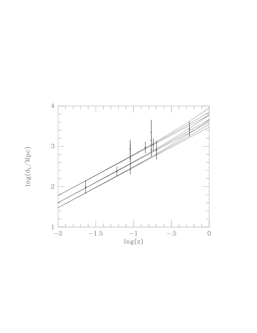
Figure 25: A Hubble diagram based on the distances measured for the nine clusters Abell 1656, 2256, 478, 2142, 1413, 2163, 2218, and 665 and CL 0016+16 (Herbig et al. 1995; Myers et al. 1997; Grainge 1996; Holzapfel et al. 1997a; McHardy et al. 1990; Birkinshaw & Hughes 1994; Jones 1995; Birkinshaw et al. 1991; and Hughes & Birkinshaw 1996). Three values are shown for the distance of Abell 2218 (from Birkinshaw & Hughes, Jones, and McHardy et al.). The Hubble relation is drawn for $H_{0}=50$, $75$, and $100\ {\rm km\,s^{-1}\,Mpc^{-1}}$, with $q_{0}=0$, $1\over 2$, and $1$. The current best fit is for a Hubble constant of about $60\ {\rm km\,s^{-1}\,Mpc^{-1}}$, with no strong constraint on $q_{0}$, but no convincing error can be given because the distance estimates contain correlated systematic errors arising from the calibrations used (see text).

Values of the Hubble constant based on this distance estimation technique are now available for nine clusters. For the clusters with Sunyaev-Zel’dovich effects shown in Fig. 17, 19, 22 and 23, a detailed discussion of the fitting procedures used is given by Birkinshaw et al. (1991), Birkinshaw & Hughes (1994), Jones (1995), Holzapfel et al. (1997a), and Hughes & Birkinshaw (1998). The distances estimated for all nine clusters are displayed as luminosity distances as a function of redshift in Fig. 25. The error bars on the distance estimates are symmetrized errors taken from the individual papers and include systematic errors as well as random errors from uncertainties in the data.

If the results in Fig. 25 are taken at face value, the measurements suggest a Hubble constant near $60\ {\rm km\,s^{-1}\,Mpc^{-1}}$, and have a scatter of about $\pm 20\ {\rm km\,s^{-1}\,Mpc^{-1}}$ (see the similar analysis of Furuzawa 1996). However, we cannot use this to conclude that $H_{0}=60\pm 10\ {\rm km\,s^{-1}\,Mpc^{-1}}$, as seems reasonable based on nine measurements, since those measurements are not truly independent. In particular, only three different telescopes were used in the measurement of $N_{\rm SZ}$ and only two in the measurement of $N_{\rm X}$, so that there are only about two independent X-ray calibrations and three independent Sunyaev-Zel’dovich effect calibrations in the set of results for $H_{0}$. An improvement in the precision of the determination of $H_{0}$, even in the absence of any other problems, must depend on convincing absolute calibrations of the Sunyaev-Zel’dovich effect and X-ray data.

There are a number of other systematic problems in using this technique. The most serious may be a selection effect, which causes the value of $H_{0}$ to be biased low. If the model (118) for $f_{n}$ is modified to make the cluster atmosphere prolate or oblate, then the apparent X-ray and Sunyaev-Zel’dovich effect images of a cluster will be ellipsoidal, or circular if the symmetry axis lies along the line of sight. In the latter case it is clear that it will not be possible to tell that the cluster is aspherical based on the images: indeed, if the core radius of the gas distribution on the line of sight is larger by a factor $Z$ than the core radii in the other two directions, then the density form factor becomes

$$f_{n}=\left(1+{\theta^{2}+(\zeta^{2}/Z^{2})\over{\theta_{\rm c}}^{2}}\right)^{\!-{3\over 2}\beta}\quad.$$ (121)

and the expressions for $\Theta^{(1)}$ and $\Theta^{(2)}$ (119 and 120) remain valid, while the normalizations $N_{\rm X}$ and $N_{\rm SZ}$ both increase by a factor $Z$. The result is that a prolate gas distribution, with the symmetry axis along the line of sight, tends to give a higher central surface brightness than other gas distributions in which the same mass of gas is distributed spherically or with the symmetry axis perpendicular to the line of sight. This causes clusters elongated along the line of sight to be easier to detect in the X-ray or in the Sunyaev-Zel’dovich effect. Such clusters also give biased estimates of distance, since the true angular diameter distance is

$$D_{\rm A}({\rm true})={D_{\rm A}({\rm estimated})\over Z}$$ (122)

if the distance is estimated using (117) not knowing that the cluster is elongated on the line of sight.

An indication of the importance of this effect is shown in Fig. 26, where the estimated value for the Hubble constant from CL 0016+16 is shown as a function of the intrinsic ellipticity (axial ratio) of an ellipsoidal model for the gas distribution. An ellipsoidal model is clearly preferred because of the non-circular X-ray and Sunyaev-Zel’dovich effect isophotes (Figs. 2, 23). The value of the Hubble constant derived by fitting the cluster by a spherical isothermal model is $68\ {\rm km\,s^{-1}\,Mpc^{-1}}$: it can be seen from the figure that by allowing ellipsoidal models with axial ratios as large as 2:1, values over the range $40-100\ {\rm km\,s^{-1}\,Mpc^{-1}}$ can be obtained.

In order to avoid the selection bias in favor of clusters which are elongated along the line of sight, and hence of high surface brightness, and for which low estimates of the Hubble constant are produced, this technique must be applied to a sample of clusters selected without regard to their central surface brightness — perhaps clusters with total X-ray luminosities or flux densities above some limiting value. Such a selection is now possible using the high-sensitivity survey data recently returned by ROSAT (e.g., Ebeling et al. 1996). A corollary is that clusters which are intrinsically hard to study in the X-ray or the Sunyaev-Zel’dovich effect (and including Sunyaev-Zel’dovich effect non-detections) must be included in the set used to measure $H_{0}$: the clusters with the weakest Sunyaev-Zel’dovich effects for their measured X-ray brightnesses are exactly those which imply larger values of $H_{0}$ (albeit with larger observational errors). By contrast, the clusters in Fig. 25 were often selected based on having particularly strong Sunyaev-Zel’dovich effects, and are therefore likely to show an orientation bias. The size of this bias is not known at present, but is probably less than 30 per cent based on the distribution of X-ray axial ratios seen in other cluster samples.

In addition to this bias, there is a further contribution to the error in the estimated distance from the unknown intrinsic shape of cluster atmospheres. The range of observed shapes suggests an error of order 20 per cent is possible (Hughes & Birkinshaw 1998), and calculations of the evolution of cluster atmospheres confirm that this error estimate is reasonable (Roettiger, Stone & Mushotzky 1997; Yoshikawa, Itoh & Suto 1998).

A major component of the error in the estimates of the normalizations often arises from uncertainties in the parameters of the model (equation 121 or some more complicated function). This is particularly evident when the fits are based on older X-ray data (as, for example, Birkinshaw & Hughes 1994). The more recent X-ray imaging data from ROSAT substantially reduce the allowable range of parameters $\beta$ and ${\theta_{\rm c}}$, so that this component of the error in the Hubble constant may be reduced. However, there is an intrinsic uncertainty in the types of gas model that are chosen to describe the atmosphere, and the extent to which they fail to represent aspects of the density and thermal structure of the gas that affect the distance estimate.

Modeling the gas appropriately is important because it is not the same gas that is responsible for the X-ray and Sunyaev-Zel’dovich effect signals that are used to determine the distance. The X-ray surface brightness is dominated by the densest parts of the cluster, since the X-ray emissivity of the gas is proportional to $n_{\rm e}^{2}T_{\rm e}^{1/2}$, while the Sunyaev-Zel’dovich effect is dominated by the lower-density and hotter parts of the gas where the path lengths are longest. This effect is particularly important where single-dish measurements of the Sunyaev-Zel’dovich effect are used, while interferometer maps tend to resolve out structures on the largest angular scales. Uncertainties in the relationship between the contributions of low and high-density regions to the X-ray surface brightness and the Sunyaev-Zel’dovich effect can be avoided by making deep X-ray images, which trace the gas to sufficiently large radii that 90 or 95 per cent of the gas responsible for the Sunyaev-Zel’dovich effect is included. This means, however, tracing the cluster X-ray emission out to at least 10 core radii, at which the surface brightness has fallen to less than $10^{-3}$ of its central value, which often requires long integration times and careful treatment of the background in the X-ray detectors.

Thermal structure in the cluster atmosphere is harder to measure, and to achieve good accuracy in the distance estimates it is necessary to know about the temperature of the cluster gas out to 10 core radii. This is difficult, not only because of the low surface brightnesses of clusters at such radii, but also because of the lower angular resolution of X-ray detectors with useful spectral response. There is little clear information on the changes in temperature of cluster gas as a function of radius outside a few core radii, and an isothermal model (or sometimes a temperature model based on a bright nearby cluster, such as Coma; equation 73) are usually assumed. Systematic errors at the ten per cent level are likely from this uncertainty, and larger errors are possible for more extreme temperature profiles — hydrodynamical models of the evolution of cluster atmospheres (Roettiger et al. 1997; Yoshikawa et al. 1998) suggest that systematic errors of as much as 30 per cent and random errors of order 10 per cent in the Hubble constant may arise because of departures from isothermality.

A different type of density and temperature structure is often found in the central parts of clusters, where the high X-ray emissivity causes the cooling time of the gas to be short. The consequent decrease in central pressure causes a “cooling flow” to be established, with a slow inward drift of the atmosphere, an increase in the central X-ray surface brightness, and a decrease in the central gas temperature (e.g., Fabian et al. 1984). Since the central region in which there is a large change of gas properties is fairly small, it is still possible to use a model of the form (118) to describe the gas distribution, provided that the central X-ray brightness spike is excluded from the X-ray fit, and a corresponding change is made to the fitting for the Sunyaev-Zel’dovich effect. The Sunyaev-Zel’dovich effect will show less modification than the X-ray surface brightness in the presence of a cooling flow because the path length through the cooling region is relatively small, and there is only a small change of electron pressure in that region. However, the cooling gas may partly “fill in” the cm-wave microwave background diminution with free-free emission (Schlickeiser 1991), so that excluding the central region of a cluster from the fit may be important.

Even smaller-scale structure in cluster atmospheres can have an effect on the derived distance. If the intracluster gas is isothermal, but shows density clumping on a scale less than the resolution of the images, then the X-ray emissivity of a small element of gas is enhanced by a factor

$$C_{\rm n}={\langle n_{\rm e}^{2}\rangle\over\langle n_{\rm e}\rangle^{2}}$$ (123)

while the value of $\langle n_{\rm e}\rangle$ is unchanged. Thus the cluster generates more X-ray emission than would be expected based on a uniform atmosphere, and hence the true angular diameter distance is

$$D_{\rm A}({\rm true})=C_{\rm n}\,D_{\rm A}({\rm estimated})$$ (124)

so that with $C_{\rm n}>1$, the true value of the Hubble constant is smaller than the value estimated based on (117) without knowledge of the small-scale clumping.

Unlike the orientation bias, where averaging over a large number of clusters in random orientations with a known distribution of cluster shapes can correct the distance estimate, all cluster atmospheres are expected to be clumpy to some degree, and it is necessary to estimate the value of the clumping in the “average” cluster atmosphere, or to measure it in each cluster, in order to be sure that the distance estimate is not seriously in error. A theoretical estimate of the degree of clumping of the intracluster medium would be difficult, since it must take into account the processes that cause clumping (such as gas injection from the galaxies and energy input from galaxy motions) and that erase clumping (thermal conduction, gas-dynamical processes, and so on). If the clumping is strong and non-isothermal, then detailed X-ray spectroscopy may be able to measure the distribution of temperatures within a cluster, but it is unlikely that full account could be taken of a distribution of $C_{\rm n}$ (with an associated form factor, $f_{C}$) over the cluster volume, nor that the full range of types of clumping could be tested in this way. At present it appears that the clumping of the intracluster medium is relatively weak, since if $C_{\rm n}$ is often large, then it would be expected to show significant variation from cluster to cluster, and the Hubble diagram (Fig. 25) would show stronger scatter than it does. However, the errors on the distance estimates in Fig. 25 at present cannot exclude values of $C_{\rm n}\sim 1.5$, with consequent large systematic error in $H_{0}$.

A variety of other potential problems with this method can be imagined. The Sunyaev-Zel’dovich effect signal could be contaminated by a background primordial anisotropy in the microwave background radiation (e.g., Cen 1998), or by the non-thermal Sunyaev-Zel’dovich effect of a cluster radio halo source, or by the kinematic Sunyaev-Zel’dovich effect, or by diffuse radio emission from cool gas (perhaps clumped into a population of spiral galaxies) towards the edge of the cluster. The X-ray signal could also be contaminated, perhaps by the inverse-Compton emission of relativistic electrons in the cluster radio halo source. Some of these effects are one-sided biases in the distance estimate, others would increase scatter in the Hubble diagram, but in general they should provide additional errors at the level of 10 per cent or less in the distance estimate (Birkinshaw et al. 1991; Holzapfel et al. 1997a).

The potential of this method for measuring the Hubble constant is only now starting to be realized, as better Sunyaev-Zel’dovich effect data become available. I expect a large increase in the number of clusters on a future Hubble diagram like Fig. 25, and that useful cosmological results will be obtained, especially as the maximum redshift at which an Sunyaev-Zel’dovich effect cluster is detected increases above $0.55$. However, in view of the likely presence of residual systematic effects in the data and the low accuracy of any one measurement, I believe that it is premature to use them to estimate the values of the deceleration parameter and cosmological constant, as has been attempted recently by Kobayashi, Sasaki & Suto (1996).

11.2 Contributions to the CMBR spectrum

The cosmological effects of the Sunyaev-Zel’dovich effect fall into two categories: the integrated effect on the spectrum (discussed in this section) and the angular fluctuation pattern that is created (Sec. 11.3). Both the gas in clusters of galaxies and the distributed hot intergalactic medium between clusters will contribute to these effects: indeed, at a general level we can consider the cluster gas to be merely a strongly clumped fraction of the hot intergalactic medium. The cosmological Sunyaev-Zel’dovich effects then measure the projected electron pressure distribution since recombination.

It is convenient in discussing the effect of the intergalactic medium (IGM) on the CMBR to work in terms of the fraction of the critical density that this gas comprises. This is described by the quantity

$$\Omega_{\rm IGM}={\rho_{\rm IGM}\over\rho_{\rm crit}}$$ (125)

where the critical density, $\rho_{\rm crit}$ (equation 2) just closes the Universe. Limits to the contribution of neutral gas to $\Omega_{\rm IGM}$ are already stringent, because of the absence of neutral hydrogen absorption features in the spectra of high-redshift quasars (the Gunn-Peterson test; Gunn & Peterson 1965), with a recent limit on the optical depth $\tau_{\rm GP}<0.07$ at redshifts near 4.3 based on a spectrum of a quasar at $z=4.7$ (Giallongo et al. 1994). Further limits on the contribution of hot gas to $\Omega_{\rm IGM}$ can be set based on the X-ray background, most of which can be accounted for by the integrated emission of active galaxies and quasars (Comastri et al. 1995). At low energies it has been suggested that the bremsstrahlung of hot gas in clusters and groups of galaxies may make a significant contribution to the X-ray background, or even over-produce the background under some models for cluster evolution (Burg et al. 1993), while the possibility that a diffuse intergalactic medium is responsible for much of the X-ray background was suggested by Field & Perrenod (1977).

If some significant contribution to the X-ray background does come from distributed gas, then the assumption that the gas is fully ionized out to some redshift $z_{\rm ri}$ (at time $t_{\rm ri}$) leads to an optical depth for inverse-Compton scatterings between ourselves and the epoch of recombination of

$$\tau_{\rm e} = \int_{t_{\rm ri}}^{t_{\rm 0}}\,\sigma_{\rm T}\,n_{\rm e}(z)\,c\,dt$$ (126)

$$= {c\sigma_{\rm T}n_{\rm e0}\over H_{0}}\,\int_{0}^{z_{\rm ri}}\,dz{(1+z)\over(1+\Omega_{0}z)^{1/2}}$$

where $n_{\rm e0}$ is the electron density today and I have assumed a Friedmann-Robertson-Walker cosmology with zero cosmological constant. If the thermal history of this intergalactic plasma is parameterized by a redshift-dependent electron temperature, $T_{\rm e}(z)$, then the Comptonization parameter is

$$y = \int_{t_{\rm ri}}^{t_{\rm 0}}\,\sigma_{\rm T}\,n_{\rm e}(z)\,c\,{{k_{\rm B}}T_{\rm e}(z)\over m_{\rm e}c^{2}}\,dt$$ (127)

$$= {c\sigma_{\rm T}n_{\rm e0}\over H_{0}}\,{{k_{\rm B}}\over m_{\rm e}c^{2}}\int_{0}^{z_{\rm ri}}\,dz\,T_{\rm e}(z)\,{(1+z)\over(1+\Omega_{0}z)^{1/2}}.$$

For re-ionization redshifts $\lesssim 30$, and any $\Omega_{0}<1$, the scattering optical depth is less than about $2.6\,\Omega_{\rm IGM}\,h_{\rm 100}$, and when the integral in (127) is performed for plausible thermal histories of the intergalactic medium (e.g., Taylor & Wright 1989; Wright et al. 1996), then the recent COBE FIRAS limit $y<15\times 10^{-6}$ (Fixsen et al. 1996) leads to a limit on the electron scattering optical depth (averaged over the sky) of less than $3\times 10^{-4}$ (Wright et al. 1994). This corresponds to an electron density that is $\approx 100$ times less than the density needed to produce a significant fraction of the X-ray background by thermal bremsstrahlung, which in turn suggests that a uniform, hot, IGM produces less than $10^{-4}$ of the X-ray background, and that a significant fraction of the X-ray background can only arise from thermal bremsstrahlung if the gas has a filling factor $<10^{-4}$ on the sky.

Direct calculations of the effects of clusters of galaxies on the spectrum of the CMBR have been made by Markevitch et al. (1991) and Cavaliere, Menci & Setti (1991). An integration like that in (127) must now be performed over an evolving population of clusters of galaxies, with varying space density, size, gas properties, etc. Markevitch et al. used self-similar models for the variations of cluster properties with redshift. These models are characterized by a power-law index $n$, which defines the relationship between the redshift and density, size, mass, and comoving number density scales of a population of clusters. Specifically, the mass scale of the population is

$$M^{\ast}\propto(1+z)^{-6/(n+3)}$$ (128)

if $\Omega_{0}=1$ and a more complicated expression for other values of $\Omega_{0}$ (White & Rees 1978; Kaiser 1986). For the physical range $-3<n<1$, slower evolution of $M^{\ast}$ is obtained for larger values of $n$.

Markevitch et al. (1991) normalized the properties of a population of clusters using present-day observed density, temperature, and structure based on X-ray data, and integrated over this population as it evolved to calculate the mean Comptonization parameter that would result. The important parameters of this calculation are $n$, $\Omega_{0}$, and $z_{\rm max}$, the maximum redshift for which clusters can be said to follow the evolution model (128). Using the most recent limits on the Comptonization parameter from the analysis of the COBE FIRAS data (Fixsen et al. 1996), the numerical results obtained by Markevitch et al. can be interpreted as implying that $z_{\rm max}\lesssim 10$ for a non-evolving cluster population, and that $\Omega_{0}\gtrsim 0.1$ if the cluster population evolves with $-1\leq n\leq 1$. Similar conclusions can be drawn from the results given by Cavaliere et al. (1991).

The closeness of the COBE FIRAS limit to the Comptonization parameter to the prediction from these models for the change of cluster properties with redshift indicates the power of the FIRAS data in constraining models for the evolution of clusters, and perhaps the value of $\Omega_{0}$ (Markevitch et al. 1991; Wright et al. 1994). It should now be possible to take into account all the constraints on the population of clusters containing dense atmospheres, including the controversial “negative evolution” of the population of X-ray clusters (Edge et al. 1990; Gioia et al. 1990a), to place strong restrictions on the range of acceptable models of cluster evolution.

11.3 Fluctuations in the CMBR

The Sunyaev-Zel’dovich effect not only causes changes in the integrated spectrum of the CMBR, but also induces fluctuations in its brightness which appear superimposed on the fluctuations arising from the formation of structure in the early Universe (Sec. 1.3). The angular scale of these new structures in the CMBR will depend on their origin, and on the large-scale structure of the Universe. Constraints on both the manner in which clusters evolve and $\Omega_{0}$ have been obtained by the limits to the fluctuation power from arcminute-scale experiments.

The present review concentrates on the fluctuations induced in the CMBR by clusters and superclusters of galaxies, but a diffuse ionized intergalactic medium with density and velocity irregularities, such as those created as large-scale structure develops, will also produce significant CMBR fluctuations. The best-known of these is the Vishniac effect (Vishniac 1987), which is due to the kinematic Sunyaev-Zel’dovich effect of a perturbation in the electron density in the (re-ionized) diffuse intergalactic medium. Discussions of this, and other, structures that are superimposed on the primordial spectrum by inhomogeneities in the re-ionized intergalactic medium are given by Dodelson & Jubas (1995) for $\Omega_{0}=1$, by Persi (1995) for open Universes, and in the review of White et al. (1994).

Cluster Sunyaev-Zel’dovich effects can have a strong influence on the CMBR because, unlike “normal” astrophysical sources, the surface brightness of the Sunyaev-Zel’dovich effect from a cluster is independent of redshift, and does not suffer $(1+z)^{-4}$ fading. This is because the effect is a fractional change in the brightness of the CMBR, and the CMBR’s energy density itself increases with redshift as $(1+z)^{4}$, cancelling out the dimming effect of cosmology. The integrated flux density of a cluster at observed frequency $\nu$,

$$S_{\nu}=j(x)\int d\Omega\int{{k_{\rm B}}{T_{\rm e}}\over m_{\rm e}c^{2}}\,\sigma_{\rm T}\,n_{\rm e}\,dl$$ (129)

in the Kompaneets approximation, where $j(x)$ is the Kompaneets spectral function (defined by $\Delta n=yj(x)$ in equation 59), $x={h\nu/{k_{\rm B}}{T_{\rm rad}}}$ is the usual dimensionless frequency, and the first integral is over the solid angle of the cluster. Equation (129) can be written as an integral over the cluster volume

$$S_{\nu}=j(x)\int d^{3}x\,{{k_{\rm B}}{T_{\rm e}}\over m_{\rm e}c^{2}}\,{\sigma_{\rm T}\,n_{\rm e}\over d_{A}^{2}}$$ (130)

which for a constant electron temperature over the cluster can be written simply in terms of the total number of electrons in the cluster, $N_{\rm e}$, and the angular diameter and luminosity distances, $D_{\rm A}$ and $D_{\rm L}$, as

$$S_{\nu}=j(x)\,{{k_{\rm B}}{T_{\rm e}}\over m_{\rm e}c^{2}}\,{\sigma_{\rm T}\,N_{\rm e}\over D_{\rm A}^{2}}=j(x)\,{{k_{\rm B}}{T_{\rm e}}\over m_{\rm e}c^{2}}\,\sigma_{\rm T}\,N_{\rm e}\,{(1+z)^{4}\over D_{L}^{2}}\quad.$$ (131)

This indicates that the cluster’s apparent luminosity increases as $(1+z)^{4}$ — or, alternatively, that its flux density is a function of intrinsic properties and angular diameter distance only.

As a result, a population of clusters with the same $N_{\rm e}$ and $T_{\rm e}$, observed at different redshifts, will exhibit a minimum flux density at the redshift of maximum angular diameter distance in that cosmology (Korolyev, Sunyaev & Yakubtsev 1986). Although this might provide a cosmological test for $\Omega_{0}$, in practice clusters exhibit a wide range of properties and change significantly with redshift so it might be difficult to distinguish the effects of cosmology, cluster populations, and cluster evolution. The realizable cluster source counts (the histogram of sky brightnesses observed by a particular telescope of given properties) will then depend on a complicated mix of observational characteristics of the telescope used, the cosmological parameters, and the evolution of the cluster atmospheres. Nevertheless, Markevitch et al. (1994) suggest that a study of source counts at the ${\rm\mu Jy}$ level (at cm-wavelengths) or at the ${\rm mJy}$ level (at mm-wavelengths) can constrain the spectrum of cluster masses (which determines the value of $y$), the cosmological parameter $\Omega_{0}$, and the redshift of cluster formation. Using the results of arcminute-scale measurements of the anisotropy in the CMBR (the OVRO RING experiment; Myers 1990, Myers et al. 1993), Markevitch et al. were able to rule out slowly-evolving ($n=1$ in eq. 128) models in an open Universe with $\Omega_{0}<0.3$.

More detailed treatments of the effects of foreground clusters on the CMBR express their results in the formalism of Sec. 1.3 that is used to describe primordial fluctuations. A number of different assumptions about the cosmology and evolution of large scale structure have been used to calculate the amplitude and angular pattern of the foreground fluctuations (Rephaeli 1981; Cavaliere et al. 1986; Cole & Kaiser 1988; Schaeffer & Silk 1988; Thomas & Carlberg 1989; Markevitch et al. 1992; Makino & Suto 1993; Bartlett & Silk 1994a, 1994b; Ceballos & Barcons 1994; Colafrancesco et al. 1994; see also the review by Rephaeli 1995b). A uniform result of the calculations is that the distribution of sky brightness fluctuations that result is strongly non-Gaussian and asymmetrical since it is composed of negative or positive sources (depending on the frequency of observation, and the sign of $j(x)$) with varying numbers of sources on any line of sight or contained in a particular telescope beam (e.g., Markevitch et al. 1992). However, the amplitude and angular scale of the cluster-generated fluctuations depend strongly on the pattern of cluster evolution and the cosmology assumed. If the negative evolution of cluster atmospheres is strong (negative $n$ in the self-similar model used by Markevitch et al.; eq. 128), then the distribution will be dominated by low-redshift clusters and the value of $\Omega_{0}$ will not be important. For slow evolution or no evolution, the value of $\Omega_{0}$ becomes important, since the variation of $D_{\rm A}$ with redshift dictates the appearance of the microwave background sky.

The angular pattern of fluctuations that results generally shows significant power in the two-point correlation function (eq. 8) at the level $10^{-6}\lesssim\langle\Delta T/T\rangle\lesssim 10^{-5}$ on sub-degree scales (e.g., Colafrancesco et al. 1994), but some models for the evolution of clusters (and cluster atmospheres) can be ruled out from the absence of large anisotropies in the OVRO data of Readhead et al. (1989), Myers et al. (1993), or other experiments, and some cosmological parameters can be excluded under particular models for the evolution of cluster atmospheres. Since different models can make quite different predictions for the angular pattern and the amplitude of fluctuations, there is a potential for studying the processes that lead to the accumulation of cluster atmospheres through a study of the microwave background radiation on the range of angular scales (arcminute to degree) on which the cluster signal should be significant.

If the evolution of clusters is to be studied in this way, then observations of the cluster-induced Sunyaev-Zel’dovich fluctuation pattern would need to be made over a wide range of angular scales in order to validate or falsify any one of the models unambiguously. This range of angular scales overlaps that occupied by the stronger “Doppler peaks” in the primordial spectrum of fluctuations, so that the cluster signal may be hard to detect (see, e.g., the review of Bond 1995). The cluster signal is also an important contaminant of the Doppler peaks, which are expected to be a useful cosmological indicator and whose characterization is an important aim of the coming generation of CMBR satellites (MAP and Planck). Fortunately, measurements of the anisotropy pattern at several frequencies can be used to separate Sunyaev-Zel’dovich effects imposed by clusters and the primordial fluctuation background (Rephaeli 1981): the sensitivity required to achieve clean separations is formidable, but achievable with the current baseline design of the satellites’ detectors.

An illustration of these results is given in Fig. 27, which shows the relative strengths of the power spectra of primordial fluctuations, the thermal and kinematic Sunyaev-Zel’dovich effects, and the moving-cluster Rees-Sciama effect in a $\Lambda$-CDM cosmology (involving a significant cosmological constant and cold dark matter) with an evolving cluster population (Molnar 1998). Although the details of the power spectra depend on the choice of cosmology and the physics of cluster evolution (compare, e.g., Aghanim et al. 1998), the general features are similar in all cases. For $l\mathrel{\hbox{\raise 2.15277pt\hbox{$<$}\hbox to0.0pt{\hss\lower 2.15277pt\hbox{$\sim$}}}}3000$, the power spectrum is dominated by the signal from primordial structures. The kinematic Sunyaev-Zel’dovich and Rees-Sciama effects from the cluster population are a factor $\mathrel{\hbox{\raise 2.15277pt\hbox{$>$}\hbox to0.0pt{\hss\lower 2.15277pt\hbox{$\sim$}}}}10^{2}$ less important than the thermal Sunyaev-Zel’dovich effect. Thus the evident detectability of the thermal Sunyaev-Zel’dovich effect (Sec. 9) is principally due to its strongly non-gaussian nature and its association with clusters known from optical or X-ray observations, and not to its intrinsic power. Future work, for example the all-sky surveys that MAP and Planck will perform, will have the spectral discrimination to detect the thermal Sunyaev-Zel’dovich effect on a statistical basis, and should measure the power spectra of the thermal Sunyaev-Zel’dovich effect on small angular scales ($l\mathrel{\hbox{\raise 2.15277pt\hbox{$>$}\hbox to0.0pt{\hss\lower 2.15277pt\hbox{$\sim$}}}}300$; Aghanim et al. 1997; Molnar 1998).

The sensitivity of the Sunyaev-Zel’dovich effect power spectrum to cosmology is illustrated in Fig. 28 (Molnar 1998). Variations of a factor $>10$ in the power of fluctuations induced by the thermal Sunyaev-Zel’dovich effect are evident at $l>300$: although this might be used as a cosmological test, the locations and strengths of the Doppler peaks in the primordial anisotropy power spectrum are more powerful. However, the amplitude of the Sunyaev-Zel’dovich effect power spectrum depends on how clusters evolve, and measurements of this power spectrum over a wide range of $l$ should provide an important test of models of the formation of structure in the Universe.

Superclusters of galaxies, and the gas pancakes from which superclusters may have formed, are expected to make only a minor contributions to the fluctuation spectrum (Rephaeli 1993; SubbaRao et al. 1994). Once again, the angular scales on which the supercluster signals appear are similar to those of the Doppler peaks, and both good frequency and angular coverage will be needed to distinguish the primordial and foreground signals.

11.4 Quasars and the Sunyaev-Zel’dovich effects

The intergalactic medium near a quasar must be strongly ionized by the quasar’s radiation. These hot gas bubbles are likely to be overpressured, and to expand into their surrounding intergalactic medium. Thus both thermal and kinematic Sunyaev-Zel’dovich effects may arise near quasars, and we might expect a contribution from quasars in the spectrum of fluctuations in the CMBR (Aghanim et al. 1996). Aghanim et al. find that the kinematic effect dominates, and can cause local changes of $\approx 300\ {\rm\mu K}$ in the brightness temperature of the CMBR on scales up to $\approx 1$ deg. Whether such structures are indeed present in the CMBR will be tested by the next generation of CMBR surveys.

Sunyaev-Zel’dovich effects may also be seen from the Lyman $\alpha$ absorption clouds seen in quasar spectra (Loeb 1996). The expected effects are much smaller, typically only a few ${\rm\mu K}$ and with angular sizes of less than an arcminute, from the varying numbers of Ly$\alpha$ systems on different lines of sight. Here again the dominant contribution to the signal is from the kinematic Sunyaev-Zel’dovich effect, and relies on large velocities acquired by the Ly$\alpha$ absorbing clouds as large-scale structure forms.

Either of these effects, or possibly a Sunyaev-Zel’dovich effect from a quasar-related cluster with a deficiency of bright galaxies, or a kinematic effect from colliding QSO winds (Natarajan & Sigurdsson 1997), might explain the observations of CMBR anisotropies towards the quasars PHL 957 (Andernach et al. 1986) and PC 1643+4631 (Jones et al. 1997). However, the reality of these detections remains in some dispute until they are independently confirmed.

12 Continuing research and the future of the Sunyaev-Zel’dovich effect

Developments in the technologies of microwave background observation are continuing, so that there is every reason to expect that all clusters of galaxies with luminous X-ray emitting atmospheres will eventually be detected in their Sunyaev-Zel’dovich effects. Cm-wave measurements, with traditional single-dish telescopes and radiometers, are unlikely to be as effective, in the long run, as mm-wave measurements using bolometers simply because many strong X-ray clusters also contain bright radio sources whose extended emission will not easily be avoided at cm wavelengths. Nevertheless, radiometric surveys will be increasingly good at locating Sunyaev-Zel’dovich effects as arrays of receivers become more common and the bandwidths and noise temperatures of radiometers continue to improve. Over the next few years I expect the most spectacular improvements in type of Sunyaev-Zel’dovich effect work to emerge from spectral measurements of the Sunyaev-Zel’dovich effects (with the principal aim of setting limits to the velocities of clusters of galaxies) and from interferometric mapping of clusters, and indeed of the CMBR itself, using optimized interferometers.

A possible design for such an optimized array, tuned for work on clusters at redshifts $\gtrsim 0.1$, would provide ${\rm\mu K}$ sensitivity, a full-resolution synthesized beam $\approx 30$ arcsec, and good sensitivity to angular scales $\gtrsim 5$ arcmin. For operation at cm wavelengths, this requires antennas of 10 m diameter or less, baselines from 10-100 m, and sufficient antennas simultaneously present that high sensitivity is attained rapidly and so that radio source contamination can be well mapped. Such a system is similar to BIMA or the OVMMA operated at cm-wavelengths, as done by Carlstrom et al. (1996) and Patel et al. (1997), or to the planned VSA and CBI instruments. Alternatively, smaller antennas and baselines (and smaller fractional bandwidths) could be used at a wavelength of 3 mm with a dedicated microwave background mapping array. This would have the advantages of better rejection of signals from radio sources, and more leverage on the spectrum of the Sunyaev-Zel’dovich effects with moderate changes in operating frequency, but would need a good site if it is to operate efficiently.

Survey work, as is presently carried out from ground-based antennas, could be done more efficiently from satellite systems, but with a large cost. A good initial aim for a major survey would be to provide $10\ {\rm\mu K}$ or better sensitivity on a large set of clusters selected without orientation bias, and hence suitable for statistical interpretation of the Sunyaev-Zel’dovich effects for cluster properties and cosmological parameters. Many clusters are likely to be detected in such an unbiased fashion in the all-sky CMBR surveys that will be produced by the next generation of mapping satellites (MAP and Planck). Long-duration balloon projects (such as SOAR) should also be able to produce excellent surveys of clusters. Cross-correlation studies between CMBR maps of large fractions of the sky and cluster (extended) X-ray sources from the ROSAT survey should give good indications of the distribution of cluster properties.

It is likely to be space-based or balloon-based operation of bolometer arrays that will produce the best measurements of Sunyaev-Zel’dovich effect spectra of clusters and hence should measure the peculiar velocities of clusters (or at least the peculiar velocities of cluster gas, which might not be the same in all cases). Combined structural and spectral measurements of a cluster, coupled with X-ray spectral and mapping information, should allow the effects of primordial structure contamination of the velocity signal in the CMBR to be minimized, since it is unlikely that the primordial perturbations behind a cluster will be distributed with an angular structure that is a close match to the cluster’s gas distribution. The use of a matched filter based on the X-ray data may not be effective in all cases, however, if the structure of cluster atmospheres is found to be complicated by density and temperature inhomogeneities (as is particularly likely at higher redshifts).

Obtaining these Sunyaev-Zel’dovich effect data at high signal/noise will not be useful without matching high-quality X-ray data. Fortunately, such X-ray data will be available shortly. We are already obtaining large samples of clusters of galaxies from ROSAT (Ebeling et al. 1996), and with AXAF we will be able to obtain detailed (arcsec-resolution) X-ray images of these clusters and spatially-resolved X-ray spectra. Sunyaev-Zel’dovich interferometric maps would then be a powerful indicator of structural inhomogeneities in the gas or anomalous heating (e.g., regions of clumping, perhaps in galaxy wakes). Sunyaev-Zel’dovich and X-ray data together should provide good distance measurements over a wide range of redshifts, leading to a substantial increase in the number of clusters in the Hubble diagram (Fig. 25), but the estimation of reliable Hubble constant and deceleration parameter demands an improvement in the level of systematic errors in that diagram, especially through improvements in the calibration of the Sunyaev-Zel’dovich effect data (i.e., much better absolute calibrations of the planets, and better transfer of these calibrations to secondary sources) and the X-ray detectors.

Other CMBR data on clusters of galaxies may also become available soon. The detection of the kinematic Sunyaev-Zel’dovich effect and the Rees-Sciama effects from the transverse motions of clusters of galaxies would provide a full three-dimensional velocity field of clusters, allowing the study of the evolution of this velocity field with redshift, and providing fundamental constraints on the physics of galaxy clustering. Observations of Sunyaev-Zel’dovich and other effects from clusters of galaxies (or the puzzling cluster-like structures in regions of blank sky) are likely to provide much powerful information for cosmology and studies of clusters over the next decade or two.

Figure 1: The spectrum of the microwave background radiation, and the microwave background radiation after passage through an (exaggerated) scattering atmosphere with $y=0.1$ and $\tau\beta=0.05$ (as defined in Sections 3 and 6), compared with the integrated emission from the bright radio source Cygnus A as observed by a telescope with solid angle $\Omega_{\rm beam}=1$ square deg. Note that the microwave background radiation dominates at high frequencies. Scattering (the Sunyaev-Zel’dovich effect) causes a fractional decrease in the low-frequency intensity of the CMBR that is proportional to $y$. The location of the cross-over point, where the scattered CMBR and the unscattered CMBR have equal brightness, is a measure of $\tau\beta$. This scattered spectrum was calculated using the Kompaneets formula (59), rather than the relativistic results (eq. 51) of Rephaeli (1995a), and hence is only accurate for low cluster gas temperatures (see Sec. 3.3), although the difference is imperceptible in this figure.

Figure 3: The scattering geometry, in the frame of rest of the electron before the interaction. An incoming photon, at angle $\theta$ relative to the $x_{\rm e}$ axis, is deflected by angle $\phi_{12}$, and emerges after the scattering at angle $\theta^{\prime}$ with almost unchanged energy (equation 21). In the observer’s frame, where the electron is moving with velocity $\beta c$ along the $x_{\rm e}$ axis, the photon changes energy by an amount depending on $\beta$ and the angles $\theta$ and $\theta^{\prime}$ (equation 25).

Figure 4: The scattering probability function $P(s;\beta)$, for $\beta=0.01$, $0.02$, $0.05$, $0.10$, $0.20$, and $0.50$. The function becomes increasingly asymmetric and broader as $\beta$ increases.

Figure 5: The scattering kernel, $P_{1}(s)$, for gases at 5.1 keV and 15.3 keV. The solid line shows the scattering kernels calculated according to (33), as derived by Rephaeli (1995a). The dotted line indicates the scattering kernels as calculated by Sunyaev (1980), based on the results of Babuel-Peyrissac & Rouvillois (1969).

Figure 6: The scattering kernel, $P_{1}(s)$, for a power-law electron distribution with energy index $\alpha=2.5$ (see equation 37). The stronger upscattering tail here, relative to Fig. 5, is caused by the higher proportion of fast electrons in distribution (37) than (35).

Figure 7: The spectral deformation caused by inverse-Compton scattering of an incident Planck spectrum after a single scattering from a thermal population of electrons as a function of dimensionless frequency $x=h\nu/{k_{\rm B}}{T_{\rm rad}}=0.0176(\nu/{\rm GHz})$, with scaling $I_{0}={2h\over c^{2}}\left({{k_{\rm B}}{T_{\rm rad}}\over h}\right)^{3}$. Left, for electrons at ${k_{\rm B}}{T_{\rm e}}=5.1$ keV; right for electrons at ${k_{\rm B}}{T_{\rm e}}=15.3$ keV. The result obtained from the Kompaneets kernel is shown as a dotted line. The shape of the distortion is independent of ${T_{\rm e}}$ (and the amplitude is proportional to ${T_{\rm e}}$) for the Kompaneets kernel, but the relativistic expression leads to a more complicated form.

Figure 8: The fractional spectral deformation caused by inverse-Compton scattering of an incident Planck spectrum by a single scattering from a power-law population of electrons with $\alpha=2.5$ (equation 37). The spectral deformation has a similar shape to that seen in Fig. 7, but with a deeper minimum and more extended tail. This arises from the larger frequency shifts caused by the higher Lorentz factors of the electrons (see Fig. 6).

Figure 9: The variation of the positions of the minimum, zero, and maximum of the spectrum of the thermal Sunyaev-Zel’dovich effect, $\Delta I(x)$, as the electron temperature varies. The positions of the spectral features are described by the dimensionless frequency $x=h\nu/{k_{\rm B}}{T_{\rm rad}}$, and the electron temperature is characterized by $\Theta={k_{\rm B}}{T_{\rm e}}/m_{\rm e}c^{2}$.

Figure 10: A model for CL 0016+16 assuming that the cluster is oblate with the symmetry axis in the plane of the sky, and with the structural parameters fixed by fits to the ROSAT PSPC image (Fig. 2). Left: the model X-ray surface brightness. Right: the model Sunyaev-Zel’dovich effect. The contours in both plots are spaced at intervals of 12.5 per cent of the peak effect — note that the Sunyaev-Zel’dovich effect shows a much greater angular extent than the X-ray emission (compare the angular dependences in equations 66 and 67). The central Sunyaev-Zel’dovich effect predicted on the basis of the X-ray data is $-0.84h_{100}^{-1/2}$ mK.

Figure 12: The geometry for the discussion of the kinematic Sunyaev-Zel’dovich effect, as seen in the frame of an observer at rest in the Hubble flow.

Figure 13: A representative beam and position-switching scheme, and background source field: for observations of a point near the center of Abell 665 by the Owens Valley Radio Observatory 40-m telescope. The locations of the on-source beam and reference beams in this symmetrical switching experiment are shown as solid circles. The main beam is first pointed at the center of the cluster with the reference beam to the NW while beam-switched data are accumulated. The position of the main beam is then switched to the SE offset position, with the reference beam pointed at the center of the cluster, and more beam-switched data are accumulated. Finally, the main beam is again pointed at the cluster center. As the observation extends in time, the offset beam locations sweep out arcs about the point being observed, with the location at any one time conveniently described by the parallactic angle, $p$. Since Abell 665 is circumpolar from the Owens Valley, the reference arcs close about the on-source position: however, the density of observations is higher at some parallactic angles because $p$ is not a linear function of time (see equation 91).

Figure 14: The observing efficiency factor, $\eta$, as a function of redshift, for observations of clusters with core radius $300\ {\rm kpc}$ and $\beta=0.67$, using the OVRO 40-m telescope at 20 GHz and assuming $h_{100}=0.5$ and $q_{0}={1\over 2}$. $\eta$ is defined to be the central effect seen by the telescope divided by the true amplitude of the Sunyaev-Zel’dovich effect, and measures the beam-dilution and beam-switching reductions of the cluster signal. The decrease in $\eta$ at $z>0.15$ is slow, so that these observations would be sensitive to the Sunyaev-Zel’dovich effects over a wide redshift range.

Figure 17: Measurements of changes in the apparent brightness temperature of the microwave background radiation as a function of declination near the clusters CL 0016+16, Abell 665 and Abell 2218 (Birkinshaw et al. 1998). The largest Sunyaev-Zel’dovich effect is seen at the point closest to the X-ray center for each cluster (offset from the scan center in the case of Abell 665), and the apparent angular sizes of the effects are consistent with the predictions of simple models based on the X-ray data. The horizontal lines delimit the range of possible zero levels, and the error bars include both random and systematic components.

Figure 19: Sample 4.6-arcmin difference data from the 1994 SuZIE observations of Abell 2163 (Holzapfel et al. 1997a). The upper panel shows data taken across the cluster center together with the best-fitting (non-isothermal) model of the cluster Sunyaev-Zel’dovich effect based on the X-ray data (heavy line) and the same model with $\pm 1\sigma$ errors on the amplitude (upper and lower light lines). The middle panel compares the predictions of the same model with the data taken 2.2 arcmin south of the cluster center, while the bottom panel shows the corresponding model fit to a region of blank sky well separated from the cluster but at a similar declination.

Figure 20: The mm to far-IR spectrum of Abell 2163 (from Lamarre et al. 1998). The solid line shows a best-fit model composed of dust emission and Sunyaev-Zel’dovich effects. The dashed line shows the dust contribution to the overall spectrum. The dash-dotted line shows the Sunyaev-Zel’dovich thermal effect. The insert shows the contribution of the kinematic Sunyaev-Zel’dovich effect in the mm to cm part of the spectrum.

Figure 21: The interferometer response that would be expected from a 6-cm VLA observation of the Sunyaev-Zel’dovich effect from cluster CL 0016+16, normalized to the effect with zero baseline. The minimum separation of VLA antennas is 650 wavelengths, but projection effects mean that the minimum observable baseline is roughly equal to the antenna diameter, or about 420 wavelengths. Thus on the shortest one or two baselines, for a brief interval, the VLA can observe about 25 per cent of the total available Sunyaev-Zel’dovich effect (which corresponds to about $-0.9\ {\rm mJy}$ if the central Sunyaev-Zel’dovich effect is about $-1$ mK). Consequently, the VLA is a poor instrument for observing the Sunyaev-Zel’dovich effect in this cluster.

Figure 24: An image of the Sunyaev-Zel’dovich effect from the cluster MS 0451.6-0305 at $z=0.55$, as measured by Joy et al. (in preparation) using the OVMMA. The beamshape of the image is shown in the lower left corner. This cluster was first detected in the Einstein Medium-Sensitivity Survey (Gioia et al. 1990b), and therefore can be regarded as a part of an X-ray complete sample.

Figure 26: The dependence of the Hughes & Birkinshaw’s (1998) estimate of the value of the Hubble constant on assumptions about the oblateness or prolateness of CL 0016+16 in the extreme case where the cluster symmetry axis lies in the plane of the sky.

Figure 27: The zero-frequency power spectrum of primordial microwave background anisotropies (solid line; calculated using the CMBFAST code of Zaldarriaga et al. 1998), the thermal Sunyaev-Zel’dovich effect (dotted line), the kinematic Sunyaev-Zel’dovich effect (short dashed line), and the Rees-Sciama effect from moving clusters (long dashed line) predicted in the $\Lambda$-CDM cosmology discussed by Bahcall & Fan (1998). Figure from Molnar (1998).

Figure 28: The zero-frequency power spectrum of primordial microwave background anisotropies (solid lines; calculated using the CMBFAST code of Zaldarriaga et al. 1998), and the Sunyaev-Zel’dovich effects of an evolving population of clusters (dotted lines) predicted in three cosmological models consistent with the COBE anisotropies: the open CDM, $\Lambda$-CDM, and “standard” CDM models discussed by Bahcall & Fan (1998). Figure from Molnar (1998).

Table 1: Radiometric measurements of the Sunyaev-Zel’dovich effects

Paper	Technique	$\nu$	$\theta_{\rm h}$	$\theta_{\rm b}$	$\theta_{\rm s}$
		$({\rm GHz})$	$({\rm arcmin})$	$({\rm arcmin})$	$({\rm arcmin})$
Parijskij 1972	DS	7.5	$1.3\times 40$	$\cdots$	290
Gull & Northover 1976	BS+PS	10.6	4.5	15.0	$\cdots$	$\ast$
Lake & Partridge 1977	BS+PS	31.4	3.6	9.0	$\cdots$	$\ast$
Rudnick 1978	BS+DS	15.0	2.2	17.4	60-120
Birkinshaw et al. 1978a	BS+PS	10.6	4.5	15.0	$\cdots$	$\ast$
Birkinshaw et al. 1978b	BS+PS	10.6	4.5	15.0	$\cdots$	$\ast$
Perrenod & Lada 1979	BS+PS	31.4	3.5	8.0	$\cdots$
Schallwich 1979	BS+DS	10.7	1.2	8.2	15	$\ast$
Lake & Partridge 1980	BS+PS	31.4	3.6	9.0	$\cdots$
Birkinshaw et al. 1981a	BS+PS	10.7	3.3	14.4	$\cdots$	$\ast$
Birkinshaw et al. 1981b	BS+PS	10.6	4.5	15.0	$\cdots$
Schallwich 1982	BS+DS	10.7	1.2	8.2	15
Andernach et al. 1983	BS+DS	10.7	1.2	3.2, 8.2	15
Lasenby & Davies 1983	BS+PS	5.0	$8\times 10$	30	$\cdots$
Birkinshaw & Gull 1984	BS+PS	10.7	3.3	20.0	$\cdots$
	BS+PS	10.7	3.3	14.4	$\cdots$
	BS+PS	20.3	1.8	7.2	$\cdots$
Birkinshaw et al. 1984	BS+PS	20.3	1.8	7.2	$\cdots$
Uson & Wilkinson 1984	BS+PS	19.5	1.8	8.0	$\cdots$	$\ast$
Uson 1985	BS+PS	19.5	1.8	8.0	$\cdots$	$\ast$
Andernach et al. 1986	BS+DS	10.7	1.18	3.2, 8.2	15
Birkinshaw 1986	BS+PS	10.7	1.78	7.15	$\cdots$	$\ast$
Birkinshaw & Moffet 1986	BS+PS	10.7	1.78	7.15	$\cdots$	$\ast$
Radford et al. 1986	BS+DS	90	1.3	4.0	10
	BS+PS	90	1.2	4.3	$\cdots$
	BS+PS	105	1.7	19	$\cdots$
Uson 1986	BS+PS	19.5	1.8	8.0	$\cdots$	$\ast$
Uson & Wilkinson 1988	BS+PS	19.5	1.8	8.0	$\cdots$
Birkinshaw 1990	BS+PS	20.3	1.78	7.15	$\cdots$	$\ast$
Klein et al. 1991	BS+DS	24.5	0.65	1.90	6.0
Herbig et al. 1995	BS+PS	32.0	7.35	22.16	$\cdots$
Myers et al. 1997	BS+PS	32.0	7.35	22.16	$\cdots$
Uyaniker et al. 1997	DS	10.6	1.15	$\cdots$	10
Birkinshaw et al. 1998	BS+PS	20.3	1.78	7.15	$\cdots$
Tsuboi et al. 1998	BS+PS	36.0	0.82	6.0	$\cdots$

Note. — The technique codes are BS for beam-switching, PS for position-switching, DS for drift- or driven-scanning. $\nu$ is the central frequency of observation. $\theta_{\rm h}$ is the FWHM of the telescope. $\theta_{\rm b}$ is the beam-switching angle (if beam-switching was used), and $\theta_{\rm s}$ is the scan length (for drift or driven scans). $\ast$ in the final column indicates that the paper contains data that are also included in a later paper in the Table.

Table 2: Bolometric measurements of the Sunyaev-Zel’dovich effects

Paper	Technique	$\nu$	$\theta_{\rm h}$	$\theta_{\rm b}$	$\theta_{\rm s}$	Notes
		$({\rm GHz})$	$({\rm arcmin})$	$({\rm arcmin})$	$({\rm arcmin})$
Meyer, Jeffries & Weiss 1983	BS+PS	90$-$300	5.0	5.0	$\cdots$
Chase et al. 1987	BS+PS	261	1.9	2.9	$\cdots$
McKinnon et al. 1990	BS+PS	90	1.2	4.0	$\cdots$	Non-thermal
Wilbanks et al. 1994	BS+DS	136	1.4	2.2, 4.3	26, 34	$1\times 3$ array
Andreani et al. 1996	BS+PS	150	0.73	2.3	$\cdots$
	BS+PS	250	0.77	2.3	$\cdots$
Holzapfel et al. 1997a	BS+DS	143	1.7	2.3, 4.6	30	$2\times 3$ array
Holzapfel et al. 1997b	BS+DS	143	1.7	2.3, 4.6	30	$2\times 3$ array
	BS+DS	214	1.7	2.3, 4.6	30	$2\times 3$ array
	BS+DS	273	1.7	2.3, 4.6	30	$2\times 3$ array
Silverberg et al. 1997	PS+BS	165	28	40	90	Balloon
	PS+BS	290	28	40	90	Balloon
	PS+BS	486	28	40	90	Balloon
	PS+BS	672	28	40	90	Balloon

Note. — The technique codes are BS for beam-switching, PS for position-switching, DS for drift- or driven-scanning. $\nu$ is the central frequency of observation: it is not possible to accurately describe the four bands used by Meyer et al. (1983) in this way, and only a range of frequencies is stated in this case. $\theta_{\rm h}$ is the FWHM of the telescope. $\theta_{\rm b}$ is the beam-switching angle (if beam-switching was used), and $\theta_{\rm s}$ is the scan length (for drift or driven scans).

Table 3: Interferometric measurements of the Sunyaev-Zel’dovich effects

Paper	$\nu$	$\theta_{\rm p}$	$B$	Telescope
	$({\rm GHz})$	$({\rm arcmin})$	$({\rm m})$
Partridge et al. 1987	4.9	9	35$-$1030	VLA
Jones et al. 1993	15.0	6	18$-$1108	RT
Grainge et al. 1993	15.0	6	18$-$1108	RT
Jones 1995	15.0	6	18$-$1108	RT
Saunders 1995	15.0	6	18$-$1108	RT
Liang 1995	8.8	5	31$-$1153	ATCA
Carlstrom, Joy & Grego 1996	29.0	4	20$-$1175	OVMMA
Grainge 1996	15.0	6	18$-$1288	RT
Grainge et al. 1996	15.0	6	18$-$1288	RT
Jones et al. 1997	15.0	6	18$-$1108	RT
Matsuura et al. 1996	15.0	6	18$-$1108	RT

Note. — $\nu$ is the central frequency of observation. $\theta_{\rm p}$ is the corresponding FWHM of the beam provided by the primary antennas of the interferometer. $B$ is the range of baselines that were used in the work. The telescopes are the Very Large Array (VLA), Ryle Telescope (RT), Australia Telescope Compact Array (ATCA), and Owens Valley Radio Observatory Millimeter Array (OVMMA).

Table 4: Final cluster center results

Object	Redshift	$\rm{\Delta T_{\rm RJ}}\ (mK)$	O/C	Reference
Abell 71	0.0724	$+0.29\pm 0.54$	O	Birkinshaw et al. 1981b
Abell 347	0.0187	$+0.34\pm 0.29$	O	Birkinshaw et al. 1981b
Abell 370	0.373	$>-0.20$	O	Liang 1995
Abell 376	0.0489	$+1.88\pm 0.78$	O	Lake & Partridge 1980
		$+1.22\pm 0.35$	O	Birkinshaw et al. 1981b
Abell 401	0.0748	$-0.4\phantom{0}\pm 1.2\phantom{0}$	O	Rudnick 1978
		$+0.78\pm 0.62$	O	Birkinshaw et al. 1981b
		$-0.64\pm 0.18$	O	Uson 1986
Abell 426	0.0183	$+3.67\pm 1.12$	O	Lake & Partridge 1980
Abell 478	0.0900	$-0.71\pm 0.47$	O	Birkinshaw et al. 1981b
		$+0.44\pm 0.32$	O	Birkinshaw & Gull 1984
		$+2.0\phantom{0}\pm 3.2\phantom{0}$	O	Radford et al. 1986
		$-0.2\phantom{0}\pm 1.0\phantom{0}$	O	Chase et al. 1987
		$-0.38\pm 0.03$	O	Myers et al. 1997
Abell 480	[0.24]	$-2.08\pm 1.49$	O	Birkinshaw & Gull 1984
Abell 506	0.1561	$+0.63\pm 0.76$	O	Perrenod & Lada 1979
Abell 508	0.1479	$+1.62\pm 1.27$	O	Birkinshaw & Gull 1984
Abell 518	0.1804	$-1.56\pm 0.83$	O	Perrenod & Lada 1979
Abell 545	0.1540	$+1.68\pm 0.45$	O	Lake & Partridge 1980
		$+0.51\pm 0.43$	O	Uson 1985
Abell 576	0.0381	$-1.27\pm 0.28$	O	Lake & Partridge 1980
		$-1.12\pm 0.17$	O	Birkinshaw et al. 1981b
		$+1.10\pm 0.44$	O	Lasenby & Davies 1983
		$-0.14\pm 0.29$	O	Birkinshaw & Gull 1984
		$+0.50\pm 0.29$	O	Radford et al. 1986
Abell 586	0.1710	$-0.09\pm 0.38$	O	Birkinshaw & Gull 1984
Abell 665	0.1816	$-1.30\pm 0.59$	O	Perrenod & Lada 1979
		$-1.04\pm 0.70$	O	Lake & Partridge 1980
		$-0.53\pm 0.22$	O	Birkinshaw et al. 1981b
		$+0.03\pm 0.25$	O	Birkinshaw & Gull 1984
		$-0.37\pm 0.14$	O	Uson 1986
		$-0.24\pm 0.04$	O	Grainge 1996
		$-0.37\pm 0.07$	O	Birkinshaw et al. 1998
Abell 669	[0.32]	$+0.38\pm 0.24$	O	Birkinshaw & Gull 1984
Abell 697	0.282	$-0.13\pm 0.02$	O	Grainge 1996
Abell 773	0.1970	$-0.18\pm 0.04$	O	Grainge et al. 1993
		$-0.31\pm 0.04$	O	Carlstrom et al. 1996
Abell 777	0.2240	$-0.22\pm 0.45$	O	Lake & Partridge 1980
Abell 910	0.2055	$+0.22\pm 0.56$	O	Lake & Partridge 1980
Abell 990	0.144	$-0.13\pm 0.03$	O	Grainge 1996
Abell 1204	0.1706	$-0.10\pm 0.36$	C	Matsuura et al. 1996
Abell 1413	0.1427	$-2.7\phantom{0}\pm 11.1$	O	Radford et al. 1986
		$+2.55\pm 0.92$	O	Radford et al. 1986
		$+0.15\pm 0.39$	O	Radford et al. 1986
		$-0.15\pm 0.02$	O	Grainge et al. 1996
Abell 1472	[0.30]	$-1.26\pm 1.02$	O	Perrenod & Lada 1979
Abell 1656	0.0232	$-1.0\phantom{0}\pm 0.5\phantom{0}$	O	Parijskij 1972
		$+0.8\phantom{0}\pm 1.8\phantom{0}$	O	Rudnick 1978
		$-0.20\pm 0.22$	O	Lake & Partridge 1980
		$+0.88\pm 0.50$	O	Birkinshaw et al. 1981b
		$-0.27\pm 0.03$	O	Herbig et al. 1995
		$-0.31\pm 0.40$	C	Silverberg et al. 1997
Abell 1689	0.1810	$-1.15\pm 0.87$	O	Lake & Partridge 1980
		$+0.24\pm 0.38$	O	Birkinshaw & Gull 1984
		$-1.87\pm 0.32$	C	Holzapfel et al. 1997b
Abell 1704	0.2200	$>-0.12$	O	Carlstrom et al. 1996
Abell 1763	0.1870	$-0.36\pm 0.25$	O	Uson 1985
Abell 1795	0.0616	$+0.2\phantom{0}\pm 0.9\phantom{0}$	O	Meyer et al. 1983
Abell 1904	0.0708	$+0.55\pm 0.40$	O	Birkinshaw et al. 1981b
Abell 1914	0.171	$-0.15\pm 0.04$	O	Grainge 1996
Abell 1995	0.318	$-0.17\pm 0.05$	O	Grainge 1996
Abell 2009	0.1530	$-0.67\pm 0.37$	O	Radford et al. 1986
Abell 2079	0.0662	$-0.05\pm 0.25$	O	Lake & Partridge 1980
Abell 2125	0.2465	$+0.73\pm 0.45$	O	Lake & Partridge 1980
		$-0.39\pm 0.22$	O	Birkinshaw et al. 1981b
		$-0.31\pm 0.39$	O	Birkinshaw & Gull 1984
Abell 2142	0.0899	$-0.48\pm 0.78$	O	Lake & Partridge 1980
		$-1.4\phantom{0}\pm 1.0\phantom{0}$	O	Birkinshaw et al. 1981b
		$-0.44\pm 0.03$	O	Myers et al. 1997
Abell 2163	0.201	$-1.62\pm 0.22$	C	Holzapfel et al. 1997b
		$>-0.19$	O	Liang 1995
Abell 2199	0.0302	$-2.2\phantom{0}\pm 1.2\phantom{0}$	O	Rudnick 1978
Abell 2218	0.1710	$-1.04\pm 0.48$	O	Perrenod & Lada 1979
		$+0.81\pm 0.39$	O	Lake & Partridge 1980
		$-1.05\pm 0.21$	O	Birkinshaw et al. 1981b
		$-1.84\pm 0.33$	O	Schallwich 1982
		$+0.18\pm 0.57$	O	Lasenby & Davies 1983
		$-0.38\pm 0.19$	O	Birkinshaw & Gull 1984
		$-0.29\pm 0.24$	O	Uson 1985
		$+3.5\phantom{0}\pm 2.4\phantom{0}$	O	Radford et al. 1986
		$+0.10\pm 0.27$	O	Radford et al. 1986
		$+0.26\pm 0.20$	O	Radford et al. 1986
		$+0.4\phantom{0}\pm 0.7\phantom{0}$	C	Partridge et al.1987
		$-0.6\phantom{0}\pm 0.2\phantom{0}$	O	Klein et al. 1991
		$-0.90\pm 0.10$	C	Jones 1995
		$-0.68\pm 0.20$	O	Uyaniker et al. 1997
		$-0.40\pm 0.05$	O	Birkinshaw et al. 1998
		$-0.52\pm 0.15$	O	Tsuboi et al. 1998
Abell 2255	0.0800	$+1.5\phantom{0}\pm 3.0\phantom{0}$	O	Rudnick 1978
Abell 2256	0.0601	$-0.24\pm 0.03$	O	Myers et al. 1997
Abell 2319	0.0564	$+1.0\phantom{0}\pm 3.0\phantom{0}$	O	Rudnick 1978
		$+1.37\pm 0.94$	O	Perrenod & Lada 1979
		$-0.14\pm 0.20$	O	Lake & Partridge 1980
		$-0.40\pm 0.29$	O	Birkinshaw et al. 1981b
		$+0.82\pm 0.60$	O	Birkinshaw & Gull 1984
Abell 2507	0.1960	$+16.9\pm 1.1$	O	Birkinshaw & Gull 1984
Abell 2645	0.2510	$+2.35\pm 0.70$	O	Lake & Partridge 1980
Abell 2666	0.0265	$+0.62\pm 0.31$	O	Lake & Partridge 1980
		$+0.34\pm 0.29$	O	Birkinshaw et al. 1981b
Abell 2744	0.308	$-2.1\phantom{0}\pm 0.7\phantom{0}$	O	Andreani et al. 1996
Abell 3444	0.254	$>-0.19$	O	Liang 1995
CL 0016+16	0.5455	$-0.9\phantom{0}\pm 0.9\phantom{0}$	O	Andernach et al. 1983
		$-0.72\pm 0.18$	O	Birkinshaw & Gull 1984
		$-0.50\pm 0.59$	O	Radford et al. 1986
		$-0.48\pm 0.12$	O	Uson 1986
		$-1.6\phantom{0}\pm 1.0\phantom{0}$	O	Chase et al. 1987
		$-0.43\pm 0.03$	O	Carlstrom et al. 1996
		$-0.33\pm 0.03$	O	Grainge 1996
		$-0.62\pm 0.09$	O	Birkinshaw et al. 1998
S 295	0.299	$>-2.9\phantom{0}$	O	Andreani et al. 1996
S 1077	0.312	$-2.9\phantom{0}\pm 1.0\phantom{0}$	O	Andreani et al. 1996
J 1780.5BL	0.49	$>-0.39$	O	Liang 1995
CL 1305+29	0.241	$-0.28\pm 0.22$	O	Birkinshaw & Gull 1984
Zw 1370	0.216	$>-0.25$	O	Grainge 1996
MS 2137-23	0.313	$>-0.11$	O	Liang 1995
PHL 957	2.3128	$-0.60\pm 0.15$	O	Andernach et al. 1986
MS00365	1.25	$>-0.20$	O	Jones et al. 1997
PG 0117+213	1.493	$>-0.20$	O	Jones et al. 1997
PC 1643+4631	3.83	$-0.13\pm 0.04$	O	Jones et al. 1997

Note. — The redshifts are shown in square brackets, as $[0.30]$, when they are uncertain. Column 4 indicates whether the value for ${\Delta T_{\rm RJ}}$ in the table is as observed (code O), or a calculated central decrement (code C).

Table 5: Abell 2218 internal consistency

$\rm{\Delta T_{\rm RJ}}\ (mK)$	Reference	Telescope; frequency
$-1.94\pm 0.54$	Gull & Northover 1976	Chilbolton 25-m; 10.6 GHz
$-1.09\pm 0.28$	Birkinshaw et al. 1978a	Chilbolton 25-m; 10.6 GHz
$-1.49\pm 0.23$	Birkinshaw et al. 1978b	Chilbolton 25-m; 10.6 GHz
$-1.05\pm 0.21$	Birkinshaw et al. 1981b	Chilbolton 25-m; 10.6 GHz
$-0.38\pm 0.19$	Birkinshaw & Gull 1984	OVRO 40-m; 10.7 GHz
$-0.34\pm 0.05$	Birkinshaw et al. 1984	OVRO 40-m; 20.3 GHz
$-0.31\pm 0.13$	Birkinshaw & Gull 1984	OVRO 40-m; 20.3 GHz
$-0.39\pm 0.03$	Birkinshaw & Moffet 1986	OVRO 40-m; 20.3 GHz
$-0.36\pm 0.10$	Birkinshaw 1986	OVRO 40-m; 20.3 GHz
$-0.35\pm 0.09$	Birkinshaw 1990	OVRO 40-m; 20.3 GHz
$-0.40\pm 0.05$	Birkinshaw et al. 1998	OVRO 40-m; 20.3 GHz

Table 6: Abell 2218 external consistency

$\rm{\Delta T_{\rm RJ0}}\ (mK)$	Reference
$-2.6\phantom{0}\pm 1.2\phantom{0}$	Perrenod & Lada 1979
$+2.2\phantom{0}\pm 1.1\phantom{0}$	Lake & Partridge 1980
$-3.04\pm 0.61$	Birkinshaw et al. 1981b
$-4.49\pm 0.80$	Schallwich 1982
$+0.8\phantom{0}\pm 2.4\phantom{0}$	Lasenby & Davies 1983
$-0.77\pm 0.38$	Birkinshaw & Gull 1984
$-0.48\pm 0.39$	Uson 1985
$+7.8\phantom{0}\pm 5.3\phantom{0}$	Radford et al. 1986
$+0.21\pm 0.57$	Radford et al. 1986
$+0.46\pm 0.36$	Radford et al. 1986
$+0.40\pm 0.70$	Partridge et al. 1987
$-3.2\phantom{0}\pm 1.1\phantom{0}$	Klein et al. 1991
$-0.90\pm 0.10$	Jones 1995
$-0.88\pm 0.26$	Uyaniker et al. 1997
$-0.67\pm 0.08$	Birkinshaw et al. 1998
$-0.68\pm 0.19$	Tsuboi et al. 1998

Table 7: Clusters with reliable Sunyaev-Zel’dovich effects

Cluster	Recent measurement	Independent confirmation
Abell 478	Myers et al. 1997	$\cdots$
Abell 665	Birkinshaw et al. 1998	Grainge 1996
Abell 697	Grainge 1996	$\cdots$
Abell 773	Carlstrom et al. 1996	Grainge et al. 1993
Abell 990	Grainge et al. 1996	$\cdots$
Abell 1413	Grainge et al. 1996	$\cdots$
Abell 1656	Herbig et al. 1995	$\cdots$
Abell 1689	Holzapfel et al. 1997b	$\cdots$
Abell 2142	Myers et al. 1997	$\cdots$
Abell 2163	Holzapfel et al. 1997b	$\cdots$
Abell 2218	Birkinshaw et al. 1998	Jones 1995
Abell 2256	Myers et al. 1997	$\cdots$
CL 0016+16	Carlstrom et al. 1996	Birkinshaw et al. 1998

Table 8: Non-thermal Sunyaev-Zel’dovich effect results

Object	Redshift	$\rm{\Delta T_{\rm RJ}}\ (mK)$	Reference
0742+318	0.462	$+0.25\pm 0.59$	McKinnon et al. 1990
1721+343	0.206	$+0.05\pm 1.08$	McKinnon et al. 1990
2221-02	0.057	$-1.74\pm 0.76$	McKinnon et al. 1990
2349+32	0.671	$+1.18\pm 0.91$	McKinnon et al. 1990