Measuring $\Omega_{0}$ from the Entropy Evolution of Clusters

Abstract

In this paper, we have extended the entropy–driven model of cluster evolution developed by Bower ([1997]) in order to be able to predict the evolution of galaxy clusters for a range of cosmological scenarios. We have applied this model to recent measurements of the evolution of the $L_{\rm x}-T$ normalisation and X-ray luminosity function in order to place constraints on cosmological parameters. We find that these measurements alone do not select a particular cosmological frame–work. An additional constraint is required on the effective slope of the power spectrum to break the degeneracy that exists between this and the background cosmology. We have therefore included a theoretical calculation of the $\Omega_{0}$ dependence on the power spectrum, based on the cold dark matter paradigm, which infers $\Omega_{0}<0.55$ $(0.1<\Omega_{0}<0.7$ for $\Omega_{0}+\Lambda_{0}=1$), at the $95\%$ confidence level. Alternatively, an independent measurement of the slope of the power spectrum from galaxy clustering requires $\Omega_{0}<0.6$ ($\Omega_{0}<0.65$ for $\Omega_{0}+\Lambda_{0}=1$), again to $95\%$ confidence. The rate of entropy evolution is insensitive to the values of $\Omega_{0}$ considered, although is sensitive to changes in the distribution of the intracluster medium.

1 Introduction

Clusters of galaxies are the largest virialised mass concentrations in the present–day Universe. Thus, evolutionary studies offer a unique method for directly determining the rate at which such structures grow in mass. This is influenced by the competing effects of the steepness of the density fluctuation power spectrum, characterised by the effective slope, $n$, and the current values of the cosmological parameters, $\Omega_{0}$ and $\Lambda_{0}$ . In this paper, we explore the possibility that the value of $\Omega_{0}$, or the combination, $\Omega_{0}+\Lambda_{0}=1$ (which produces a flat geometry), can be robustly determined from an approach based solely on the X–ray evolution of galaxy clusters. In order to be successful however, such an approach needs to overcome two substantial obstacles. Firstly, the correspondence between cluster mass and X–ray luminosity is not direct, being sensitive to the way in which the gas fills the cluster’s gravitational potential well. Secondly, the degeneracy between the cosmological parameters and the effective slope of the power spectrum on cluster scales, $n$, must be broken before a unique value can be selected. The first problem can be tackled by measuring the rate of luminosity evolution and calibrating the efficiency of X–ray emission by some other means of mass estimation, such as the luminosity–temperature relation (e.g.  [1997]) or gravitational lensing effects ([1997], [1997]). The second problem can be approached in several ways. The most straightforward is to adopt a fluctuation spectrum on the grounds of a physical hypothesis, for example the cold dark matter (CDM) model (e.g.  [1986]). Alternatively, an empirical measurement of the power spectrum could be used, for example using the large–scale distribution of rich clusters from redshift surveys (e.g.  [1997]) or by derivation from the shape of the cluster temperature distribution function (e.g.  [1997]). Perhaps the most appealing approach would be to use X–ray observations spanning a wide range in redshift and luminosity to separate out the models purely on the basis of their observed evolution.

Numerous approaches to the determination of $\Omega_{0}$ have already been presented in the literature (e.g.  see [1996], for a recent review), which range from direct arguments based on the peculiar motions of galaxies in the local Universe, through indirect methods using the baryon fraction in clusters of galaxies, to measurements of the acoustic peak in the microwave background spectrum. Each of these approaches has their own strengths and measures a different aspect of the overall cosmological model. A value based on the rate of cluster mass growth is appealing since it measures $\Omega_{0}$ on the basis of its large–scale effect over a modest factor of the Universe’s expansion. Convergence of all these methods will act as confirmation that our global cosmological picture is valid and that no crucial additional physical processes have been omitted.

Discussion of the implications of cluster evolution is also timely given the growing area of sky that has now been exploited in X–ray surveys. These range in strategy from wide–area projects based on the ROSAT all–sky survey ([1997], [1997]), EMSS ([1992], [1994]), and the ROSAT North Ecliptic Pole survey ([1999]), to smaller solid–angle surveys based on serendipitous sources identified in deep ROSAT fields (e.g.  [1998], [1997], [1997]). Some constraints are also available from very deep survey fields ([1998], [1998], [1996]) although the area covered by these fields is currently very small. In addition, reliable temperature data is also becoming available for clusters spanning a range of redshifts and luminosities, via the ASCA satellite (e.g.  [1996], [1997], [1998]). These recent advances have motivated our study, but there is also a clear need to identify the places where future observations, based for example on the forthcoming AXAF and XMM missions are best targeted. One crucial question is whether more progress is to be made by going to lower flux levels, or more uniform surveys covering a wider area of sky.

Our work is related to that of several others in recent literature, representing a range of possible approaches to the problem of cluster evolution. This paper uses a phenomenological model that separates out the evolution of clusters into factors depending on both the evolution of the mass spectrum and processes resulting in heating and cooling of the intracluster gas. The foundations of the model were discussed extensively in [1997] (hereafter Paper I), providing both a physical basis and interpretation. It allows us to minimise additional theoretical input into the calculation, by using simple scaling relations to translate the properties of the cluster sample at low redshifts into their equivalents at earlier epochs. The approaches used by Mathiesen & Evrard ([1998]), Reichart et al. ([1998]) and Blanchard & Bartlett ([1998]) are related, but use an empirical model for the X–ray luminosity calibration and evolution, combined with the Press–Schechter method ([1974]) for the distribution of cluster masses. The approach of Kitayama & Suto ([1997]) is more different in the sense that they achieve a match to the luminosity function data through varying the epoch at which the clusters must form. In the case of very low values of $\Omega_{0}$, the distinction between the epoch at which a cluster is observed and that at which it is formed becomes important. We have therefore developed the model from Paper I to incorporate this effect. Finally, a method of direct deconvolution has been outlined by Henry ([1997], see also [1998]) using recent ASCA temperature data. A wide variety of approaches to this topic is clearly desirable in order to indicate the robustness of the underlying principles. We have therefore included in our discussion, a comparison between our work and others and we outline the areas of uncertainty that can be considerably improved from further observations.

The layout of this paper is as follows: in §2, we outline the model on which this paper is based and show how it can be readily extended to incorporate evolution in both open ($\Omega_{0}<1$, $\Lambda_{0}=0$) and flat ($\Omega_{0}<1$, $\Omega_{0}+\Lambda_{0}=1$), sub–critical density universes. We have also included in this section, our approach to incorporate the effects of the cluster formation epoch. §3 summarises the constraints on the model parameters using currently available X–ray cluster data for a range of cosmologies and we investigate the limits that can, at present, be set by this approach. We also focus on the inherent degeneracy that exists between $\Omega_{0}$ and $n$, and investigate whether we can empirically distinguish between different cosmological models, using the methods mentioned earlier. The possibility of measuring evolution of the cluster core radius to place further constraints on the model is also discussed. In §4 we summarise our results and investigate the robustness of assumptions made in this model. We also compare our results with the values that have been obtained by other authors, and explore the differences between the proposed models leading us to consider the overall accuracy of the method. With this in mind, we identify key strategies for future X–ray surveys. Finally, in section §5 we reiterate our conclusions.

2 Modelling the X–ray Evolution in Different Cosmological Scenarios

2.1 X–ray Emission and the Cluster Core

It is now well established that X–ray emission from the intracluster medium is dominated by collisional processes. For hot clusters, the most important of these is thermal bremsstrahlung. The emissivity scales as $\rho^{2}T^{\alpha}$, where we use $\alpha=0.4\,[\pm 0.1]$ for bolometric/wide–band detectors and $\alpha=0\,[\pm 0.1]$ for low energy band–passes, although we find that the results are not affected when making changes to these values within the limits quoted in square brackets. Detections of galaxy clusters in this region of the electromagnetic spectrum are sensitive to the way in which the intracluster gas is distributed. Surface brightness distributions are generally fitted using the following (so–called $\beta-\hbox{model}$) density profile

$$\rho(r)=\rho_{c}\left[1+\left({r\over r_{c}}\right)^{2}\right]^{-\frac{3}{2}\beta},$$ (2.1)

with $r_{c}$ defining the effective core–size and $\beta$ the rate at which the density falls off with radius. We adopt a constant value of $\beta=2/3$ for the main results in this paper. This is appropriate for a non–singular isothermal distribution and is in agreement with the observational average (e.g.  [1984]). The effect of departures from this asymptotic slope is discussed in §4.1. The emission is thus characterised by a flattening at small scales (typically $r_{c}\sim 100\,\hbox{kpc})$, departing from the distribution expected if the gas followed the underlying dark matter. A plausible physical interpretation was given by Evrard & Henry ([1991], hereafter EH, see also [1991]), hypothesising that the intracluster gas was pre–heated prior to the cluster’s formation and has retained the entropy acquired from this pre–collapse phase. Assuming that any dissipation was negligible, this provides an entropy floor, $\,\hbox{s}_{\rm min}$ , forcing the gas to build up a mass distribution that reflects this constraint. For an isothermal distribution, $\,\hbox{s}_{\rm min}$ directly corresponds to the core density, $\rho_{c}$. In paper I, this idea was developed further by allowing $s_{\rm min}$ to evolve, using the parameterization

$$s_{\rm min}=s_{\rm min}(z=0)+c_{v}\,\epsilon\,\rm{ln}(1+z),$$ (2.2)

where $\epsilon$ determines the rate of core entropy evolution, which could be dominated by, for example, the gas being shock–heated as a result of merging (implying negative values) or conversely, radiative cooling (positive values). The value $\epsilon=0$ corresponds to no net evolution of the core entropy.

2.2 Evolution in an $\Omega=1$ Universe

The case of evolution in a critical density universe was discussed extensively in paper I. We outline the details again here before going on to discuss evolution in the general cosmological context. The X–ray luminosity of an individual cluster is calculated by integrating over the virialised region

$$L_{\rm x}\propto\int\limits_{0}^{r_{\rm vir}}r^{2}\,\rho^{2}\,T^{\alpha}dr.$$ (2.3)

We use Eq. 2.1 to describe the density profile, and assume that the temperature profile of the gas distribution can be described in a similar way, with the characteristic temperature in proportion to the virial temperature of the system. In practice, the integral is dominated by the contribution from within a few core radii, and thus the scaling properties of this integral depend weakly on the assumed density profile. Furthermore, departures from the standard profile can be accommodated by redefining the core radius of the system. As in EH, extracting the scaling properties from the integral produces the following result:

$$L_{\rm x}\propto\rho_{c}^{2}\,r_{c}^{3}\,T^{\alpha}.$$ (2.4)

Using Eq. 2.2 to parametrise the evolution of the core entropy, the core density evolves as

$$\rho_{c}\propto T^{\frac{3}{2}}\ (1+z)^{-\frac{3\epsilon}{2}}.$$ (2.5)

The core density can also be related to the virial radius, virial density and the core radius, using the asymptotic profile of the gas distribution, $\rho_{c}\sim\rho_{\rm vir}\left(\frac{r_{\rm vir}}{r_{c}}\right)^{3\beta}$. Note that the effectiveness of a certain value of $\epsilon$ is dependent on the $\beta$–profile adopted. Coupled with the definition of the virial radius, $r_{\rm vir}\propto(M\rho_{\rm vir}^{-1})^{\frac{1}{3}}$ (where $M$ is the virial mass of the cluster) this leads to a relation for the characteristic cluster core radius

$$r_{c}\propto M^{\frac{1}{3}}\ T^{-\frac{1}{2\beta}}\ (1+z)^{-1+\frac{1}{\beta}(1+\frac{\epsilon}{2})}.$$ (2.6)

We combine these results with the scaling relations for mass ($M\propto(1+z)^{-6\over n+3}$) and virial temperature ($T\propto M^{\frac{2}{3}}\ (1+z)$) to obtain the redshift dependence of the cluster luminosity,

$$L_{x}\propto(1+z)^{3(\frac{1}{\beta}(1+\frac{\epsilon}{2})-\epsilon-\frac{3}{2})}\ T^{\alpha+\frac{3}{2}(3-\frac{1}{\beta})}$$ (2.7)

and number density, $n\propto(1+z)^{6\over n+3}$.

The above relations are not appropriate for the scaling properties of individual clusters. The histories of particular objects will differ wildly. Rather, we use only the Weak Self–Similarity Principle to apply these scalings to the mean evolution of the population as a whole (c.f.  Paper I). This is strictly correct if the universe has critical density and a scale free spectrum of density perturbations. Note, however, that measurements based on a single cluster population (e.g.  the slope of the $L_{\rm x}-T$ relation) cannot be constrained using this approach since the formation histories of clusters with greater or smaller masses than the characteristic value may be different.

2.3 Extension to $\Omega_{0}<1$ Cosmologies

For a sub–critical density Universe, several modifications are required. Firstly, the Weak Self–similarity Principle cannot be rigorously justified in a low density universe since the internal mass structure of the clusters need not be homologous and will depend on the epoch at which they collapse. In $N$-body simulations, however, deviations from homology are small (e.g.  [1998], for the $\Omega_{0}=0.3,\Lambda_{0}=0.7$ scenario); we will assume that any departure from homology can be incorporated into the definition of the $\epsilon$ parameter. For the aim of this paper, ie. comparing the evolutionary properties of clusters in critical and low density universes, this approach is adequate.

The characteristic density of the cluster system will however depend on the epoch at which the system collapses ($z_{f}$). For a very low density Universe, this may be significantly different from the epoch at which the cluster is observed. To relate the dynamical properties of cluster populations to the background properties set by the cosmology, we use the results of the spherical top–hat collapse model (e.g.  [1991]). This predicts that that overdense spherically symmetric perturbations depart from the linear regime, turn around and collapse, forming virialised structures with mean internal densities given by the formula $\rho_{\rm vir}=\Delta_{\rm vir}\ \rho_{\rm crit}$, where $\rho_{\rm crit}$ is the density required to close the Universe. The quantity $\Delta_{\rm vir}$ is a function of the background cosmology and can be approximated by using the following fitting functions ([1998]):

$$\Delta_{\rm vir} = \,178\ \Omega^{0.30}\qquad(\Lambda_{0}=0)$$ (2.8)

$$= \,178\ \Omega^{0.45}\qquad(\Omega_{0}+\Lambda_{0}=1).$$

Finally, the linear growth factor, $\delta_{+}$, evolves more slowly than $(1+z)^{-1}$ for $\Omega_{0}<1$ models. The appropriate relations are as follows ([1980])

$$\Omega_{0}<1:-$$

$$\delta_{+}(x) = 1+\frac{3}{x}+{3(1+x)^{\frac{1}{2}}\over x^{\frac{3}{2}}}{\rm ln}[(1+x)^{\frac{1}{2}}-x^{\frac{1}{2}}],$$

$$x = {\Omega_{0}^{-1}-1\over 1+z}.$$

$$\Omega_{0}+\Lambda_{0}=1:-$$

$$\delta_{+}(y) = {(y^{3}+2)^{\frac{1}{2}}\over y^{\frac{3}{2}}}\int\limits_{0}^{y}{u\over u^{3}+2}^{\frac{3}{2}}\ du,$$

$$y = {2(\Omega_{0}^{-1}-1)^{\frac{1}{3}}\over 1+z}.$$ (2.9)

Accounting for these differences produces the following scaling relation for the X–ray luminosity:

$$L_{\rm x} \propto T^{a}\,(1+z)^{b}\,(1+z_{f})^{c}\,\left[{\Delta_{\rm vir}(z_{f})\over\Omega(z_{f})}\right]^{d},$$ (2.10)

$$a = \alpha+\frac{3}{2}\left(3-\frac{1}{\beta}\right),$$

$$b = 3\epsilon\left(\frac{1}{2\beta}-1\right),$$

$$c = 3\left(\frac{1}{\beta}-\frac{3}{2}\right),$$

$$d = \frac{1}{\beta}-\frac{3}{2}.$$

The temperature scaling relation is thus

$$T\propto\delta_{+}(z)^{4\over n+3}\,(1+z_{f})\,\left[{\Delta_{\rm vir}(z_{f})\over\Omega(z_{f})}\right]^{\frac{1}{3}},$$ (2.11)

and the number density scales as $\delta_{+}^{-{6\over n+3}}$.

2.4 The Epoch of Cluster Formation

Figure 1: The X–ray luminosity factor that depends on the cluster formation redshift, $z_{f}$, as a function of the background cosmology, for both open ($\Omega_{0}<1$) and flat ($\Omega_{0}+\Lambda_{0}=1$) models, for the case $z=0.4$. The solid line illustrates the variation of F for a mass fraction of 1 and the dashed lines show progressively lower values, in steps of 0.1, to $f=0.5$ .

Since the linear growth of fluctuations ‘freezes out’ when $z\sim\Omega_{0}^{-1}-1$ ([1980]), producing the present–day abundance of clusters requires structure to have formed at progressively earlier epochs for lower density Universes. Consequently, the epoch of cluster formation, $z_{f}$ can be significantly different from the redshift range of an observed sample, leading to inaccuracies in the scaling properties ([1996]). We tackle this problem by defining the epoch of formation to be such that the cluster has acquired a fraction, $f$, of it’s total mass when observed

$$M(z_{f}(z))=f\,M(z).$$ (2.12)

Material that has been accumulated between $z_{f}$ and $z$ is assumed to have negligible effects on the normalisation of the mass distribution, even though the total mass and therefore temperature of clusters can change.

The effect that varying $f$ has on the X–ray luminosity is illustrated in Figure 1 for a typical median redshift of current distant cluster samples ($z=0.4$). This is done by plotting the following function

$$F(\Omega_{0},\Lambda_{0},z)=F_{0}\ (1+z_{f})^{\frac{11}{4}}\left[{\Delta_{\rm vir}(z_{f})\over\Omega(z_{f})}\right]^{\frac{11}{12}}$$ (2.13)

varying with $\Omega_{0}$, i.e.  the part of equation 2.10 that depends on $z_{f}$. The constant, $F_{0}$, normalises the relation to the corresponding value at the present day ($z_{f}(z=0)$). Clearly for the $\Omega=1$ case, the formation epoch scales in direct proportion to the observed redshift, with the normalisation only depending on the slope of the power spectrum, $n$ (which also controls the rate at which structure grows). As the matter density drops below the critical value, we see a decrease in about a factor of 2 for $\Omega_{0}=0.1$, although the dependence on $f$ is relatively weak (even for $\Omega=0.1$) : reducing $f$ from $1\rightarrow 0.5$ produces only a 40% change in $F$, even in this extreme case. Therefore, we have selected a fiducial value of $f=0.5$ for the results that follow.

3 Using The Evolution of Clusters to Constrain $\Omega_{0}$

The essence of our approach is to scale characteristic properties of a cluster population from one epoch to another. We therefore need to use data based on local samples as the basis for the scaling transformations described in the last section. We can then determine the likelihood distribution of parameters by fitting the scaled relations to the data available at higher redshift. At this stage, we have assumed that our free parameters are the slope of the power spectrum, $n$, and the entropy evolution parameter, $\epsilon$. We have chosen to fix the cosmological density at four values (with and without the cosmological constant) : $\Omega_{0}=0.1,0.3,0.5,1.0$, in order to clearly illustrate the effects of a varying cosmological background on the physical evolution of clusters. Below, we discuss the data–sets used to constrain the set ($n,\epsilon$) and the corresponding results. All data presented have been compiled with an assumed Hubble constant of $H_{0}=50\,\hbox{km}\,\hbox{s}^{-1}\,\hbox{Mpc}^{-1}$.

3.1 The Luminosity–Temperature Relation

Parameter	Best Fit	$95\%$ (min,max)
$\eta$	-0.10	(-0.63,+0.43)
$\lambda$	0.292	(0.325,0.260)

Table 1: Values of the parameters used to fit the (temperature) evolution of the $L_{\rm x}-T$ relation, assuming a power law dependence on $L_{\rm x}$ with slope, $\lambda$ and an evolution term between low and high redshift parameterised as $(1+z)^{\eta}$. Shown are the best–fit values of the slope and evolution parameters and $95\%$ confidence levels on their dispersion, for the median redshift of the high–z sample, $\left<z\right>=0.3$, and a value of $q_{0}=0$.

We place a constraint on the temperature evolution of clusters by making use of the $L_{\rm x}-T$ relation, which is at present, adequately described by a fixed power law, $L_{\rm x}\propto T^{\lambda}$, and fixed intrinsic scatter. We determine the evolution of the $L_{\rm x}-T$ relation by fitting a maximum likelihood model to the combined low and high redshift data given by David et al. ([1993]) and Mushotzky & Scharf ([1997]), compiled mainly from the ASCA and Einstein satellites. We assume the distribution of temperatures (that lead to considerable scatter in the relation) are Gaussian distributed, and convert the $90\%$ systematic errors in the temperature measurements (quoted by the authors) to their equivalent $1\sigma$ values. In order to ensure that there was good overlap in luminosity between the high and low redshift data–sets, we limited the comparison to clusters with bolometric luminosities greater than $10^{44.5}\,\hbox{erg}\,\hbox{s}^{-1}$, although the results are not particularly sensitive to this choice. The model for the $L_{\rm x}-T$ correlation that we fit includes an adjustable zero–point, slope and intrinsic scatter, as well as a redshift–dependent normalisation term that is parameterised as $\Delta\log T_{0}=\eta\log(1+z)$ (where $T_{0}$ is a reference temperature). We determine confidence limits on the evolution of the normalisation by minimising over the other parameters and calculating the distribution of $C$ values, where

$$C_{LT}\equiv-2\sum_{i=1}^{N}\,{\rm ln}\,P\mathit{{}_{i}}(\eta),$$ (3.14)

with the subscript $i$ running over each cluster, $P\mathit{{}_{i}}$ is the probability of measuring the cluster with a given temperature, luminosity and normalisation, controlled by $\eta$. We have assumed that $\Delta C$ is distributed as $\chi^{2}$ with one free parameter ([1979]).

This treatment assumes that we are not interested in the slope of the relation. This is exactly true if the luminosities of the clusters do not evolve and the evolution of the $L_{\rm x}-T$ relation is due to the temperature evolution of the clusters alone. In practice, however, a particular choice of the parameters $(n,\epsilon)$ implies correlated changes in luminosity and temperature. For simplicity and consistency with other work, we have converted the evolution in both quantities into a change in temperature at fixed luminosity. This correction involves the slope of the relation, although we emphasise that this is an artefact of the way in which the normalisation is quoted. In principle, each model requires that we examine the likelihood as a function of a combination of $\eta$ and the fitted slope, $\lambda$ (which changes with the choice of $(n,\epsilon)$ parameters); in practice, however, the slope of the relation is sufficiently constrained that almost identical results are obtained if we examine the likelihood as a function of the single parameter $\eta$ and then simply adopt the best fitting slope in the model calculation.

The limiting values of the evolution rate parameter are given in Table 1 along with the corresponding slope of the $L_{\rm x}-T$ relation, for the median redshift of the high–redshift sample ($\left<z\right>=0.3$) and a value of $q_{0}=0$ ($\Omega_{0}=\Lambda_{0}=0$). These values are converted to the appropriate cosmologies when required, since the normalisation is affected by the assumed value of $\Omega_{0}$ through the distance dependence of the luminosity. In $\Omega_{0}<1$ cosmologies, the luminosities of clusters are brighter, pushing the evolution of the temperature normalisation in the positive direction for higher values of $\Omega_{0}$. The uncertainties in the evolution rate are dominated by the intrinsic scatter in the relation. We therefore note that while the evolution of the relation is statistically well defined, it is sensitive to systematic error and selection that may have tended to exclude hotter (or colder) clusters.

3.2 The X–ray Luminosity Function

Figure 2: The X–ray luminosity functions used in this paper compiled from data observed using the ROSAT and Einstein satellites. The solid line in all three plots is the best–fit Schechter function to the ROSAT BCS $z<0.3$ sample as determined by Ebeling et al. (1997). Plot (a) illustrates the high–redshift non–parametric XLF data from ROSAT surveys, evaluated in the $0.5-2.0\,\hbox{keV}$ pass band. The square points are from the Southern SHARC survey (Burke et al. 1997), the crosses from the RDCS survey (Rosati et al. 1998, private communication) and the triangles from the WARPS survey (Jones et al. 1998, private communication). Plot (b) illustrates the EMSS cluster X–ray luminosity function from the work of Henry et al. (1992) where plot (c) is the cumulative XLF point from the EMSS distant cluster sample ($N(>5\times 10^{44}\,\hbox{erg}\,\hbox{s}^{-1})=1.1\pm 0.43\times 10^{-8}\,\hbox{Mpc}^{-3}$; Luppino & Gioia 1995), both evaluated in the $0.3-3.5\,\hbox{keV}$ band. The vertical dashed line marks the position of $L_{\rm x}^{*}$. Data is presented assuming $q_{0}=0.5$ ($\Omega=1$).

The second X–ray observable used in this paper is the cluster X–ray Luminosity function. For simplicity we adopt a Schechter function parameterization

$${dn\over dL_{\rm x}}\,=A\,\exp\left(-\frac{L_{\rm x}}{L_{\rm x}^{*}}\right)L_{\rm x}^{-\alpha}.$$ (3.15)

Survey	$N_{bins}$	$\left<z\right>$	$N_{clus}$
SHARC ([1997])	4	0.44	16
WARPS ([1998])	3	0.47	11
RDCS ([1998])	3	0.60	14
EMSS 1([1992])	4	0.33	23
EMSS 2([1995])	*	0.66	6

Table 2: Details of the distant cluster survey XLF’s used for constraining evolution of the ROSAT BCS XLF. The EMSS 2 data is not binned (*) but rather taken as a point on the cumulative luminosity function.

The local XLF used in this paper is the one given by Ebeling et al. ([1997]) based on the ROSAT Brightest Cluster Sample (BCS), which contains clusters with $z<0.3$, selected and flux–limited at X–ray wavelengths. We adopt their best fit parameters to equation 3.15 for the $0.5-2.0\,\hbox{keV}$ band, namely $[A=33.2\,(10^{-8}\,\hbox{Mpc}^{-3}\Delta L^{-1});\alpha=1.85;L_{\rm x}^{*}=5.7\,(10^{44}\,\hbox{erg}\,\hbox{s}^{-1})]$ and $[A=49.5\,(10^{-8}\,\hbox{Mpc}^{-3}\Delta L^{-1});\alpha=1.82;L_{\rm x}^{*}=10.7\,(10^{44}\,\hbox{erg}\,\hbox{s}^{-1})]$ for the $0.3-3.5\,\hbox{keV}$ band. The functions are plotted as solid lines in Figure 2. Since they find no significant evolution ($<1.8\sigma$) in their sample, we assume this to represent the XLF at the present day.

In order to place constraints on the observed evolution of the XLF, we have used the distant cluster redshift distributions and luminosity functions that are presently available, summarised in Table 2. Figure 2 shows the positions of the high–redshift data, evaluated for $q_{0}=0.5(\Omega=1)$. Figure 2$(a)$ illustrates the binned, non–parametric XLF’s that have been compiled from ROSAT data (SHARC , WARPS and RDCS ) , with luminosities evaluated in the $0.5-2.0\,\hbox{keV}$ band. None of these samples show significant evolution of the cluster XLF, out to typically $z\sim 0.5$. Figure 2$(b)$ shows the EMSS 1 XLF in the $0.3-3.5\,\hbox{keV}$ band. Clearly, this hints at negative evolution (i.e.  a lower space density of clusters of given luminosity at higher redshift), although one must note that higher luminosity bins usually have greater median redshift values and hence applying one redshift to the whole sample leads to an overestimation of the evolution. Finally, Figure 2$(c)$ shows the EMSS 2 cumulative point, also in the $0.3-3.5\,\hbox{keV}$ band. Since this point is significantly lower than the BCS XLF, this should provide a tight constraint on $n$ and $\epsilon$.

We use a likelihood method to compare the data–points with each model prediction defined by $(n,\epsilon)$, for the assumed cosmology. Ideally, we would constrain our model parameters on the basis of individual clusters using a global maximum likelihood approach. Starting from the local XLF, we could assign individual likelihood probabilities to each of the observed clusters (and non–detections) by combining the model X–ray luminosity function at the appropriate redshift with the selection function defined by each of the surveys. This approach would avoid all problems related to redshift binning of the available data, and allow cosmological corrections to be consistently applied. Unfortunately, the detailed survey selection functions are not generally available to us, so we must adopt an approximate approach. Since little evolution is observed, binning the data in redshift is not likely to result in significant bias.

The constraints placed on the model parameters $(n,\epsilon)$ from evolution of the various high–redshift XLF’s (relative to the BCS XLF) for a given cosmology were generated as follows. Firstly, we converted the high–redshift XLF data points to agree with the assumed cosmology. In $\Omega_{0}<1$ cosmologies the predicted space density of clusters decreases because the luminosity limit of the survey is brighter (scaling as $1/V_{\rm max}$, where $V_{\rm max}$ is the volume limit of the clusters) , hence the luminosities of the clusters themselves are higher (scaling as $d_{L}^{2}$, where $d_{L}$ is the luminosity distance). We scale the space densities assuming that all clusters are at the flux limit of the survey, however the correction corresponding to clusters being a factor of two brighter is $\sim 1\%$. We then assumed that the number of clusters in the $i^{th}$ bin ($N_{clus,i}$) were sampled from a Poisson distribution, with the expected number being a function of the true values ($n^{T},\epsilon^{T}$). We calculated the $C$–statistic for the range of model ($n,\epsilon$) such that $-2.5\leq n\leq 1.0$ and $-6\leq\epsilon\leq 4$, where $C$ is defined as

$$C_{\rm XLF}=-2\sum_{i=1}^{N}\,{\rm ln}\,P\mathit{{}_{i}}\,(N_{clus,i};E_{i}(n,\epsilon)),$$ (3.16)

$N$ is the number of bins in the high–redshift XLF and $P_{i}$ is the probability of observing $N_{clus,i}$ clusters given $E_{i}$, the expected number calculated from the model, at the median redshift of the data point. Confidence regions were then calculated by differencing $C$ with the minimum value (i.e.  the most probable set, ($n_{0},\epsilon_{0}$)), $\Delta C=C-C_{\rm min}(n_{0},\epsilon_{0})$. If ($n,\epsilon$) were independent parameters, $\Delta C$ would be distributed as $\chi^{2}$ with two degrees of freedom ([1979]), but we do not assume here that this is the case. To circumvent this problem, we generated a large number of monte–carlo realisations of each XLF data–set, for all the cosmologies studied. Each realisation involved generating a set of XLF points at the same luminosities as the real data–set, drawn from Poisson distributions with their mean values set to the numbers of clusters predicted by the best–fit model. We then took the $C$ distribution for each realisation and calculated the difference in $C$ values between this distribution and the one produced by the best–fit model, at the fixed point ($n_{0},\epsilon_{0}$). This method allows us to build up a likelihood distribution of $\Delta C$ values that resembles the true distribution. Confidence levels were chosen such that they enclosed $68\%$ and $95\%$ of the total number.

3.3 Results

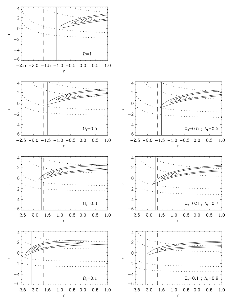
Figure 3: Constraints on the slope of the power spectrum ($n$) and the entropy evolution parameter ($\epsilon$) for seven different cosmological scenarios. Solid contours are the $68\%$ and $95\%$ confidence regions from the evolution of the X–ray luminosity function, using the combined data from all of the surveys. Dotted contours represent the $68\%$ and $95\%$ confidence regions for evolution of the cluster luminosity–temperature relation. Shaded regions are for parameters consistent with the evolution within $68\%$ limits (of both XLF and $L_{\rm x}-T$). The vertical solid line is the determination of $n$ from the CDM based theoretical calculation in Section 3.4 and the vertical dashed line is a measured value of $n$ from the APM rich cluster sample.

For each of the fiducial values of $\Omega_{0}$ (in both open and flat Universes), we determined the likelihood distribution as a function of $n$ and $\epsilon$. Initially, we analysed the data–sets independently, however the results show similar trends, albeit less constrained than the overall likelihood distribution, generated from combining all of the XLF data. We therefore focus our discussion using the combined XLF data–set – the result of this is shown in Figure 3. Clearly, this illustrates how the constrained area of parameter space changes with the background cosmology. This is the result of an interplay between two contributing factors, namely the model scaling relations used to fit the high redshift data and the positions of the data–points themselves, relative to the local XLF and $L_{\rm x}-T$ relation.

Constraints from the evolution of the $L_{\rm x}-T$ normalisation show a weak degeneracy between $n$ and $\epsilon$ for high values of $\Omega_{0}$. As $\Omega_{0}\rightarrow 0$, the range of $\epsilon$ becomes independent of $n$ (centred on $\epsilon=0$). The range of $n$ is unconstrained for all values of $\Omega_{0}$. The reason for the degeneracy is straightforward. The data imply no net evolution of the $L_{\rm x}-T$ normalisation for an empty Universe ($\Omega_{0}=0$). Hence, increasing the value of $\Omega_{0}$ pushes the high redshift sample to lower luminosities, prompting positive evolution in temperature for a fixed value of $L_{\rm x}$. In an $\Omega=1$ Universe with no entropy evolution ($\epsilon=0$) and a power spectrum with a negative slope, the model over–predicts the cluster luminosities, hence positive entropy evolution is required to match the data. As $n$ increases, the over–prediction becomes less severe (hence $\epsilon$ decreases). For $\Omega_{0}<1$ cosmologies, the amount of evolution required becomes progressively weaker as $\Omega_{0}$ decreases. Since the growth of structure is also slower, the data becomes more and more consistent with $\epsilon=0$ for all values of $n$.

The results from constraining the evolution of the combined XLF data–sets show a degeneracy in the opposite sense: higher values of $n$ demand higher values of $\epsilon$. This relation can be clearly explained from the $\Omega=1$ plot alone. Again, the model scales the XLF in such a way that for $\epsilon=0$, the result is an over–prediction of the cluster luminosities. However, this effect becomes less pronounced as $n$ decreases, leading to lower values of $\epsilon$. Eventually, the local luminosity function is shifted so much that the curvature becomes important, leading to an under–prediction of the abundance of clusters at the faint–end, where most of the data–points lie. This effect places a lower limit on the value of $n$. For lower values of $\Omega_{0}$, the data–points are pushed to brighter luminosities, as well as lower values of $dn/dL_{\rm x}$. Although the faint–end data are consistent with no evolution for $\Omega=1$, the re–scaling forces the points below the local XLF for lower values of $\Omega_{0}$. The brighter data (in particular the EMSS 2 point) is less sensitive to the change in cosmology, due to the steeper slope of the XLF. Coupled with the fact that the evolution of structure is weaker, an adequate fit to the data is allowed for more negative $n$.

In comparison to the open models, the flat ($\Omega_{0}+\Lambda_{0}=1$) models show slight variations in the constrained region of parameter space. The reason for the difference is two–fold. Firstly, the data–points themselves are scaled differently between cosmologies than their open counterparts. This is because the distance to a fixed redshift is larger for flat models (hence also increasing the volume element). This has the effect akin to having an open model with a lower value of $\Omega_{0}$. Secondly, the growth of structure in a flat model is more rapid than the corresponding open case, which affects the model scaling relations not unlike an open model with a higher effective $\Omega_{0}$.

Combining the constraints from the $L_{\rm x}-T$ and XLF measurements, we are unable to determine the value of $\Omega_{0}$ (with or without $\Lambda_{0}$) from the data alone: there is always a region of parameter space consistent with both observations. The same conclusion applies to all of the individual XLF data–sets. Specifically, the faint–end data–points from the ROSAT surveys are unable to set tight constraints; however they are able to set a lower limit on the slope of the power spectrum that is sensitive to the value of $\Omega_{0}$. The EMSS samples, particularly the EMSS 2 cumulative point, start to provide tighter limits on $n$ and $\epsilon$, since these results have started to probe the more sensitive luminosity range, brighter than $L_{\rm x}^{*}$. Therefore, future surveys will be more efficient at extracting information on the evolution of clusters by covering larger areas of sky, probing luminosities around and beyond $L_{\rm x}^{*}$.

3.4 Breaking the n–$\Omega_{0}$ degeneracy

It is evident that the model is unable to determine a value of $\Omega_{0}$ from the XLF and $L_{\rm x}-T$ normalisation constraints alone – a feasible range of $n$ and $\epsilon$ can always be found for the particular scenario. Noting that the constrained range of $n$ is sensitive to $\Omega_{0}$, combining an independent determination of $n$ with the X-ray data will be able to place a significant constraint on the value of $\Omega_{0}$. There are two ways in which this can be achieved: a theoretical prediction of the primordial power spectrum that gives the (cosmology–dependent) slope on cluster scales or a direct measurement from redshift surveys.

For the theoretical case, we need to obtain the local slope of the power spectrum on cluster scales, $n_{\rm eff}$ such that

$$n_{\rm eff}=\left.{d{\rm ln}P\over d{\rm ln}k}\right|_{k_{\rm eff}}.$$ (3.17)

Although there has been feverous debate recently, the currently most popular cosmogony is that dominated by cold dark matter (CDM), with $n\rightarrow 1$ for small $k$, turning over to $n\sim-3$ on small scales. We have adopted the transfer function given by Bardeen et al. ([1986]). The turnover scale is determined by the shape parameter, $\Gamma$, which is in turn, determined by the cosmological model:

$$\Gamma=\Omega_{0}\mbox{h}\,\exp\left[-\frac{\Omega_{b}}{\Omega_{0}}\,\left(\Omega_{0}+\sqrt{2\mbox{h}}\right)\right].$$ (3.18)

([1995]). We take the value $\Omega_{b}=0.013\,\mbox{h}^{-2}$ from nucleosynthesis constraints ([1995]). No contribution enters from the cosmological constant, due to the fact that it contributed negligibly to the energy density at the last scattering epoch. To estimate $k_{\rm eff}$, we assume that the virial mass of a typical rich cluster in the local Universe (e.g.  the Coma cluster) is $M\sim 5\times 10^{14}\,\hbox{h}^{-1}\,\hbox{M}_{\odot}$. If the cluster formed by the top–hat collapse of a spherically overdense region, the comoving radius required to contain this mass (assuming present background density) would be $R\sim 8\,\hbox{h}^{-1}\,\hbox{Mpc}$ ([1996]). This is only true for a critical density Universe but can easily be modified for lower densities, since $R\propto\Omega_{0}^{-\frac{1}{3}}$. The value of $R$ can then be converted to an effective scale on the linear power spectrum by using the following formula ([1994]):

$$k_{R}=\left[{\left[\frac{1}{2}(n+1)\right]!\,\over 2}\right]^{1\over n+3}\,{\sqrt{5}\over R},$$ (3.19)

which should iteratively converge on the values $(n_{\rm eff},k_{\rm eff})$, with the use of equation 3.17. The calculated values of $n$ are represented as solid lines in Figure 3. Note that the value of $n$ becomes more negative with decreasing values of $\Omega_{0}$. Although the effective scale of galaxy clusters is larger in a low mass–density Universe, the change in shape of the CDM power spectrum itself (parametrised by $\Gamma$) dominates the shift in the value of $n$. As $\Omega_{0}$ decreases, the position of the turnover moves to larger scales, leading to a more negative slope on cluster scales. Figure 3 shows the result of this calculation, plotted as a solid vertical line. Analysing the likelihood distributions for a continuous range of $\Omega_{0}$, we find that the CDM prediction is only consistent with the X–ray data for $\Omega_{0}<0.55$ ($\Lambda_{0}=0$) and $0.1<\Omega_{0}<0.7$ ($\Omega_{0}+\Lambda_{0}=1$), to $95\%$ confidence. We can place a lower limit on $\Omega_{0}$ in the flat model because the predicted value moves to more negative $n$ faster than the XLF contours, as $\Omega_{0}$ decreases.

Another approach is to constrain $n$ directly by measuring the power spectrum on rich cluster scales from wide–area sky surveys. One example ([1997]) comes from the APM cluster sample, which has a median redshift $\left<z\right>=0.09$, measuring a slope, $n_{\rm APM}=-1.6\pm 0.3$. We currently assume that the underlying power spectrum has negligible curvature on the range of scales we are studying. Ideally, we would separate the population into redshift bins and scale each respective population relative to the preceeding one, using the slope of the spectrum at that epoch. Imminent surveys such as the Sloan Digital Sky Survey and the 2dF Galaxy Redshift Survey should provide the necessary data to constrain the slope at higher redshifts. Furthermore, the APM result assumes that the bias is linear and therefore scale–invariant on scales of the mean inter–cluster separation.

Survey	$\Omega_{0,u}(\Lambda_{0}=0)$		$\Omega_{0,u}(\Lambda_{0}=1-\Omega_{0})$
SHARC	$1.0$	$[0.6,>1.0]$	$1.0$	$[0.5,>1.0]$
WARPS	$1.0$	$[0.75,>1.0]$	$1.0$	$[0.7,>1.0]$
RDCS	$1.0$	$[0.65,>1.0]$	$1.0$	$[0.6,>1.0]$
EMSS 1	$1.0$	$[0.7,>1.0]$	$1.0$	$[0.6,>1.0]$
EMSS 2	$0.7$	$[0.4,>1.0]$	$0.65$	$[0.3,>1.0]$
COMBINED DATA	$0.4$	$[0.25,0.6]$	$0.4$	$[0.2,0.65]$

Table 3: Upper limits on the value of $\Omega_{0}$ (with and without $\Lambda_{0}$), using the constraint that $n=-1.6$, from the APM survey (Tadros, Efstathiou & Dalton, 1997). Results from both individual and combined XLF data–sets are presented. Limits are set using the $95\%$ confidence limits consistent with both the XLF and $L_{\rm x}-T$ constraints. Ranges in square brackets are for quoted uncertainties in $n$ ($\pm 0.3$)

To constrain the range of $\Omega_{0}$, we took the $95\%$ limits placed on $n$ and $\epsilon$ from the evolution of the XLF and $L_{\rm x}-T$ normalisation and subsequently fixed the value of $n$ to $-1.6$. For the XLF data, we found that the model fits the data more and more adequately as $\Omega_{0}$ decreases (for the range of $n$ considered): this is shown in the plot by the shift in the contours. Hence, this prevents us from placing a lower limit on $\Omega_{0}$. In the flat models the geometry weakly alters the shape of the likelihood distribution but the overall trend is the same. Since both constraints produce contours that become more aligned in lower $\Omega_{0}$ cosmologies, we are unable to make further conclusions regarding the lower limit.

What the data does allow us to do is place an upper limit on the value of $\Omega_{0}$. The results are given in Table 3, displaying the values that are consistent with the $95\%$ confidence limits of the XLF and $L_{\rm x}-T$ relations. Results for both the individual and combined XLF data–sets are presented. The ranges in brackets were determined by varying the value of $n$ by $\pm 0.3$. It is evident that the value of $\Omega_{0}$ is unconstrained using the APM value, for all of the individual data-sets except the EMSS 2 survey. The flat models give similar results to their open counterparts, with the range in the upper limits being slightly larger. Combining the XLF surveys sets a tighter constraint: $\Omega_{0}<0.6$ (or equivalently $\Omega_{0}<0.65$ for $\Omega_{0}+\Lambda_{0}=1$).

3.5 Evolution of Cluster Core Sizes

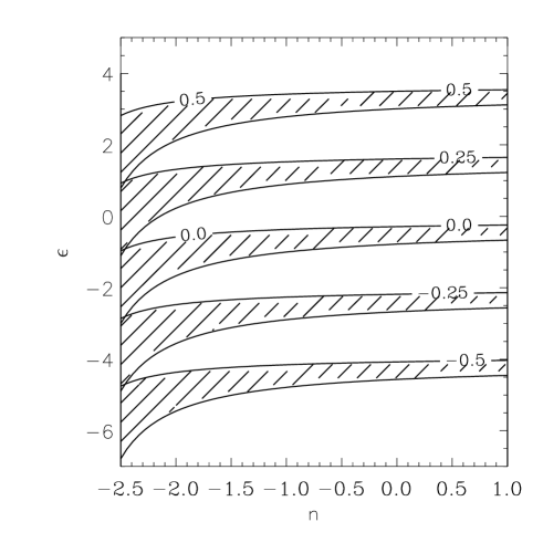
Figure 4: The region of parameter space covered by evolution of the cluster core radius for various models. The shaded regions depict the range of cosmologies, from $\Omega=1$ (with the greatest amount of structure evolution) to $\Omega=0.1,\Lambda_{0}=0.0$ (with the least amount of structure evolution). Each particular area illustrates the different amount of evolution in the redshift range $z=[0.0,0.5]$, with the labels indicating the value $\Delta{\rm log}r_{c}.$

Finally, we consider another possible constraint that could be readily measured from X–ray data: the evolution of cluster core–radii. Using the model we developed in section 2.3, we predict the characteristic core-radius of a cluster population to scale as:

$$r_{c} \propto \delta_{+}^{a}\,(1+z)^{b}\,(1+z_{f})^{c}\,\left({\Delta_{vir}\over\Omega}\right)^{d},$$ (3.20)

$$a = {2\over n+3}\left(1-\frac{1}{\beta}\right),$$

$$b = {\epsilon\over 2\beta},$$

$$c = {1\over 2\beta}-1,$$

$$d = \frac{1}{3}\left({1\over 2\beta}-1\right).$$

Even though the core radius depends on both $n$ and $\epsilon$, it’s evolution is determined much more sensitively by the changes in the central entropy of the gas rather than the amount of structural evolution. Figure 4 illustrates the regions of parameter space consistent with various amounts of core radius evolution, out to a redshift $z=0.5$. The background cosmology and spectral index have only a weak influence on the evolution of $r_{c}$, hence observations should quite easily place a constraint on the value of $\epsilon$ – the two extremes of the shaded regions represent scaling in the core by a factor of $\sim 0.3$ and $3$ respectively. Core sizes that shrink with redshift demand negative values of $\epsilon$ (i.e.  the core entropy of clusters decreases with redshift) whereas core sizes that grow with redshift demand values of $\epsilon$ that are weakly negative or higher. This approach is useful in the sense that we can directly measure the rate of entropy evolution in the core and test it’s consistency with the other methods presented above.

Analysis involving looking at changes in the cluster core size has now started to appear in the literature. Results are currently suggesting no significant evolution in the core size, at least out to $z\sim 0.5$ ([1998]). Given the uncertainties, our results are consistent with this, however positive evolution in the cluster core radii ($\epsilon>0$) would be preferred. At present, the sample sizes are small: a more comprehensive measurement of core radius evolution will serve as an important test of the validity of this model.

4 Discussion

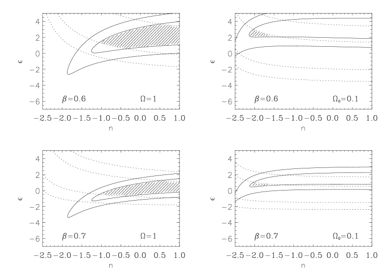
Figure 5: An example of the effect of varying $\beta$ using the SHARC XLF data. The left column is for $\Omega=1$ (the most mass evolution) and the right column $\Omega_{0}=0.1$ (the least mass evolution). The top and bottom rows for the expected limits on $\beta$ (0.6 and 0.7 respectively). The effect on $n$ is insignificant, although raising $\beta$ lowers the range of $\epsilon$.

At this stage, we go on to focus on several issues that are worthy points for discussion. Firstly, our results are based on several important assumptions made when modelling the X–ray evolution of clusters, so we discuss our choices and their robustness. Secondly, particularly due to the recent publication of ROSAT and ASCA data, several results constraining $\Omega_{0}$ using the evolution of X–ray clusters have now appeared in the literature. We therefore compare our results with those found by other groups. Finally, we address what we think is an important strategy for observations (particularly with the imminent launch of the XMM satellite, and pin–point the areas that we think will maximise future success in this field.

4.1 Model Assumptions

Although general and based on physically motivated scaling relations, there are several key approximations in the model used to arrive at this conclusion. One example is the $\beta$ profile: the results presented in §3 assume that the X–ray emission profiles are well fit when using the $\beta-\hbox{model}$, where the density of the intracluster gas tends to a constant value at small r (the core) and the isothermal result at large r, for a value of $2/3$. Individual measurements of $\beta$ do not necessarily give this value, although we assume that the average value over the population at a given epoch is well represented by $\left<\beta\right>=2/3$. However, it is important to investigate the tolerance of the model when varying the value of $\beta$. Figure 5 illustrates the effect on the constrained range of $n$ and $\epsilon$ that variations in $\beta$ induces. Using the SHARC data as an example, we have taken two values of $\beta:0.6$ and $0.7$, defining what we think are the expected limits of any fluctuation. Two cosmological models have been chosen : $\Omega=1$ and $\Omega_{0}=0.1$, which represent the most and least amount of structural evolution respectively. Changing $\beta$ can significantly change the range of $\epsilon$ values but has relatively little effect on the values of $n$. This, coupled with the work on the core radius discussed in the last section, reinforces the idea that both $n$ and $\epsilon$ contribute separately to the evolution of clusters: the entropy evolution is sensitive to the way in which the gas is distributed, with $\beta$ and $r_{c}$ defining the shape of the gas density profile, while the mass evolution is tied in with the background density. Hence, the dependence of $\Omega_{0}$ on $\beta$ is weak, although certain models may be ruled out on the basis that the range of $\epsilon$ may be implausible. This is evident in the figure, where the combination $(\beta=0.6,\Omega_{0}=0.1)$ pushes allowed values of $\epsilon$ into the limit set by the maximum cooling calculation ($\epsilon=2.0$) given in Paper I.

With the Launch of the AXAF satellite, it will become possible to study the emission profiles of distant clusters in more detail. These studies may show that the cluster profile evolves with redshift. For example, simulations of cluster evolution with pre–heated gas by Mohr & Evrard ([1997]) suggest that the entropy injected reduces the overall slope of the gas density profile rather than just that of the profile of the very centre. This effect can be parameterised by a much slower role over near the core radius but the scaling of the solution remains the same, since the X–ray emission still scales as $\rho_{c}^{2}r_{c}^{3}T^{\alpha}$. Thus, as Figure 5 shows, the $\beta$ profile and the $\epsilon$ parameter are interconnected – while observations of the emission profiles of high redshift clusters would cause us to revise our physical interpretation of a particular $\epsilon$ value, and re–examine the balance of heating and cooling within the cluster, it would not invalidate the phenomenological description provided by the model.

We may apply the same argument to take into account the non–isothermal temperature of structure of clusters suggested by [1998]. The model only requires that the temperature structure is normalised by the virial temperature of the dark matter halo. The temperature structure may affect the rate at which the cluster core evolves for a given entropy change, but this should again taken into account when the $\epsilon$ parameter is interpreted.

The model has been developed under the assumption that clusters of galaxies are in dynamical equilibrium. Clusters that are seen during major mergers may have X–ray luminosities and average temperatures that are far from their hydrostatic values. Nevertheless, the description we have developed applies to the cluster population as a whole, and the properties of individual clusters may differ wildly from the average. In this sense, the effects of mergers are already incorporated through the entropy evolution described by the model, and the disruption of hydrostatic equilibrium is mimicked by an increase in core entropy. The cluster temperatures are also susceptible to these departures, however, since they are weighted by the luminosity. Ideally, we should use cluster temperatures measured from the outer regions of clusters where the gas temperature better reflects the virial temperature of the gravitational potential. These are not available for distant clusters at present, but our results will still be valid so long as the evolution of the luminosity weighted temperature reflects the evolution of the cluster potential. This is a problem common to all methods based on the X–ray temperatures of clusters.

The slope of the luminosity–temperature relation does not explicitly enter our determination for the evolution of clusters. All that is required in our model is the evolution of the normalisation. We have implicitly assumed that the slope remains fixed at its present–day value. This assertion, which corresponds to the assumption that the entropy evolution parameter ($\epsilon$) is independent of cluster temperature, is unavoidable with the limited temperature data that is available for high redshift clusters. Consequently, it is important that the evolution of the normalisation is determined by using consistent slopes for high and low redshift data, and preferably using high redshift clusters representative of the clusters used to determine the luminosity function evolution. At present, temperature measurements are available only for the brightest clusters at high redshift. This situation will hopefully improve with the launch of the XMM satellite ([1996]); its large collecting area is ideally matched to the determination of temperatures for the lower luminosity, distant clusters. The slope of nearby ($z<0.05$) clusters has been most recently determined by Markevitch ([1998]), using ROSAT luminosities and ASCA temperatures, measuring a value, $\lambda\sim 2.65$. However, we make use of the older sample based on Einstein MPC data ([1993]) for two reasons. Firstly, constraints on the evolution of the $L_{\rm x}-T$ relation are provided by Mushotzky & Scharf ([1997]), which uses this (local) sample to contrast with their higher redshift ($\left<z\right>\sim 0.3$) ASCA data. Also, the slope supplied by Markevitch has been calculated for clusters with cooling flows removed, in order to directly compare with models that exclude non–radiative components in the plasma evolution. Since our model is based on evolution of the central entropy, we cannot exclude the cooling flow clusters, which probably contribute to most, if not all of the negative entropy evolution in cluster populations. We argue that the dominant cause for the intrinsic scatter in the relation is due to each cluster having it’s own particular core entropy, coming from their individual formation histories.

The considerations we discussed above related to the distribution of gas within the dark matter potential. In a low density universe, it is necessary to explicitly account for the distinction between the background density of the Universe when the cluster is formed, and it’s value when the cluster is observed. We have related these two epochs by assuming that the mass of the cluster grows by a factor of two (Kitayama & Suto, 1996). However, for $\Omega_{0}>0.1$, this factor produces only a small change in the halo evolution.

4.2 Comparison with Other Methods

A number of other papers have recently appeared in the literature dealing with the constraints on $\Omega_{0}$ from the X–ray evolution of clusters. One of the most popular methods uses the evolution of the cluster abundances (e.g.  [1997], [1998], [1998], [1998], [1997], [1998]). To extract the value of $\Omega_{0}$, an estimator for the cluster virial mass is required. This can be achieved by calculating the cluster temperature function at any given epoch and converting this to mass using the Press–Schechter formalism with the assumption that the cluster haloes form via spherical infall. The result from this method is still slightly unclear – at present the majority of authors find values of $\Omega_{0}$ typically in the region $0.3-0.5$ with or without $\Lambda$, although some authors find higher values including $\Omega=1$ (e.g.  [1998], [1998]). An extensive discussion on the existence of this clash in results can be found in Eke et al. ([1998]). In particular, they highlight the discrepancy in the abundance of low–redshift clusters, particularly the high temperature end, where the measured value is uncertain. Those favouring high $\Omega_{0}$ assume a higher abundance of clusters in this region than those favouring low values of $\Omega_{0}$.

Our work differs from these treatments in that it does not assume a detailed model for the abundance of clusters or for their temperature or X–ray luminosity distribution. Instead, we have emphasised the scaling relations that must relate the properties of clusters at one epoch with those at another. By introducing an additional parameter that describes the evolution of the core gas entropy, our approach allows us to inter–compare clusters at different epochs with minimal further assumptions. Comparing our results with those obtained by other authors illuminates the constraints which are general and those which are model–specific. As an example, Reichart et al. ([1998]) also look at luminosity function evolution by adopting the Press–Schechter approach for the evolution of the mass function , but use the $L_{\rm x}-T$ relation to calibrate their mass to X–ray luminosity relation. In addition, their model differs from ours in that it involves the slope of the $L_{\rm x}-T$ relation explicitly, resulting in a purely empirical calibration of the luminosity–mass conversion. By contrast, our approach uses the weak self–similarity principle (plus the entropy evolution) to scale the properties of clusters between epochs. As discussed extensively in Paper I, this is completely separate from the scaling relations between clusters of different mass at the same epoch. Trying to equate the two requires that we adopt a Strong Self–Similarity principle; something for which there is little physical justification. Reichart et al. adopt the same parameterization as Evrard & Henry ([1991]), notably $L_{\rm x}\propto T^{p}(1+z)^{s}$; assuming $\beta=2/3$, we find for our model that $p=13/6$ and $s=(13-3\epsilon)/4$. However, as we have emphasised, the way in which we constrain our parameters (particularly $\epsilon$ in this context) is fundamentally different, and we should not expect to obtain identical results.

We choose to concentrate our comparison with the work of Eke et al. ([1998]). These authors derive a value of $\Omega_{0}$ from the evolution of the cluster temperature function, using emission–weighted temperatures obtained from ASCA data ([1997]). Since the cluster sample is X–ray flux limited, they have to correct for incompleteness in their estimation of the temperature function. This is done by assuming a non–evolving $L_{\rm x}-T$ relation (i.e.  fixed slope, normalisation and scatter). The advantage of this method is that it infers the mass distribution in a more direct manner than our approach, hence their work places a strong constraint on $\Omega_{0}$: $\Omega_{0}=0.43\pm 0.25$ for $\Lambda_{0}=0$ and $\Omega_{0}=0.36\pm 0.25$ with a non–zero cosmological constant. This was achieved with a substantially smaller data–set. Furthermore, the authors were able to internally constrain the shape of the power spectrum. This is possible because they directly link the form of the temperature function to the mass function through the Press–Schechter model (assuming a CDM power spectrum). They arrive at a value of $\Gamma$ of $0.08\pm 0.07$ ($\Gamma=0.09\pm 0.08$ for $\Omega_{0}+\Lambda_{0}=1$).

To compare our results to those of Eke et al., we first convert their measured range of $\Gamma$ to an equivalent range of $n$, using the same method discussed in section 3.4. We then find the range of $\Omega_{0}$ that is both consistent with the X–ray data and the calculated range of $n$. We find that $\Omega_{0}<0.45(\Omega_{0}<0.5$ for $\Omega_{0}+\Lambda_{0}=1$) to $95\%$ confidence, in agreement with their upper limit. However, we fail to place a constraint on the lower limit of $\Omega_{0}$. This is initially surprising, but seems to be due to systematic differences in the data. We find that, for a low $\Omega_{0}$ cosmology, the available data are consistent with weak negative evolution of the XLF and no evolution in the $L-T$ normalisation. By contrast, Eke et al.’s temperature function data (corrected for cosmology) shows a decline in temperature function amplitude suggesting that a very low value of $\Omega_{0}$ is unacceptable due to the deficit of clusters at this epoch. Such dependence on the particular data set is worrying, but emphasises the importance of using independent data–sets to establish consistent conclusions and reduce systematic biases. It is satisfying to find that our method finds similar results, at least in determining the upper limit.

4.3 Future Directions

Since the results presented in this paper were based on scaling the ROSAT BCS XLF to fit the higher redshift surveys, we have assumed that the two populations are well separated in redshift. This is not immediately obvious, since the ROSAT BCS sample has clusters out to $z\sim 0.3$, where the other samples start around this value. The saving grace is that the higher–redshift surveys have detected lower luminosity clusters ($L_{\rm x}<L_{\rm x}^{*}$), due to the small solid angles of the surveys, whereas the BCS clusters in this regime are at much lower redshifts. However, this range of luminosities places a much weaker constraint on the model than if high redshift data were available at the brighter end ($L_{\rm x}>L_{\rm x}^{*}$). Improved coverage will result in a better internal constraint, since the effects of evolving cluster number density and cluster luminosity will be more easily separated. As a pointer for the future, what is required is a more statistically sound description of the high–redshift XLF from $L_{\rm x}^{*}$ and above. As an hypothetical example, we assume that the combined data–set used in this paper is a good description of the XLF for luminosities around and below $L_{\rm x}^{*}$. A measurement is then made at $L_{\rm x}(0.5-2.0\,\hbox{keV})\sim 10^{45}\,\hbox{erg}\,\hbox{s}^{-1}$, detecting 10 clusters at $\left<z\right>=0.5$ in a solid angle that resulted in a cumulative abundance in agreement with the BCS cumulative XLF ($N(>L_{\rm x})\sim 0.25\times 10^{-8}\,\hbox{Mpc}^{-3}$). This strongly suggests a detection of no evolution, particularly for the $\Omega=1$ geometry. Using the APM constraint on $n$, we find that $\Omega_{0}<0.2$ at the $99\%$ level. In practice, the XMM satellite is particularly suited to this task, with its large collecting area and high spatial resolution, that will allow one to easily make the distinction between clusters and AGN. What is required, however, is a wide area survey covering at least 500 square degrees, rather than a survey that is particularly deep. In the near term, progress will be made through the ROSAT North Ecliptic Pole survey – a wide angle survey composed of superposed ROSAT All–Sky Survey strips ([1999]).

5 Conclusions

In this paper, we have taken the entropy–driven model of cluster evolution, detailed in Bower (1997) for an $\Omega=1$ Universe, and modified it to account for evolution in different cosmological scenarios, specifically open models and flat, non–zero $\Lambda$ models. This allows us to separate contributions made by the hierarchical growth of structure (controlled by the slope of the power spectrum, $n$) and changes in the core entropy of the intracluster gas (controlled by the entropy evolution parameter, $\epsilon$).

We then placed constraints on $n$ and $\epsilon$ for seven reasonable cosmological models, using the current wave of X–ray data for the two observables: the X–ray Luminosity Function and the Luminosity–Temperature relation. For the $L_{\rm x}-T$ relation, we have taken the compiled low and high redshift samples from David et al. (1993) and Mushotzky & Scharf (1997) respectively and determined the best–fit slope and scatter. We subsequently placed 68% and 95% confidence limits on the evolution of the temperature normalisation, which is slope–dependent. For the XLF, we have used the recently available ROSAT samples, specifically the SHARC ([1997]), WARPS ([1998]) and RDCS ([1998]) high–redshift, non–parametric determinations, as well as the older EMSS samples ([1992], [1995]). The amount of evolution in these measurements was quantified by comparing with the local ROSAT BCS XLF ([1997]). Using the X–ray data alone, we find acceptable regions of parameter space for every cosmological model considered, to a high degree of confidence. Specifically, as the density parameter decreases, more negative values of $n$ are allowed to compensate for the weakening growth rate of clusters. Values of constrained $\epsilon$ are appropriate to modify the luminosity evolution to compensate for the measured change in abundance, moving weakly from positive values to zero (no evolution) for low–density Universes.

To break the degeneracy between $n$ and $\Omega_{0}$, we calculated the slope of the power spectrum based on the CDM paradigm, by taking the typical mass of a rich cluster and calculating the corresponding fluctuation scales that give rise to such objects. We find that the CDM calculation sets a limit of $\Omega_{0}<0.55$ ($0.1<\Omega_{0}<0.7$ for $\Omega_{0}+\Lambda_{0}=1$). Using the value determined by the APM survey ($n=-1.6\pm 0.3$), we conclude that $\Omega_{0}<0.6\ (<0.65$ for $\Omega_{0}+\Lambda_{0}=1$). All limits were calculated to $95\%$ confidence. In general, we cannot determine a lower limit to the value of $\Omega_{0}$, since our model fits the data much more comfortably at fixed $n$, for lower density Universes. The evolution of the cluster core–radius was also considered, where we showed that it depends much more sensitively on the entropy evolution of clusters than the structural evolution (determined by $n$ and $\Omega_{0}$). Present data suggest no strong evolution out to $z\sim 0.5$ ([1998]), roughly consistent with our results given the quoted uncertainties.

Finally, we discussed the robustness of assumptions we have made in the model, particularly the effect of varying the mass distribution of the gas (controlled by the value of $\beta$). Again, this has a much stronger effect on the constrained range of $\epsilon$ than the rate of structural evolution, and hence only weakly affects the determination of $\Omega_{0}$. We then compared our results to that of other groups, particularly with Eke et al. ([1998]). We find that our upper limit is consistent ($\Omega_{0}<0.45$, or $\Omega_{0}<0.5$ for $\Omega_{0}+\Lambda_{0}=1$ at $95\%$ confidence) although we cannot place a lower limit on $\Omega_{0}$.

In order to provide tighter limits on the value of $\Omega_{0}$, it will be essential to obtain an accurate measurement of the bright end of the XLF out to redshifts at least comparable to present distant cluster samples, ideally from a wide angle survey. This is something we hope that the forthcoming XMM mission can provide.

References

- [1986] Bardeen J.M., Bond J.R., Kaiser N., Szalay A.S., 1986, ApJ, 304, 15
- [1998] Blanchard A., Bartlett J.G., 1998, A&A, 332L, 49
- [1997] Bower R.G., Smail I., 1997, MNRAS, 290, 292
- [1997] Bower R.G., 1997, MNRAS, 288, 355
- [1996] Bower R.G. et al. 1996, MNRAS, 281, 59
- [1997] Burke D.J., Collins C.A., Sharples R.M., Romer A.K., Holden B.P., Nichol R.C., 1997, ApJ, 488, L83
- [1979] Cash W., 1979, ApJ, 228, 939
- [1997] Collins C.A., Burke D.J., Romer A.K., Sharples R.M., Nichol R.C., 1997, ApJ, 479, L117
- [1995] Copi C.J., Schramm D.N., Turner M.S., 1995, Science, 267, 192
- [1993] David L.P., Slyz A., Jones C., Forman W., Vrtilek S.D., 1993, ApJ, 412, 479
- [1997] De Grandi S., Molendi S., Bohringer H., Chincarini G., Voges W., 1997, ApJ, 486, 738
- [1996] Dekel A., Burstein D., White S.D.M., 1997, Critical Dialogues in Cosmology (Princeton 250th Anniversary) ed. N. Turok (World Scientific), p175 (astro-ph/9611108)
- [1997] Ebeling H., Edge A.C., Fabian A.C., Allen S.W., Crawford C.S., Boehringer H., 1997, ApJ, L479, 101
- [1998] Eke V.R., Cole S.M., Frenk C.S., Henry J.P., 1998, MNRAS, 298, 1145
- [1998] Eke V.R., Navarro J.F., Frenk C.S., 1998, ApJ, 503, 569
- [1996] Eke V.R., Cole S.M., Frenk C.S., 1996, MNRAS, 282, 263
- [1991] Evrard A.E., Henry J.P., 1991, ApJ, 383, 95
- [1994] Gioia I.M., Luppino G.A., 1994, ApJS94, 583
- [1998] Hasinger G., Burg R., Giacconi R., Schmidt M, Trumper J., Zamorani G., 1998, A&A, 329, 482
- [1999] Henry J.P. et al., 1999, in preparation
- [1997] Henry, J.P., 1997, ApJ, 489, L1
- [1992] Henry J.P., Gioia I.M., Maccacaro T., Morris S.L., Stocke J.T., Wolter A., 1992, ApJ, 386, 408
- [1984] Jones C., Forman W., 1984, ApJ, 276, 38
- [1998] Jones L.R., Scharf C., Perlman E., Ebeling H., Horner D., Wegner G., Malkan M., McHardy I., 1998, AN, 319, 87
- [1991] Kaiser N., 1991, ApJ, 383, 104
- [1997] Kitayama T., Suto Y., 1997, ApJ, 490, 557
- [1996] Kitayama T., Suto Y., 1996, ApJ, 469, 480
- [1991] Lahav O., Rees M.J., Lilje P.B., Primack J.R., 1991, MNRAS, 251, L128
- [1995] Luppino G.A., Gioia I.M., 1995, ApJ, 445, L77
- [1996] Lumb, D., Eggel, K., Laine, R., Peacock, A., 1996, SPIE, 2808, 326
- [1998] Markevitch M., 1998, ApJ, 504, 27
- [1998] Markevitch M., Forman W.R., Sarazin C.L., Vikhlinin A., 1998, ApJ, 503, 77
- [1998] Mathiesen B., Evrard A.E., 1998, MNRAS, 295, 769
- [1997] Mohr J.J., Evrard A.E., 1997, ApJ, 491, 38
- [1997] Mushotzky R.F., Scharf C.A., 1997, ApJ, L485, 65
- [1998] McHardy I.M. et al. 1998, AN, 319, 51
- [1997] Oukbir J., Blanchard A., 1997, A&A, 317, 10
- [1994] Peacock J.A., Dodds S.J., 1994, MNRAS, 267, 1020
- [1980] Peebles P.J.E., The Large-Scale Structure of the Universe, 1980, PUP, Princeton, NJ
- [1974] Press W.H., Schechter P., 1974, ApJ, 187, 425
- [1998] Reichart D.E., Nichol R.C., Castander F.J., Burke D.J., Romer A.K., Holden B.P., Collins C.A., Ulmer M.P., 1998, ApJ, submitted (astro-ph/9802153)
- [1998] Rosati P., Ceca R.D., Norman C., Giacconi R., 1998, ApJ, 492, L21
- [1998] Sadat R., Blanchard A., Oukbir J., 1998, A&A, 329, 21
- [1997] Scharf C.A., Jones L.R., Ebeling H., Perlman E., Malkan M., Wegner G., 1997, ApJ, 477, 79
- [1997] Smail I., Ellis R.S., Dressler A., Couch W.J., Oemler A., Butcher H., Sharples R.M., 1997, ApJ, 479, 70
- [1995] Sugiyama N., 1995, ApJS, 100, 281
- [1997] Tadros H., Efstathiou G., Dalton G., 1997, MNRAS, 296, 995
- [1996] Tsuru T., Koyama K., Hughes J.P., Arimoto N., Kii T., Hattori M., 1996, The 11th international colloquium on UV and X-ray spectroscopy of Astrophysical and Laboratory Plasmas
- [1998] Viana P.T.P., Liddle A.R., (astro-ph/9803244)
- [1998] Vikhlinin A., McNamara B.R., Forman W., Jones C., Quintana H., Hornstrup A., 1998, ApJ, 498, L21